Triple Filtering of Terrain Conductivity Data for Precise Tracing of Underground Utilities

Abstract

Terrain conductivity meters (TCMs) are efficient devices for different sorts of subsurface investigations, including detecting and tracing buried utilities, such as metallic pipes and cables. However, data collected using TCMs are usually ambiguous and hard to interpret. This ambiguity originates from the complex shape of apparent conductivity anomalies, the influence of irrelevant conductive bodies, and the interference of random noise with the collected data. To overcome this ambiguity and produce more interpretable apparent conductivity maps, a three-step filtering routine is proposed and tested using different real datasets. The filtering routine begins with applying a Savitzky–Golay (SG) filter to reduce the effect of random noise. This is followed by a modified rolling ball (MRB) filter to convert the complex M-shape of the anomaly into a single trough pointing to the underground utility. Finally, a virtual resolution enhancement (VRE) filter is applied to enhance the pinpointing apex of the trough. The application of the proposed filtering routine to apparent conductivity data collected using different terrain conductivity meters over different utilities in different urban environments shows a significant improvement of the data and an effective ability to reveal masked underground utilities. The proposed triple filtering routine can be a starting point for a new generation of TCMs with a built-in operation mode for instantaneous delineation and characterization of underground utilities in real time.

1. Introduction

Frequency-domain electromagnetic (FDEM) portable instruments, commonly called terrain conductivity meters (TCM), are popular geophysical investigation tools due to their versatility, noninvasiveness, and cost-effectiveness. Consequently, they are increasingly used in different fields, such as hydrogeology, environmental studies, archaeology, agriculture, exploration, engineering, and land management. One common application of TCMs is detecting and mapping different underground utilities [1,2,3,4,5,6]. Using TCMs in underground utilities investigations is encouraged for several reasons. These include the low price of the instruments, the ease and swiftness of field data acquisition, the capability to scan large survey areas at variable depths in a short time, and the simplicity of data processing and interpretation [7]. However, the data collected with TCMs are often hindered by different types of interference noise. This noise can be inherent to the method or induced by external factors, both of which create uncertainty and non-uniqueness in the collected data that obstruct their efficient use in precisely delineating and mapping subsurface utilities, especially in urban areas.

The first and most annoying issue with the data collected using TCMs is the complexity of the anomaly shape formed over the cylindrical shape of utilities. This anomaly is usually composed of a sharp negative trough surrounded by two asymmetrical positive peaks [6,7]. This complex anomaly shape becomes more problematic when anomalies arising from several utilities, buried next to each other, interfere and overlap. Installing underground utilities underneath or near the sidewalk is a common practice in urban areas.

The second issue is caused by the geometrical shape of the TCM and the way it is carried by the operator during field data acquisition. All TCMs have long booms that range from one meter to several meters and are carried on the shoulder of the operator using a wide belt. Accordingly, titling and swinging of the TCM while walking is inevitable, especially when data are collected in the continuous mode [7]. This horizontal and vertical swings of the two edges of the TCM change the geometrical relationship between the receiver and the transmitter coils with the subsurface object, which introduces short-wavelength noise into the collected data.

The third issue is the uneven background of the resultant terrain conductivity maps. This appears as a gradual change in background conductivity that is caused by either a change in soil nature when surveying large areas or by surface or subsurface utility mains, usually present on the edges of the surveyed areas. The same problem may arise from other surface sources of noise, such as reinforced concrete walls, street signs, parking vehicles, and other irrelevant surface objects typically found in urban areas. These three issues combined can obscure the targeted utility and make it difficult to pinpoint its exact location, causing digging and excavation to be large and messy [1].

This article introduces a simple and computationally light solution for these nagging noises, namely the triple filtering routine. This routine comprises three consecutive filters that transform the ambiguous and vague apparent conductivity maps into distinct maps, in which underground utilities induced anomalies are sharp, clear, and interpretable. This triple filtering produces clean apparent conductivity maps that precisely indicate and accurately delineate the subsurface utility under investigation. The triple filtering technique is tested using four sets of apparent conductivity data collected in urban areas in different cities inside the Kingdom of Saudi Arabia (KSA) using different TCMs and with different field data acquisition parameters.

2. Materials and Methods

The four datasets used to test the effectiveness of the triple filtering algorithm are selected from a group of surveys collected by the authors to investigate different types of utilities, using different TCMs, in different locations within the KSA. The reason for selecting such diverse datasets with variable field parameters for testing the proposed triple filtering process is to subject this new filtering technique to a real test and to check its capability to yield reasonably acceptable results irrespective of the data acquisition tool, the surrounding environment, and the targeted utilities.

All data were collected in urban areas in 4 cities of the Kingdom of Saudi Arabia (KSA). The first dataset is a part of a large survey conducted in Dammam City, at the eastern border of KSA, in an area covered with reclaimed soil that is composed mainly of marine sand mixed with quaternary deposits. The shallow subsurface layer in this area is composed of sand and silt with minute amounts of shale and clay [8].

The second dataset was collected in Jubail City, on the eastern border of KSA, within the old industrial complex. Most of the area at this site is covered by eolian sand dunes; however, the shallow soil layer in the surveyed area is composed mainly of a mixture of marine and non-marine partially compacted sand, silt, and clay [9].

The third test dataset is a portion of a survey conducted over some utilities in Mecca City, which lies within the western region of the KSA. The data were collected in an urban area where the shallow subsurface layer is mainly made up of alluvial deposits. These alluvial deposits are composed mainly of gravel, sand, silt, and clay in different proportions [10].

The fourth test dataset is part of a survey conducted in Jeddah City, the second-largest city in the KSA, with a population of about 5 million people. The city and surveyed area are located on the Red Sea Coast on the western borders of the KSA. The area is covered by alluvial sediments made of gravel, sand, silt, and clay [11].

2.1. Theoretical Background

Recent years have witnessed a significant growth in the use of TCMs in various engineering, environmental, archaeological, agricultural, and forensic fields [7]. TCMs can provide useful information about the shallow subsurface in a short time and at a relatively low cost, and they can map the subsurface in near real time. In addition, TCMs are stable, lightweight, easy to use, environmentally friendly, and can be operated by one person. However, data collected using different TCMs while studying utilities and infrastructures have some problematic distortions and interferences related to the complex shape of the anomalies, device tilting-induced noise, and gradual change in background apparent conductivity [5].

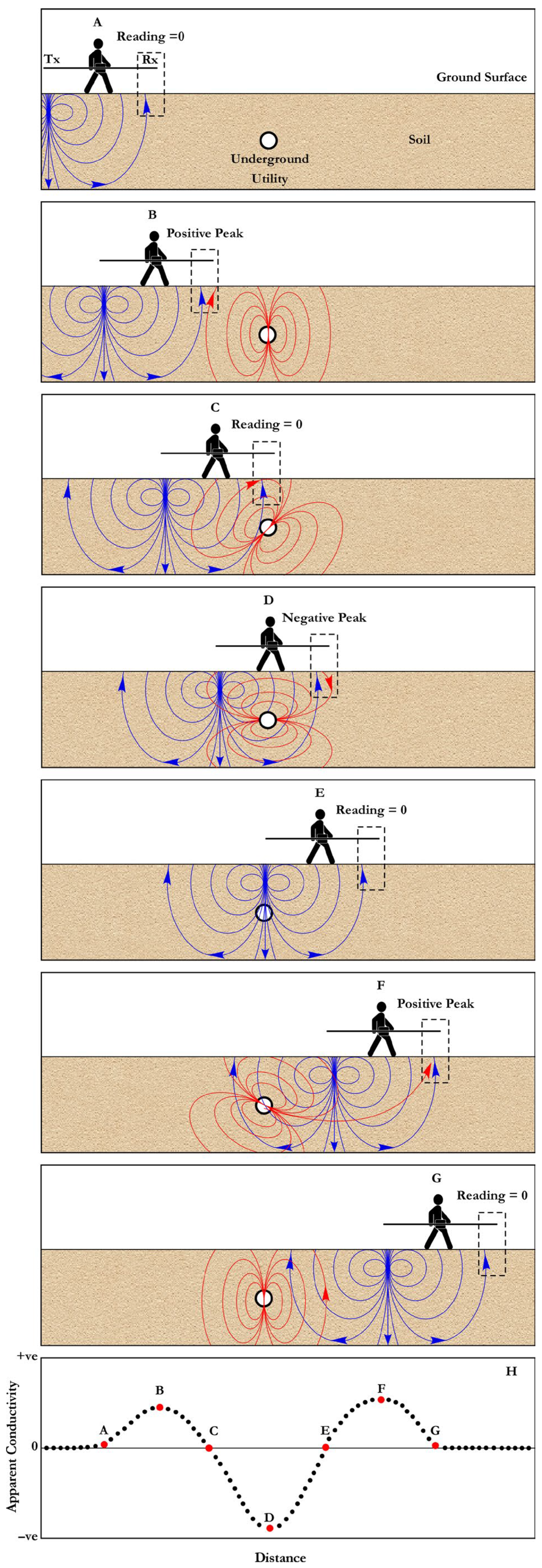
The problem of the complex anomaly shape is unavoidable and inherent in the principal working theory of these types of instruments that adopt the Slingram electromagnetic settings [12]. One common feature of all TCMs is that both the transmitter (Tx) and the receiver (Rx) are mounted inside the boom with a coil separation that ranges from less than a meter to several meters (Figure 1). While in operation, the transmitter, usually at the rear end of the boom, is energized with a time-harmonic current, which results in a primary electromagnetic field (blue lines in Figure 1). When this primary field encounters a metallic object, it creates an eddy current in that object, resulting in an induced secondary electromagnetic field (red lines in Figure 1). The resultant electromagnetic field is a combination of the primary and the secondary fields [12].

The resultant electromagnetic field, which is a combination of the primary and the secondary fields, is sensed by the receiver mounted at the front end of the boom. Because the primary field is compensated for via an inner connection between the transmitter and the receiver, only the secondary field is accounted for. The secondary field is decomposed by the TCM into in-phase and quadrature components [7]. When the spacing between the transmitter and the receiver is less than the skin depth, a low induction number condition is fulfilled. Under this condition, the subsurface apparent conductivity is directly proportional to the quadrature component of the secondary field and can be expressed by the following equation [13]:

$${\sigma }_a={\displaystyle \frac{4}{\omega {\mu }_0{S}^2}}{\left({\displaystyle \frac{H_S}{H_P}}\right)}_Q$$

(1)

where ${\sigma }_a$ is the apparent electric conductivity, ω is the angular frequency, μ₀ is the magnetic permeability of free space, S is the spacing between the transmitter and the receiver coils, and ${\left({\displaystyle \frac{H_S}{H_P}}\right)}_Q$ is the ratio between the quadrature components of the secondary and the primary fields at the receiver coil. This specific working principle of TCM is the main reason for the complex shape of TCM anomalies, as explained in Figure 1 [14].

When the surveyor is in position (A), the transmitter is too far from the subsurface object to induce any secondary field, and the TCM reads approximately zero (Figure 1A,H). As the surveyor moves to point (B), a secondary field is induced in the subsurface object. The directions of both the primary field and the secondary field coincide at the receiver vicinity. This alignment of the primary field and the secondary field perpendicular to the receiver coil plane causes TCM to read a positive value, resulting in a positive peak (Figure 1B,H). When the surveyor moves to point (C), the receiver becomes positioned above the subsurface object where the secondary field lines are running parallel to the ground surface and the receiver coil plane [13]. Consequently, no secondary field is sensed by the receiver, and the TCM reads zero (Figure 1C,H). At point (D), the induced secondary field lines have opposite directions to the primary field lines, and both the transmitter and the receiver are close to the subsurface object, which causes a sharp, strong negative trough (Figure 1D,H).

As the surveyor moves to point (E), the transmitter is exactly over the object and in the same plane as the object. This creates a situation where no secondary field is induced in the conductor, and only the primary field is sensed by the receiver coil, causing the TCM to read zero (Figure 1E,H). As the surveyor moves to point (F), the secondary field aligns with the primary field perpendicular to the coil plane, creating a positive peak [14]. This peak, however, is stronger than the positive peak at position (B) because the transmitter coil is closer to the subsurface metallic object in this case (Figure 1F,H).

When the surveyor moves to point (G), the transmitter coil is again too far from the object to induce any secondary field, and the TCM reads zero again (Figure 1G,H). This mechanism creates the unique bimodal asymmetrical M-shape anomaly for every subsurface metallic object (Figure 1H).

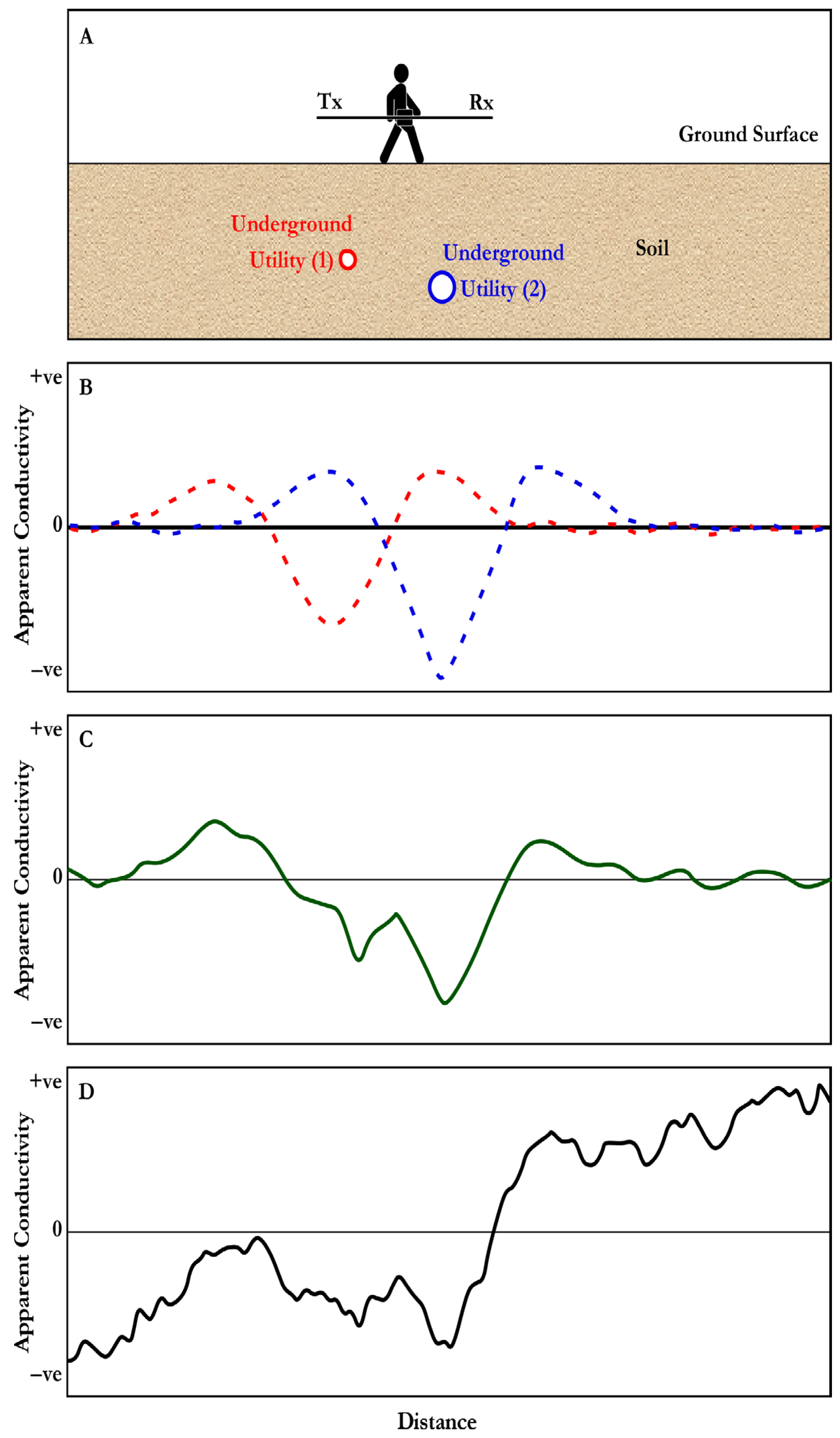
The issue of the complex shape of TCM anomalies becomes even more problematic when two or more anomalies superimpose and interfere with one another, creating a complicated anomaly shape that can be challenging to interpret. Figure 2A shows a situation where a surveyor encounters 2 neighboring underground utilities. Figure 2B shows the anomaly that arises from each anomaly, while Figure 2C shows the complex anomaly resulting from the summation of the 2 anomalies shown in Figure 2B. Such a complex anomaly is hard to disentangle and hence difficult to interpret [15].

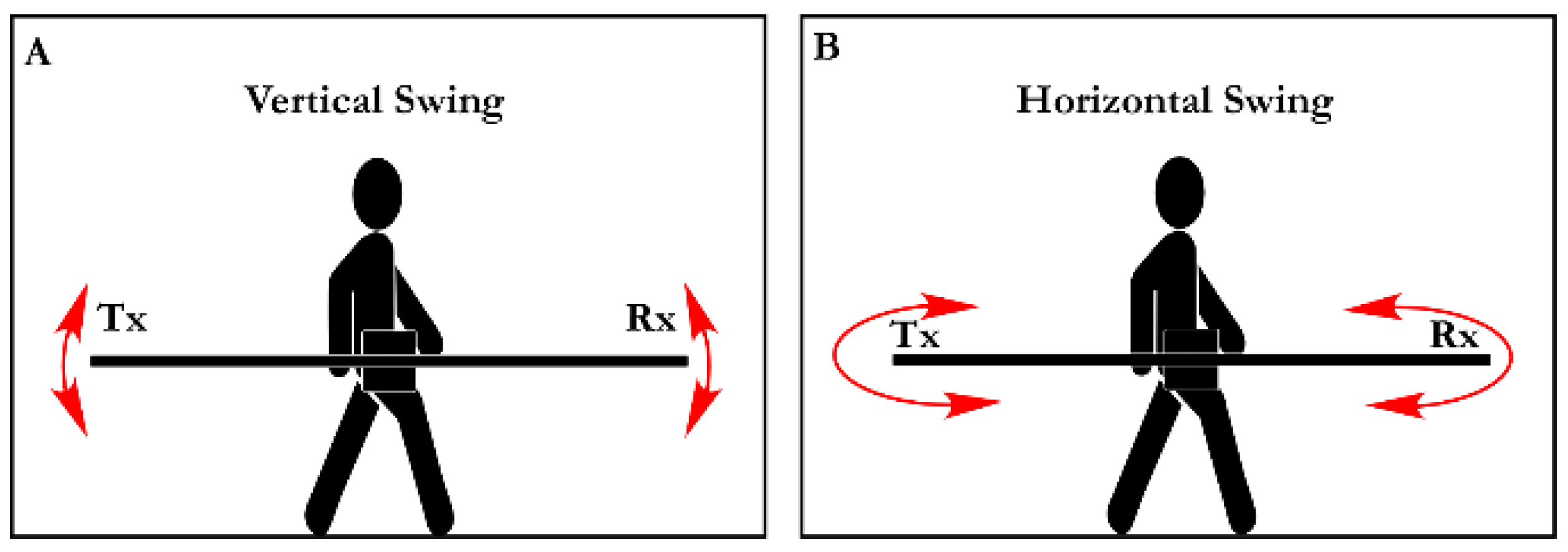
The second problem with TCM data is the random short-wavelength noise caused by the tilting and swinging of the boom of the carried meter while walking. This is most significant when the continuous data acquisition mode is used. As the surveyor carries the TCM and walks while holding the central part of the meter, the 2 ends of the TCM inevitably rotate along their vertical and horizontal planes (Figure 3).

These small movements are particularly noticeable when using relatively heavy TCMs with a long boom, such as the EM-31, where it is difficult to keep the boom straight and maintain smooth movement. This type of fluctuation causes small temporal variations in the geometrical relationships between the transmitter, the receiver, and the underground object, introducing random variations in the apparent conductivity data, as shown in Figure 2D. These variations degrade data quality and reduce the effectiveness of some processing tools, such as the rolling ball background removal [1].

When the surveyor moves to point (G), the transmitter coil is again too far from the object to induce any secondary field, and the TCM reads zero again (Figure 1G,H). This mechanism creates the unique bimodal asymmetrical M-shape anomaly for every subsurface metallic object (Figure 1H). This complex asymmetrical M-shape anomaly is inherent in the working mechanism of all TCMs adopting the Slingram electromagnetic setting and is unavoidable while crossing over a subsurface anomalous object [11,12,13,14,15]. Disentangling these complex and overlapping anomalies is essential for a precise interpretation [7].

These small movements are particularly noticeable when using relatively heavy TCMs with a long boom, such as the EM-31, where it is difficult to keep the boom straight and maintain smooth movement. This type of fluctuation causes small temporal variations in the geometrical relationships between the transmitter, the receiver, and the underground object, introducing random variations in the apparent conductivity data, as shown in Figure 2C. These variations degrade data quality and reduce the effectiveness of some processing tools, such as the rolling ball background removal [1].

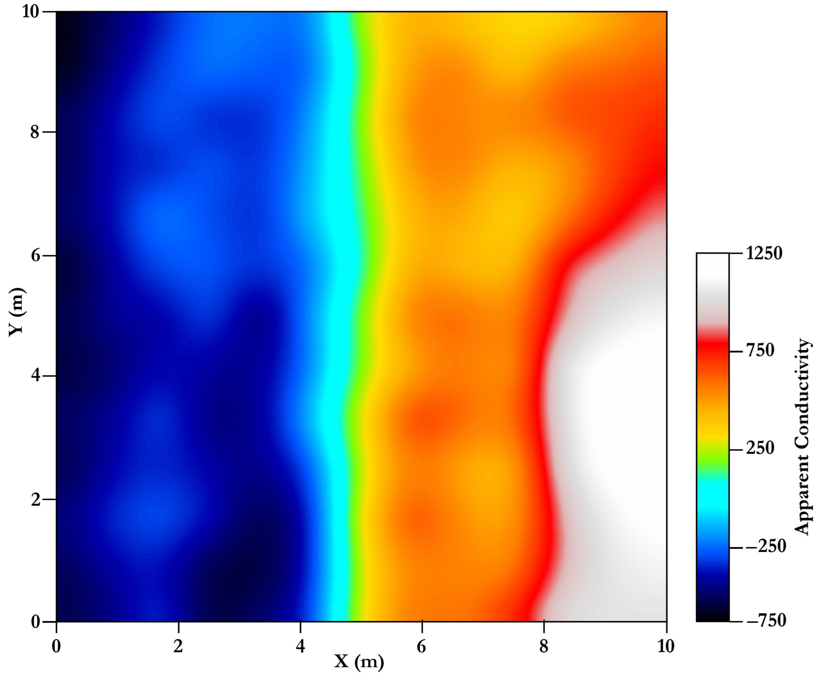
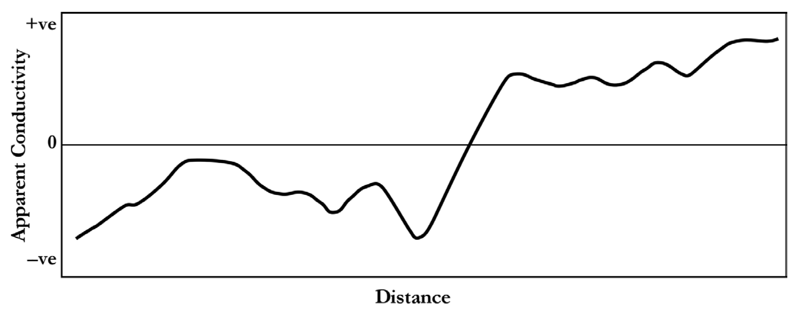
Finally, the third problem is the large noise bursts that come from irrelevant surrounding metallic bodies. While surveying urban areas, such noise sources are unavoidable and can produce high-amplitude noise that ruins the resultant apparent conductivity maps and may mask anomalies caused by objects of interest, such as underground utilities. One source of this nagging type of noise is related to the surface outlets, usually connected to the underground utilities. Examples of these are electrical kiosks connected to underground power cables, fire hydrant faucets connected to underground water pipes, and junction boxes connected to underground communication cables. These objects usually lie near the edge of the survey grid and produce remarkable changes in apparent conductivity readings. This results in unbalanced apparent conductivity maps, where the background on one side, or one corner, of the grid is relatively high and gradually decreases farther away from that side. Figure 4 is a good example of gradual variation in background apparent conductivity masking underground utilities of interest.

2.2. Field Data Acquisition

The triple filtering technique is tested using 4 different apparent conductivity datasets. These datasets are selected from different field surveys conducted with different TCMs over different types of utilities in areas with different conditions. The only common feature among these datasets is that the original terrain conductivity maps are too ambiguous to interpret. This ambiguity arises from either the presence of more than one utility underneath the surveyed area, the presence of large sources of noise contaminating the collected data, or the complete masking of anomalies by large variations in the background apparent conductivity.

The first apparent conductivity dataset used to test the proposed triple filtering technique is the same data presented in Figure 4, as an example of apparent conductivity maps where underground utilities are masked by irrelevant interference. This map is part of a terrain conductivity survey collected in an industrial area in Dammam City near the eastern borders of the KSA using a Geonics EM-31 ground conductivity meter, operating at a frequency of 9.8 kHz. The apparent conductivity data were collected in continuous mode over a 10 by 10 m survey area. The data were collected next to a steel-reinforced concrete wall near the left border of the map. The effect of this wall is clear and causes gradual variation in the apparent conductivity background from the right to the left of the map.

The second test dataset is acquired using a GSSI Profiler EMP-400 multi-frequency conductivity meter inside Jubail Industrial City, Eastern District, KSA. The apparent conductivity is collected as a part of this survey over a 9 by 9 m survey area. These data were collected in stationary mode with 20 cm station spacing in both directions, using a frequency of 3 kHz.

The third test dataset was collected in Mecca City, Western Saudi Arabia, using a Geonics EM38-MK2-1 instrument, operating at a frequency of 14.5 kHz. The apparent conductivity data were collected in continuous mode over a large area; however, the apparent conductivity map shows only 3 by 3 m of the survey area. This portion of the survey was selected because it was excavated later for ground truth. The original map shows nothing but vague and unclear interference between irregular positive and negative apparent conductivity zones extending almost parallel to the x-axis of the map. No solid interpretation of underground utilities can be drawn from the original map.

The fourth and last dataset used to test the proposed triple filtering routine was collected over a pavement with a 3 by 8 m grid in an area where multiple underground utilities are anticipated in the crowded and noisy Jeddah City, in the western part of the KSA. The data were collected using the GSSI Profiler EMP-400 multi-frequency conductivity meter, using 3 frequencies: 2, 7, and 14 kHz in continuous mode.

2.3. Triple Filtering Method

The proposed triple filtering routine comprises 3 consecutive steps, namely, (1) Savitzky–Golay (SG) filter to attenuate short-wavelength noise and prepare the data for the next step, (2) modified rolling ball (MRB) filter to remove positive peaks and gradual variation in the background apparent conductivity, and (3) virtual resolution enhancement (VRE) filter to refine and sharpen the desired negative peaks pointing to the underground utilities.

The SG filter is an old filter [16], yet it is still one of the most popular noise attenuation filters. This popularity has made the article in which the SG filter is proposed one of the top 10 articles in the history of the Analytical Chemistry journal [17]. Although the SG filter was introduced to attenuate noise in chemical spectrum analyzer data, it has found a wide range of applications across a variety of data types. Examples of these applications include reconstructing vegetation indices time series [18], processing pulse waves [19], enhancing speech signals [20], merging remote sensing images [21], filtering geophysical data [22], attenuating noise in seismic data [23], removing physiological noise from functional near-infrared spectroscopy signals [24], and filtering cardiogram signals [25].

The reasons behind the widespread adoption of the SG filter include its simplicity and light computational load, in addition to the fact that it has only 2 simple parameters for tweaking: window size and polynomial degree. Moreover, recent studies comparing the performance of the SG filter with other well-known filtering techniques, such as Wiener filtering and wavelet denoising, show that the SG filter is more effective in removing random noise while maintaining the shape and amplitude of the filtered signal [23,26].

The SG filter adopts a polynomial in a sliding window to ensure fitting the original signal based on the least squares estimation to reach an effective noise attenuation while maintaining the integrity of the original signal, which is implemented using Equation (2):

$$S_j^{*}={\displaystyle \frac{\sum _{i=-m}^{i=m}{C}_j{S}_{j+1}}{N}}$$

(2)

where S represents the original signal, S^* represents the smoothed signal, C_j is the coefficient for the i-th smoothing, N is the number of data points in the smoothing window that is equal to 2m + 1, and j represents the running index of the ordinate data [27]. Figure 5 shows the output of applying the SG filter to the noisy data presented in Figure 2D. The result shows the capability of the SG filter to remove short-wavelength noise while preserving the form and amplitude of the original signal.

Such an effective reduction of short-wavelength noise is essential for the success of the next step, which is the modified rolling ball (MRB) filter. The presence of such short-wavelength noise while running the MRB filter causes the loss of genuine signal when a small ball size is used or the appearance of false peaks when a relatively large ball is used.

The next step is to run the MRB filter on the output of the SG filter. The rolling ball algorithm was originally introduced as a tool to remove unevenness in the background of medical images [28]. This algorithm is applied to the medical image represented as a 3D surface, where the pixel value of the image represents the height of the surface. A sphere with a user-defined radius rolls over the back of the surface, creating a background surface. When this background surface is subtracted from the original image, the intensity variations in the image are removed.

In recent years, however, the rolling ball algorithm has found numerous applications in different fields, such as geophysical data processing [1], preprocessing of ground penetrating radar data [29], 3D visualization of fabric porosity [30], granulometric analysis of fertilizers [31], imaging wastewater contamination [5], analyzing debris evacuation during Ti-6Al-7Nb machining [32], identifying benign and malignant skin lesions [33], and in situ crystal size measurement [34]. Moreover, the rolling ball algorithm is more effective in treating terrain conductivity data than other filtering techniques, such as high-pass filtering, first derivative filtering, and shift and difference filtering [1].

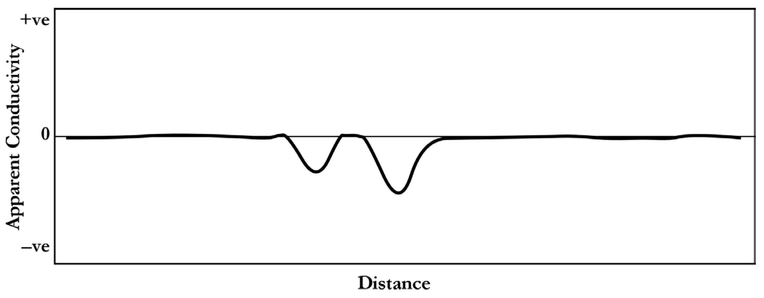
The MRB filter is a slightly modified version of the rolling ball algorithm, where the ball is run above the 3D surface instead of underneath it. The result of applying the MRB filter to the data presented in Figure 5 is shown in Figure 6. The MRB filter is successful in removing both the gradual change in background apparent conductivity, as well as the positive wings of the TCM anomalies, resulting in a relatively flat line with 2 small negative troughs pointing directly to the causative utilities, as shown in Figure 2A.

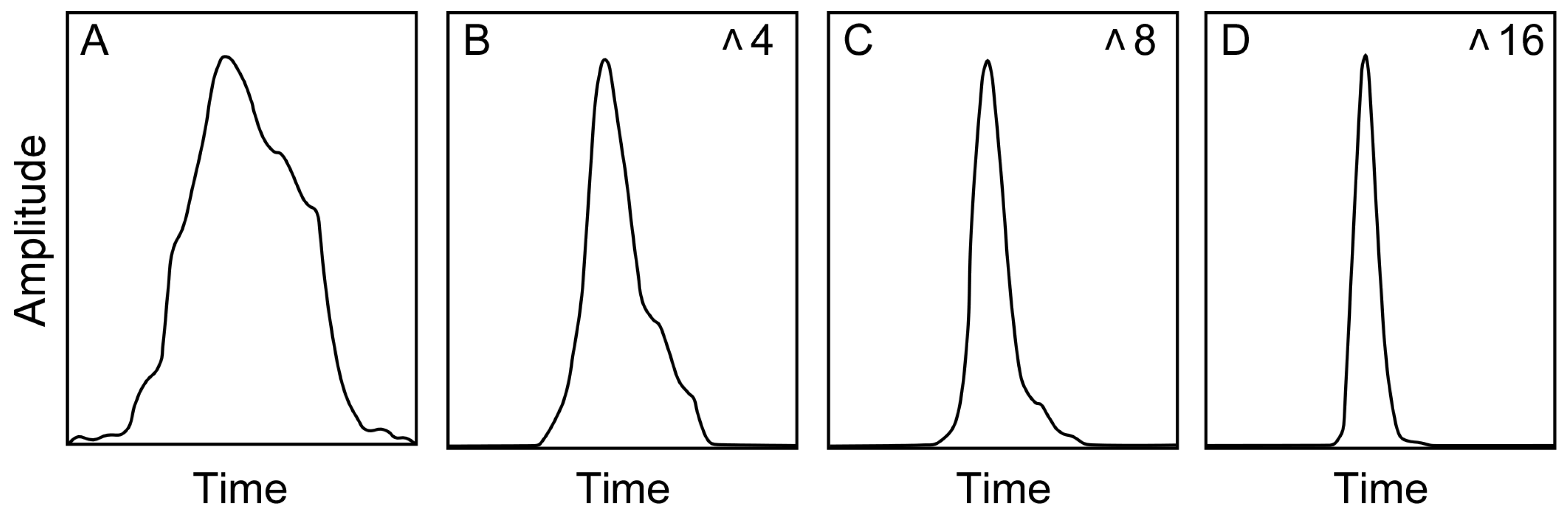
The third step is to apply the virtual resolution enhancement (VRE) filter to sharpen these anomalies and remove any irregularities in their shapes. The VRE filter was proposed by Rashed and Atef in 2020 to enhance the virtual resolution of seismic data [35]. However, it can be used in the proposed triple filter as a final stage that sharpens the negative peak of the apparent conductivity curve to pinpoint the causative utility. The foundation of the VRE filter is in the simple mathematical principle that, when raised to any power, one stays constant, while decimal digits result in decimal digits with smaller values that decrease as the power value increases. This simple principle can be applied to sharpen and remove distortion from any wavelet, as explained in Figure 7. Converting the distorted and wide troughs into sharp and spatially limited ones helps the interpretation of the apparent conductivity maps, especially in complex areas.

Figure 7A is a positive component of a typical distorted wavelet. This wavelet is normalized by dividing all its samples by its peak amplitude value, which sets its peak value to one and the rest of the samples to decimal digits. When all the sample values are raised to a power, except for the peak value that remains constant, all sample values decrease with increasing power.

Applying this straightforward procedure to the wavelet depicted in Figure 7A at powers of 4, 8, and 16 yields the results illustrated in Figure 7B, Figure 7C, and Figure 7D, respectively. Then, by multiplying each sample of the resulting wavelet by the initial peak amplitude value, the wavelet’s original amplitude can be restored, while the acquired virtual resolution enhancement is preserved. This procedure facilitates easier and more precise interpretation of utility locations on the apparent conductivity maps.

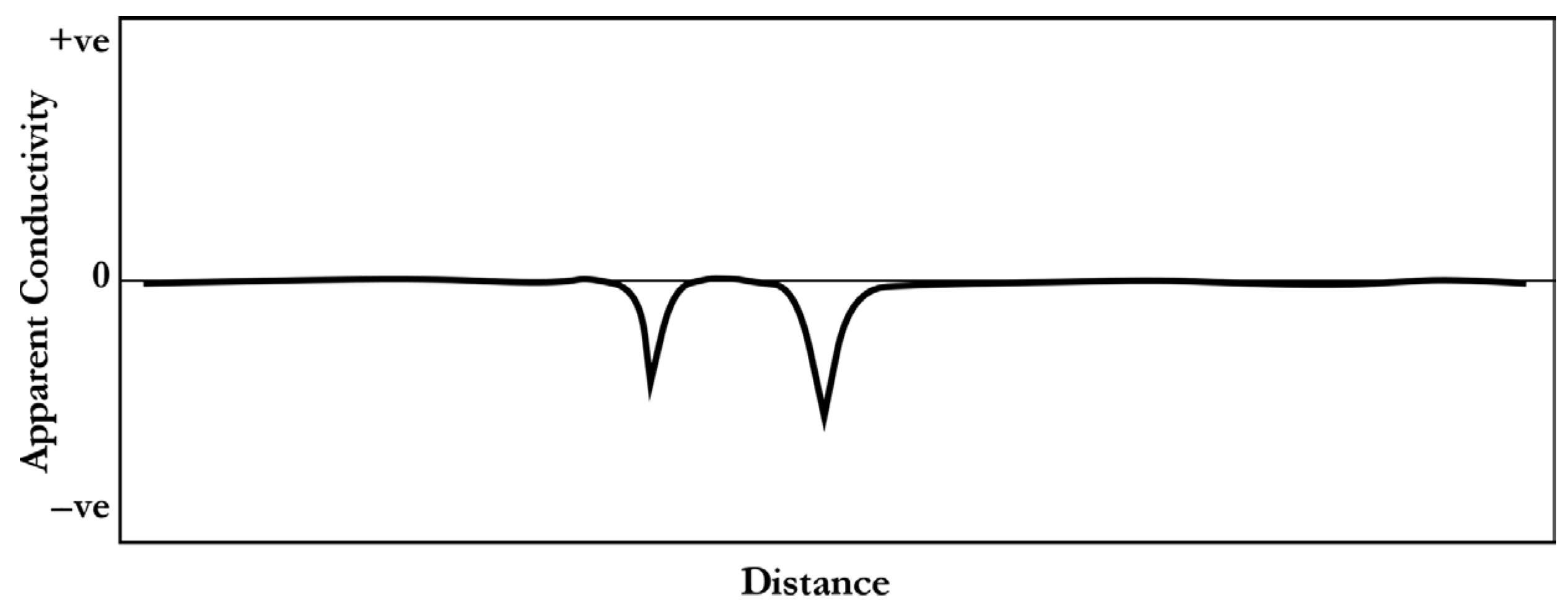
Figure 8 shows the result of applying the VRE filter to the data presented in Figure 6. The result clearly shows that the negative peaks have become sharper and pinpoint the exact location of the causative underground utilities.

The previously explained 3 steps should attenuate some of the most nagging issues with TCM data and result in a sharp negative peak(s) pointing directly to the causative utilities. This can be a small step in paving the way toward an automated process for real-time delineation of underground utilities. The following section shows the results of applying this triple filtering routine to different field datasets collected using different TCMs in different environments to prove the validity of the proposed filter.

3. Results and Discussion

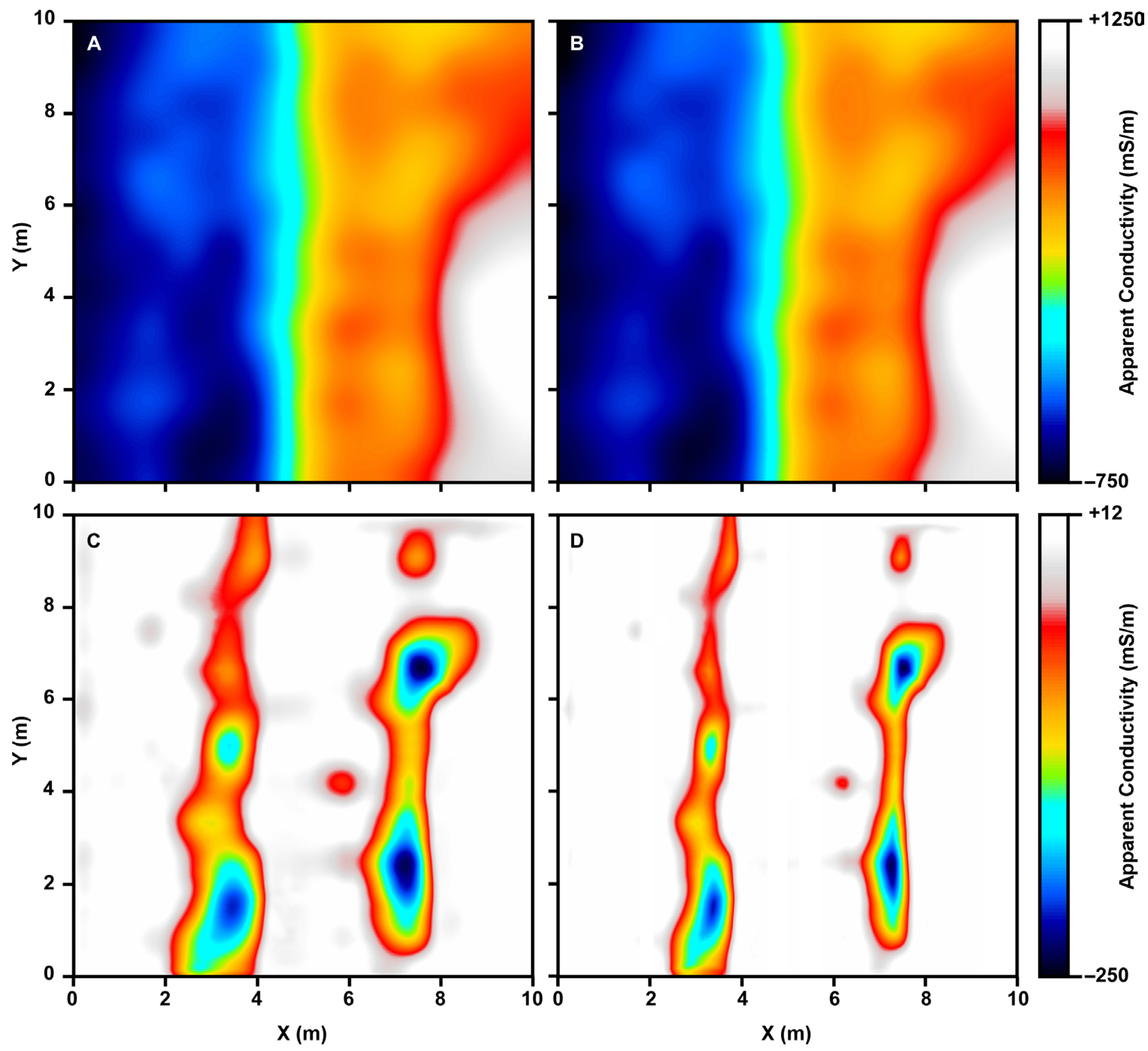
In this section, we present the results of applying the triple filter to the previously mentioned four datasets, explain its effect on the apparent conductivity maps, and discuss the enhancement the triple filter brings to the processed data. The first test data, collected in Dammam City, are gridded with 100 points per meter in both directions, resulting in a 1000 by 1000 node grid. The data are then plotted as a contour map (Figure 9A) and then treated with the SG filter with a window size of 75 samples and a polynomial degree of 3 (Figure 9B). The MRB filter is applied to data with a ball radius of 55 nodes (Figure 9C). The output of the MRB filtering process is then treated with the VRE filter, using a window size of 81 and a power of 4. The result of the triple filtering process is displayed in Figure 9D.

The result of the triple filtering clearly shows the presence of two large pipelines running parallel to each other from the top to the bottom axes of the map. The first one intersects with the x-axis of the map at x = 3 m, and the second is at x = 7.5 m. The presence of these two underground pipelines, separated by a distance ranging from 4 to 5 m, coincides well with prior information, and the survey aimed at delineating their exact locations. However, due to the presence of a surface concrete wall as well as other stationary and mobile sources of noise, the original map provides little, if any, information at all about the exact location of these pipelines. The map shows gradual variation in apparent conductivity from −750 milli-Siemens per meter (mS/m) near the left edge of the map to +1250 mS/m near the right edge. On the contrary, the output of the triple filtering process, although far from perfect, pinpoints the exact locations of the pipelines with two parallel narrow zones of apparent conductivity ranging between −250 and −50 mS/m embedded in a background of about 0 mS/m (Figure 9D).

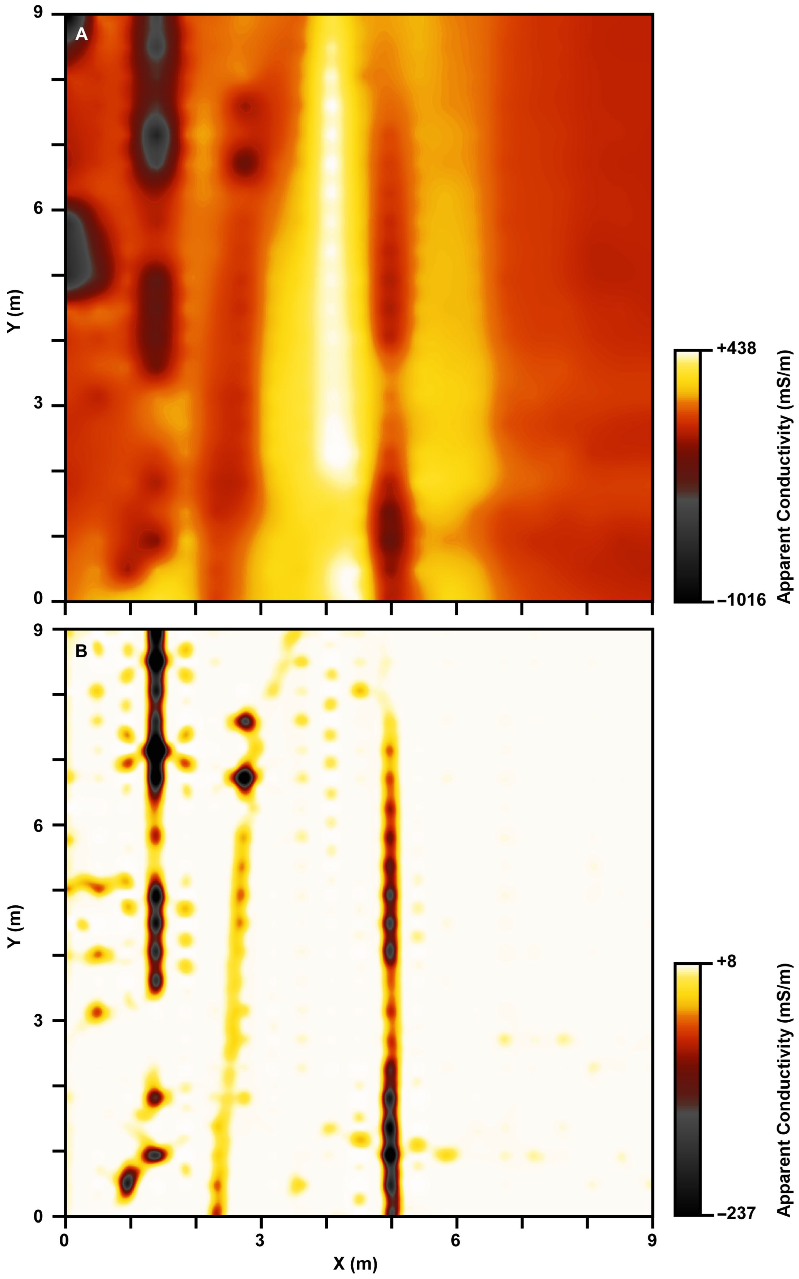
The second test dataset, collected in the Jubail Industrial Complex, is gridded, and the proposed triple filtering is applied to these data with an SG filter window size of 60 and a polynomial degree of 4. The MRB radius is 42 nodes, and the power of the VRE is 5. The interference of three semi-parallel underground utilities, in addition to the presence of two large sources of noise near the left axis of the map at y = 5.5 and 9 m, creates a vague and complex apparent conductivity map whose interpretation is quite challenging, if not impossible (Figure 10A).

Apparent conductivity values fluctuate between −1016 and +438 mS/m on the original map. On the other hand, the result of the triple filtering process indicates the exact location and extension of the three utilities at x = 1.0, 2.5, and 5 m, in a manner that makes interpretation as easy as drawing straight lines (Figure 10B). These three anomalies have apparent conductivity values ranging between −6 and −237 mS/m, lying within a background of almost 0 mS/m. This is a good example of unveiling and separating hidden and interfering anomalies caused by utilities adjacent to other utilities (Figure 10B).

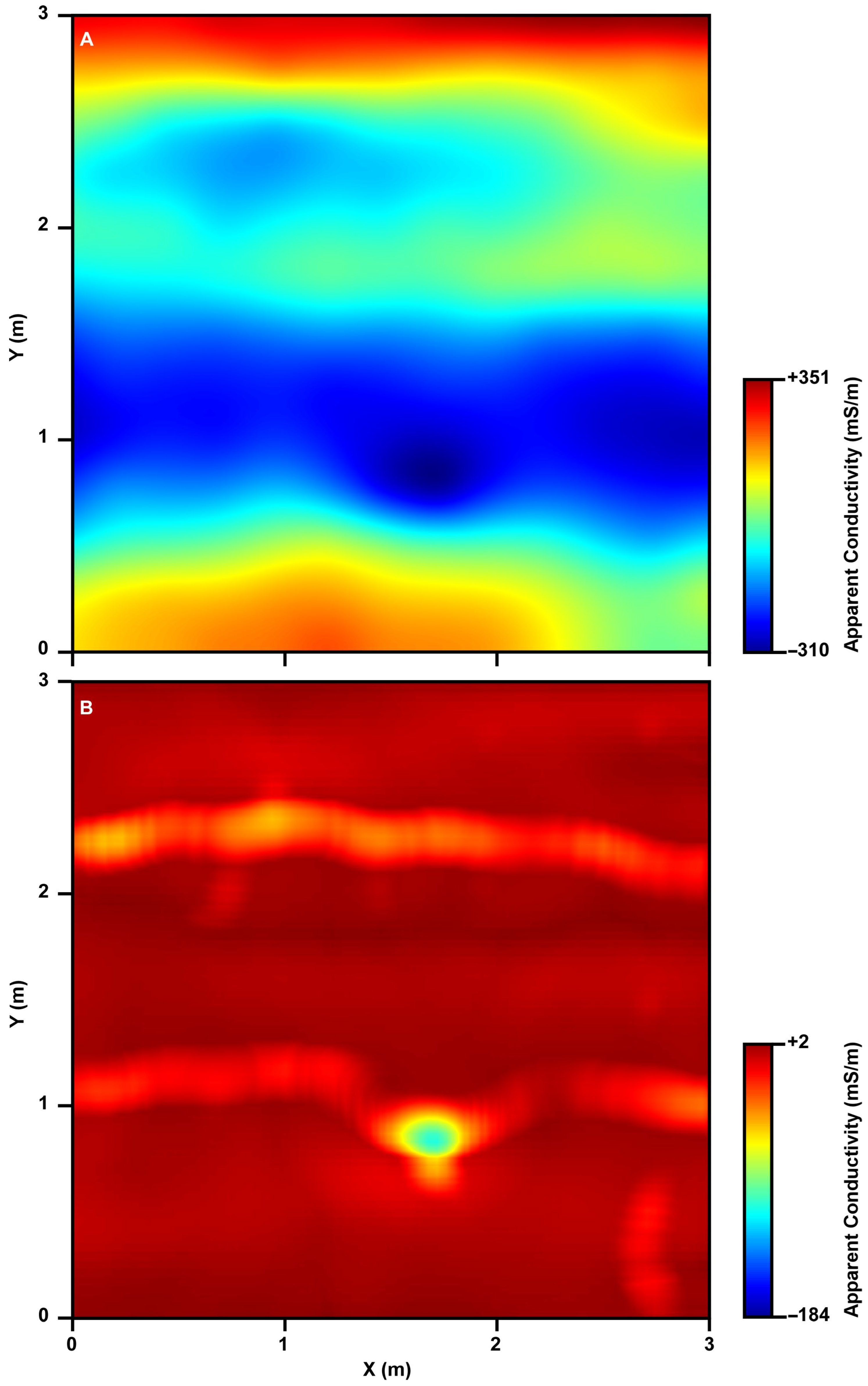
The gridded and plotted map of the third test dataset, collected in Mecca City, shows smeared and interfering apparent conductivity anomalies (Figure 11A). No useful information about the location or the direction of the causative underground utilities can be extracted from this map.

The original map shows horizontally elongated zones of apparent conductivity ranging between −310 and +350 mS/m. In the triple-filtered apparent conductivity data, however, the map evidently shows two crocked utilities running parallel to the x-axis of the map and crossing the y-axis at 1 and 2.2 m marks (Figure 11B).

The apparent conductivity of these two crocked anomalies ranges between −20 and −40 mS/m. However, the utility crossing the y-axis at the 1 m mark has a high apparent conductivity amplitude spot of nearly −150 mS/m near its middle. Excavation at this site reveals the presence of two identical insulated copper power cables buried exactly underneath the revealed anomalies shown in Figure 11B. Each of these power cables is 10 cm in diameter and slightly crooked. Moreover, the excavation shows that the lower power cable sticks up and gets closer to the ground surface, exactly where the high-amplitude anomaly is depicted.

This example shows the great capability of the proposed triple filtering routine to extract useful information about underground utilities from complex apparent conductivity maps with interfering anomalies coming from neighboring utilities. It also shows the ability of such a routine to reveal precise images of the underground, delineating not only their exact locations but also their shapes and depths.

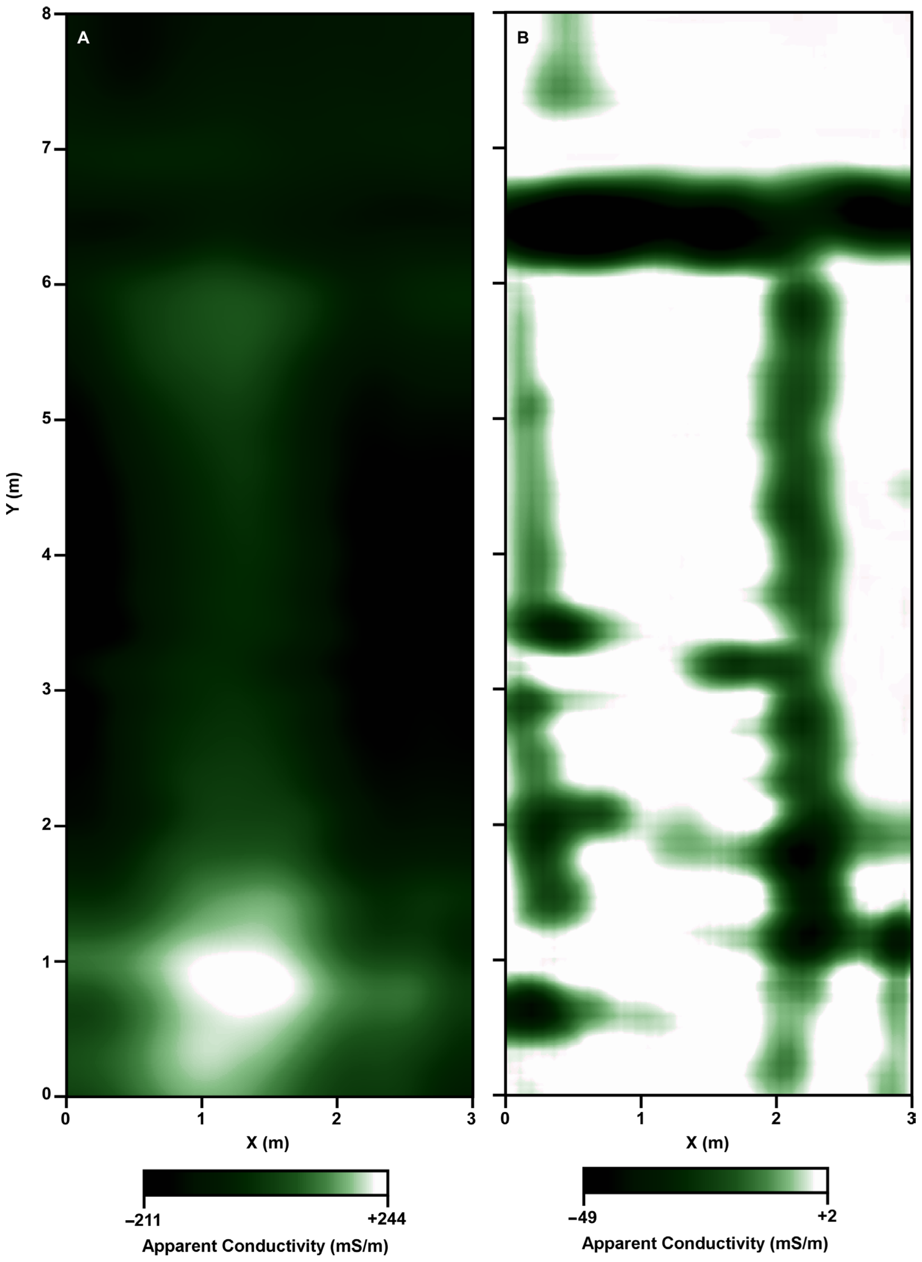
The last test dataset, acquired in the heart of the noisy and crowded Jeddah City, shows nothing but a blurred image of irregular variation in the apparent conductivity values fluctuating between −211 and +244 mS/m in irregular regions covering the entire map (Figure 12A). In contrast, the triple-filtered map clearly shows a strong linear anomaly with an apparent conductivity of −49 mS/m, running parallel to the x-axis between 6 and 7 m marks on the y-axis. In addition, the map also shows two perpendicular weaker linear anomalies, probably caused by two utilities running parallel to the y-axis near the left and right borders of the map (Figure 12B). All these anomalies are embedded with background apparent conductivity around 0 mS/m, covering the rest of the map (Figure 12B).

The example in Figure 12 is clear evidence of the capability of the proposed triple filtering routine to acquire useful and precise information from a complex apparent conductivity map, which contains interfering anomalies from utilities of different characters or sizes running in different directions and yielding a clear apparent conductivity map that is interpretable.

These four examples of applying the proposed triple filter to a diverse group of apparent conductivity maps demonstrate that the triple filter can bring about a significant enhancement to the maps (Figure 9, Figure 10, Figure 11 and Figure 12). The triple filter not only exposed anomalies masked by background apparent conductivity variation but also disentangled overlapping and interfering complex anomalies caused by the presence of utilities buried close to each other. Moreover, the diversity of the examples demonstrated that the triple filtering process can treat data collected using different TCMs with different data acquisition modes, over different utilities, in different environments.

The first example was good evidence of the triple filter’s capability to attenuate the effect of irrelevant conductive objects that create massive apparent conductivity variations, masking the anomalies caused by the targeted utilities (Figure 9). The second example clearly showed that the triple filter was able to separate interfering anomalies caused by neighboring utilities (Figure 10). This particular power of the triple filter is of great importance because closely spaced utilities are common in most urban areas. In the third example, the proposed triple filter was capable of not only revealing and delineating the exact location of the utilities but also showing some essential characteristics of underground utilities, such as their shape and depth (Figure 12). This particular site was later excavated, and the interpreted type, shape, and depth of the depicted utilities were confirmed.

The fact that the three consecutive steps of the proposed triple filter are characterized by simplicity and a light computational load, and given the continuous increase in the computation capability and decrease in hardware sizes, this proposed triple filter may lay the foundation for integrating such a process as a built-in tool in future TCMs to allow for real-time detection and characterization of underground utilities.

The only obstacle facing such a possibility is selecting the processing parameters. These parameters include the window size and polynomial degree of the SG filter, ball radius for the MRB filter, and window size and power for the VRE filter. Selecting the optimum filtering parameters can be tricky and needs fine-tuning to achieve the best results. However, if an attempt is ever made to include the triple filtering process in the data acquisition devices, these parameters can be adjusted in the field along with the calibration process, which is mandatory because of the site-dependent nature of terrain conductivity data.

Overall, it can be confidently claimed that the proposed triple filter successfully solved some of the most persistent problems related to apparent conductivity measurements and, as a result, could reveal and delineate underground utilities hidden in complicated apparent conductivity maps.

4. Conclusions

The triple filtering routine is a process that has helped in reducing some of the most common issues related to apparent conductivity measurements. These issues include complex anomaly shapes and interference, random noise caused by TCM tilting and rotation, and irrelevant large objects affecting the collected data. By applying this triple filtering routine, namely the SG filter, the MRB filter, and the VRE filter, to various apparent conductivity datasets with different characteristics, it has been proven that this routine can accurately delineate masked underground utilities and provide good information about their characteristics and extensions. This routine can be considered as a small step toward developing a new generation of TCMs with new capabilities that include instant delineation and characterization of underground utilities.