Application of Machine Learning Methods for Gravity Anomaly Prediction

Abstract

Gravity anomalies play critical roles in geological analysis, geodynamic monitoring, and precise geoid modeling. Obtaining accurate gravity data is challenging, particularly in inaccessible or sparsely covered regions. This study evaluates machine learning (ML) methods—Support Vector Regression (SVR), Gaussian Process Regression (GPR), and Ensemble of Trees—for predicting gravity anomalies in southeastern Kazakhstan and compares their effectiveness with traditional Kriging interpolation. A dataset, consisting of the simple Bouguer anomaly values, latitude, longitude, elevation, normal gravity, and terrain corrections derived from historical maps at a scale of 1:200,000, was utilized. Models were trained and validated using cross-validation techniques, with performance assessed by statistical metrics (RMSE, MAE, R²) and spatial error analysis. Results indicated that the Exponential GPR model demonstrated the highest predictive accuracy, outperforming other ML methods, with 72.9% of predictions having errors below 1 mGal. Kriging showed comparable accuracy and superior robustness against extreme errors. Most prediction errors from all methods were spatially associated with mountainous regions featuring significant elevation changes. While this study demonstrated the effectiveness of machine learning methods for gravity anomaly prediction, their accuracy decreases in complex terrain, indicating the need for further research to improve model performance in such environments.

1. Introduction

Gravity anomalies, particularly Bouguer anomalies, are essential for analyzing geological structures [1,2,3,4], monitoring geodynamic processes [5,6], and addressing geodetic challenges [7,8]. They play crucial roles in modeling the gravimetric geoid [9,10], which is fundamental for precise geodetic measurements and Earth science applications. According to Hofmann-Wellenhof and Moritz [11], determining the geoid surface is based on solving the boundary value problem presented by Stokes’ formula. The practical implementation of this formula requires a globally distributed and dense coverage of terrestrial gravity data.

However, obtaining high-density gravity data in various environments remains a challenging task. This challenge arises not only from accessibility constraints in study areas, but also from the high costs associated with conducting gravimetric surveys. Previous studies [12,13] have highlighted that the high costs associated with equipment procurement, survey implementation, and data processing significantly limit the availability of dense gravity data. Another fundamental requirement for constructing a gravimetric geoid is the uniform spatial distribution of gravity observations with a specified resolution, which is technically difficult to achieve. Consequently, interpolation methods are commonly employed to construct a regular grid. The choice of an optimal approach for data point density and interpolation methods is a key issue in this context.

Classical interpolation techniques, such as Kriging, continuous curvature splines, and least squares interpolation in tension (LCS), are widely used for gap-filling and densification of gravimetric data points, yielding varying levels of accuracy [14]. The spline method is applied when data points are uniformly distributed with smooth variations in values. LCS is utilized for datasets with heterogeneous point density, integrating correlation information. As one of the most widely used interpolation methods, Kriging estimates the value at an unknown location by computing a weighted average of the nearest data points. This approach contributes to reducing inversion uncertainty and enhancing spatial resolution. Kriging outperforms many other interpolation techniques, providing higher accuracy in interpolated values [15,16]. Each of the traditional interpolation methods has its advantages; however, their accuracy is highly dependent on the density of gravimetric data. Moreover, traditional interpolation methods face significant challenges in regions with steep gravity gradients, as their underlying assumptions of spatial continuity become less reliable. In regions with sparse gravity data coverage, these methods may introduce significant errors in gravity value predictions.

Currently, many machine learning algorithms enable the prediction of process dynamics, the identification of hidden patterns, the filling of data gaps, and the enhancement of model accuracy across various scientific and applied domains. The rapid advancement of artificial intelligence has introduced new opportunities for data forecasting [17,18]. Several studies [19,20,21] have explored the application of machine learning (ML) methods for gravity data prediction, demonstrating superior forecasting accuracy compared to traditional approaches. Liu et al. [22] demonstrated that the Random Forest (RF) and recurrent neural network (RNN) algorithms achieved the highest accuracy in predicting gravity data, outperforming the Support Vector Machine (SVM) and Kriging methods. Specifically, for large-scale datasets, Random Forest and RNN achieved the best results, with Root Mean Square Error (RMSE) values of 2.7438 and 3.4804, respectively. For small-scale datasets, the corresponding RMSE values were 7.6032 and 8.6699. In a separate study, performed by Tierra and De Freitas [23], the Artificial Neural Network (ANN) model effectively predicted Free-Air Gravity Anomalies with high accuracy. The model achieved a Standard Deviation (SD) of 0.241, significantly outperforming traditional interpolation methods, such as Kriging (SD: 21.476) and Minimum Curvature (SD: 20.264), by capturing complex spatial relationships in the gravity data. In this study, we evaluate the effectiveness of three ML algorithms for gravity data interpolation: Support Vector Regression (SVR), Ensembles of Trees, and Gaussian Process Regression (GPR). These algorithms were selected based on their specific advantages: SVR is effective for small datasets with nonlinear patterns, Ensembles of Trees is robust against data noise and overfitting, and GPR is capable of quantifying prediction uncertainty.

The use of machine learning offers an advance in gravity data prediction by improving the accuracy of interpolation in regions with sparse or irregular measurements and capturing complex spatial relationships that are often not well represented by classical methods. These capabilities make machine learning a promising tool for enhancing the reliability and accuracy of gravity data, which serve as a critical foundation for subsequent studies in geodesy, geophysics, geology, and related Earth science disciplines.

The objectives of this study are to identify the most effective machine learning methods for predicting gravimetric data and to provide a comprehensive comparison of the predicted values with the traditional Kriging interpolation method.

This research is particularly relevant in the context of developing a regional geoid model for Kazakhstan as part of a national project, which aims to enhance the accuracy of geodetic measurements and establish a foundation for future gravimetric investigations. To the best of our knowledge, this is the first study to explore the applicability of ML algorithms for gravity data prediction in Kazakhstan’s territory. The obtained results will contribute to the development of a scientific and methodological framework for selecting optimal approaches to improving the accuracy of Kazakhstan’s geoid model.

2. Materials and Methods

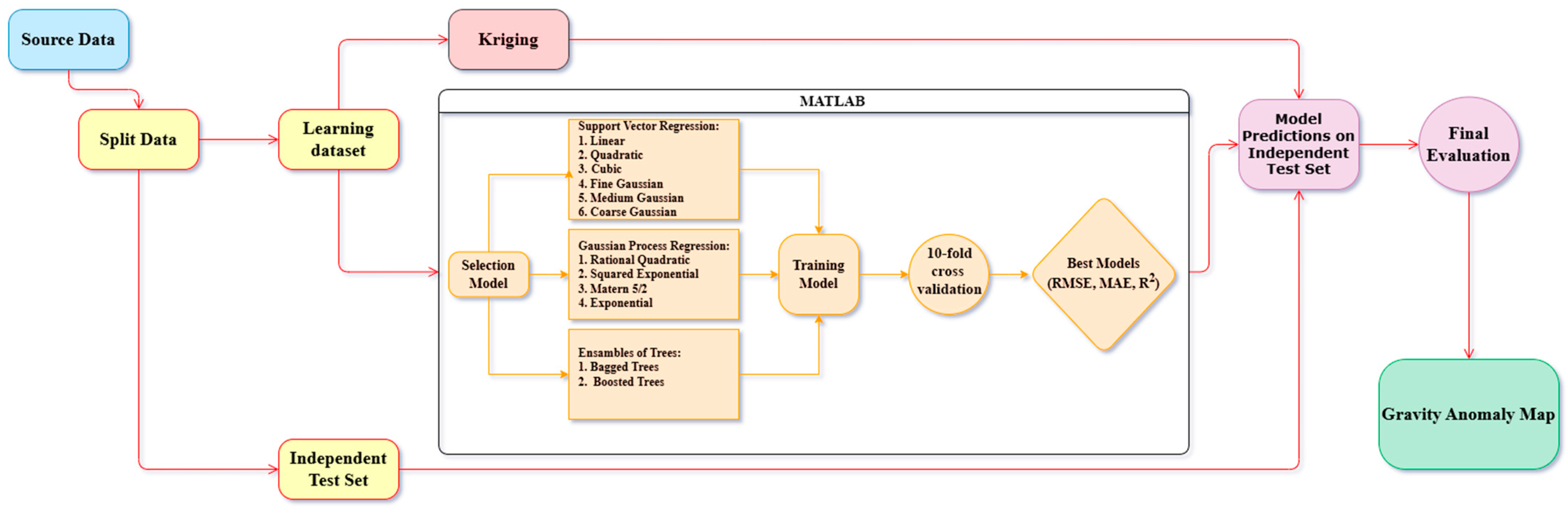
Figure 1 presents a flowchart outlining the methodology implemented in this study. The workflow encompasses multiple stages, including data preprocessing, model selection, training, validation, and final performance evaluation. The study area and dataset are described in Section 2.1, the validation process in Section 2.2, and the machine learning and interpolation methods in Section 2.3, Section 2.4, Section 2.5 and Section 2.6. The results, along with their interpretation, are discussed in Section 3.

The flowchart illustrates the application of machine learning methods for predicting gravity anomalies. The first stage involved data preparation, wherein the initial dataset was divided into the two following subsets:

-

Learning dataset—used for model training and validation;

-

Independent test set—randomly distributed across the study area for final evaluation and comparison with traditional interpolation method.

Data preprocessing included feature normalization to ensure consistent contribution from input features (latitude, longitude, elevation, normal gravity). Regression modeling was performed using the MATLAB^® environment (version R2024a). Hyperparameter optimization within Regression Learner was conducted automatically using built-in Bayesian optimization methods. This automated procedure systematically explored optimal hyperparameter combinations to minimize model error (RMSE, MAE), thus enhancing predictive accuracy and model generalization. Additionally, 10-fold cross-validation was employed to robustly evaluate model performance and mitigate potential overfitting. Once preprocessed, the dataset was used to train different ML models, including Support Vector Regression (SVR), Gaussian Process Regression (GPR), and Ensembles of Trees, as well as the traditional Kriging interpolation method. For SVR, the following six different kernel functions were tested: Linear, Quadratic, Cubic, Fine Gaussian, Medium Gaussian, and Coarse Gaussian.

Each kernel function was evaluated to determine the best-performing configuration. Similarly, four kernel types were examined for GPR, including Rational Quadratic, Squared Exponential, Matern 5/2, and Exponential. For Ensemble of Trees, both Bagged Trees and Boosted Trees were implemented. Subsequently, model selection was conducted to identify the most suitable algorithm for prediction. The training phase included hyperparameter tuning and optimization using 10-fold cross-validation, which helped to assess model stability and generalization performance. The best-performing model was determined based on statistical error metrics, including Root Mean Square Error (RMSE), Mean Absolute Error (MAE), and the Coefficient of Determination (R²).

Following the selection of the best-performing models from each tested approach (SVR, GPR, and Ensembles of Trees), a final independent test set evaluation was performed. The best-selected models were compared against Kriging to assess their effectiveness in predicting gravity anomalies.

The final stage involved the interpretation of results, wherein the predicted data were visualized through maps, histograms, and graphs. This visualization facilitates a detailed spatial analysis of prediction errors, the identification of underlying patterns, and the delineation of regions with the highest levels of uncertainty in gravity anomaly predictions.

2.1. Study Area and Dataset

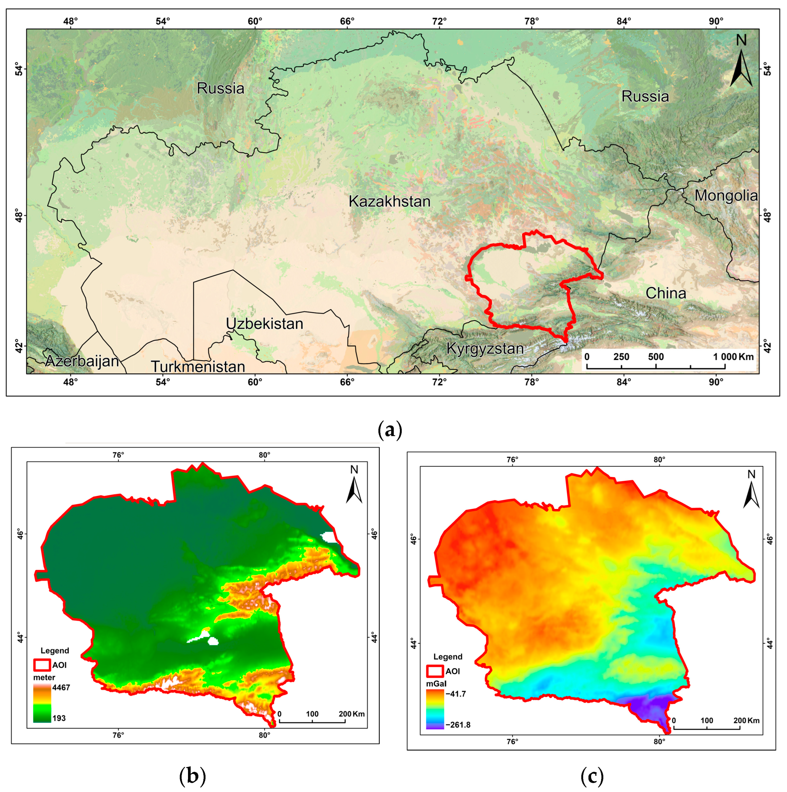
The study area is located in southeastern Kazakhstan, within the coordinates 42°25′–47°20′ N and 73°43′–82°10′ E (Figure 2a). This region encompasses a diverse range of topographic and geological features, including the mountainous terrain of the Tian Shan and Zhetysu Alatau ranges, as well as extensive lowland deserts, providing an ideal setting for gravity field analysis.

The topography of the study area exhibits significant variability: the northern part is dominated by vast desert landscapes, while the southeastern section is occupied by the Tian Shan and Zhetysu Alatau mountain ranges. Elevations range from 302 m to 4540 m (Figure 2b). The presence of both flat and mountainous terrains allows for an assessment of machine learning model accuracy under varying geographic conditions, offering insights into their efficiency in forecasting gravity field anomalies.

The gravity field of the study area demonstrates pronounced spatial variability, primarily influenced by geological structure and regional topography. The map of the simple Bouguer anomalies (Figure 2c) reveals significant contrasts in gravity anomalies, ranging from −41.7 mGal to −261.8 mGal. These variations reflect the heterogeneous subsurface composition, including differences in crustal density, major fault zones, and sedimentary basin distributions. The presence of such complex anomalies underscores the necessity of advanced interpolation techniques capable of accurately capturing gravity field variations across diverse landscapes.

As shown in

Table 1. Input data for learning and testing sets.

Input Data	Learning Dataset			K-Cross Validation	Independent Test Set
	Min	Max	Count	Value	Min	Max	Count
latitude, degree	42.420	47.318	12,390	10	42.439	47.306	2641
longitude, degree	74.103	82.168	12,390	10	74.106	82.141	2641
H (normal), m	302.00	4469.00	12,390	10	320.5	4537.6	2641
G0, mGal	980,368.8	980,811.5	12,390	10	980,370.5	980,810.4	2641
BA, mGal	−262.2	−41.0	12,390	10	−259.2	−41.9	2641

, the dataset used for training and testing the selected models consists of 15,031 points with known values of latitude, longitude, elevation (H), normal gravity (G₀), and simple Bouguer anomaly (BA). Although terrain correction values were present in the original dataset, they were not included in the training dataset, as the correction was unavailable for the entire study area (terrain correction values were available for 6949 out of 15,031 total points). Nevertheless, these values were utilized in a supplementary analysis. An additional correlation analysis was performed between the model prediction errors and the terrain correction values at known locations, in order to assess their potential association with the spatial distribution of the errors. The elevation values are referenced in the Baltic Height System, and the coordinates are in the WGS 84 reference system. The spatial distribution density of the points is approximately 5 km.

Both the Digital Elevation Model (DEM) and the ground-based gravity observations were obtained through the vectorization of historical topographic and gravimetric maps of the USSR at a scale of 1:200,000, as part of the “Development of a geoid model of the Republic of Kazakhstan as the basis of a unified state coordinate system and heights” project.

2.2. Validation and Performance Metrics

The evaluation of machine learning model performance is conducted based on standard error metrics, which quantify the discrepancy between predicted and actual values. The following metrics are used:

The Root Mean Square Error (RMSE) measures the Standard Deviation of prediction errors, giving higher weight to larger errors, as follows:

$$RMSE=\sqrt{{\displaystyle \frac{1}{n}}\sum _{ i=1}^n\left|A_i-F_i \right|}$$

(1)

The Mean Absolute Error (MAE) calculates the average absolute difference between predicted and actual values, providing a straightforward measure of prediction accuracy, as follows:

$$MAE={\displaystyle \frac{1}{n}}\sum _{i=1}^n\left|A_i-F_i\right|$$

(2)

The Coefficient of Determination (R²) assesses how well the predicted values fit the actual observations, indicating the proportion of variance as explained by the following model:

$$R^2\left(A,F\right)=1-{\displaystyle \frac{{\sum }_{i=1}^n({F_i-A_i)}^2}{{\sum }_{i=1}^n({F_i-\overline{F_i})}^2}}$$

(3)

In these Equations (1)–(3), $n$ represents the number of observation samples, $A_i$ denotes the predicted value for the i-th observation, and $F_i$ represents the actual value.

These metrics provide a comprehensive assessment of model performance, capturing both accuracy and variability. By analyzing them, we can identify the models that demonstrated superior predictive accuracy. The comparison of machine learning models with traditional Kriging interpolation was performed using these metrics to ensure a robust evaluation of their predictive capabilities.

2.3. Support Vector Regression

Support Vector Regression (SVR) is a supervised learning approach that identifies an optimal hyperplane to predict continuous values while allowing for a margin of tolerance defined by the ε-insensitive loss function. Unlike the classical Support Vector Machine (SVM), used for classification tasks, SVR seeks to fit a function that minimizes deviations beyond a defined ε-margin while penalizing larger errors. Mathematically, this optimization problem can be expressed as follows [24]:

$$\underset{\omega ,\mathit{b},\xi , {\xi }^{*}}{\mathit{min}}{\displaystyle \frac{1}{2}}{‖w‖}^2+C\sum _{i=1}^n\left({\xi }_i+{\xi }_i^{*}\right)$$

(4)

Subject to the following:

$$\begin{array}{c}{y}_i-〈w, x_i〉-b \le ϵ+{\xi }_i\\ 〈w, x_i〉+b-y_i\le ϵ+{\xi }_i^{*}\\ {\xi }_i, {\xi }_i^{*} \ge 0\end{array}$$

In Equation (4), $w$ represents the weight vector of the model, b is the bias term, ${\xi }_i, \mathrm{a}\mathrm{n}\mathrm{d} {\xi }_i^{*}$ are slack variables that allow for errors beyond the ϵ-margin, $C$ is the regularization hyperparameter, controlling the trade-off between model generalization and prediction accuracy, and $ϵ$ is the insensitive zone, where errors are not penalized. This allows the model to balance prediction accuracy and generalization capability.

The model’s performance is highly dependent on the choice of kernel function, which determines how the input data are mapped into a higher-dimensional space. In this study, six kernel functions—Linear, Quadratic, Cubic, and three variations of the Gaussian Radial Basis Function (RBF) kernel (Fine, Medium, and Coarse)—were tested to identify the most suitable SVR configuration for gravity anomaly prediction.

For nonlinear datasets, a kernel trick is applied to transform the input data into a higher-dimensional space where a linear separation becomes feasible. One of the most commonly used kernels for this purpose is the Radial Basis Function (RBF), or Gaussian kernel, which has demonstrated high effectiveness in regression tasks by modeling complex relationships between input variables [25,26,27].

2.4. Ensembles of Trees

Ensemble learning methods improve predictive performance by combining multiple models to reduce variance and bias. These methods are particularly effective in regression tasks where complex relationships exist within the data. The fundamental formula representing the working principle of the method is as follows [28]:

$$f^M (x)=\sum _{k=1}^M{w}_k{f}_k\left(x\right)$$

(5)

In Equation (5), $M$ represents the number of trees (or models) in the ensemble, $w_k$ denotes the weight of each tree, and $f_k(x)$ represents the prediction of an individual model; if all models are equally weighted, the weights are uniform, given by $w_k=1/M.$ The two primary ensemble techniques applied in this study are Bagged (Bootstrap Aggregation) and Boosted Trees.

Bagged Trees operate by training multiple decision trees on randomly resampled subsets (Bootstrap samples) of the original dataset. Each tree learns from a slightly different perspective of the data, and the final prediction is obtained by averaging the outputs of all trees. This approach significantly reduces variance and prevents overfitting, particularly in high-dimensional datasets. Additionally, Out-of-Bag (OOB) estimation allows model accuracy to be assessed without requiring a dedicated validation dataset, further enhancing robustness and computational efficiency [29,30].

In contrast, Boosted Trees build decision trees sequentially, where each new tree focuses on correcting the residual errors of the previous ones. This iterative refinement makes Boosting highly effective for complex regression problems. In this study, Least Squares Boosting (LSBoost), which optimizes the squared error at each step, was employed.

2.5. Gaussian Process Regression

Gaussian Process Regression (GPR) is a non-parametric Bayesian approach that models an unknown function as a distribution over possible functions that best fit the observed data. Unlike deterministic regression models, GPR provides both point estimates and uncertainty quantification, making it particularly useful for applications requiring confidence intervals in predictions. The Gaussian Process is defined as a joint probability distribution over any finite set of observations, as follows [31]:

$$p\left(y\right)=\mathcal{N}(m, K)$$

(6)

In Equation (6), m is the mean vector and K is the covariance matrix.

The elements of the mean vector and covariance matrix are obtained through the mean function $m\left(x\right)$ and the covariance function $k(x,x^{\prime }),$ respectively, as follows:

$$\begin{array}{c}{m}_i=m(x_i,\theta )\\ K_{ij}=k(x_i,x_j,\varphi )\end{array}$$

(7)

The key component of GPR is the covariance (kernel) function, which defines the degree of dependence between different input points. This function determines the smoothness and overall structure of the modeled function. If two input values are close in space, their corresponding function outputs are expected to be highly correlated, depending on the chosen kernel function [32].

The parameters of the covariance function typically include the characteristic length scale, which controls how quickly the function varies with changes in the input; the noise variance, which accounts for measurement noise; and the function variance, which defines the overall variability of the function. The selection of an appropriate kernel function is crucial for ensuring accurate predictions. In this study, multiple kernel types, including Squared Exponential, Matern 5/2, Exponential, and Rational Quadratic, were tested to determine the best configuration for gravity anomaly prediction.

2.6. Kriging

The Kriging method is a collection of statistical tools used to model spatial relationships between measured points to predict values and estimate uncertainty at unmeasured locations [33]. In Kriging, the predicted value at any given point is calculated as a linear combination of values obtained from measured points, each assigned an appropriate weight. The Kriging weights are determined to minimize the variance of the predicted values. These weights depend on the selected model, the distances between measured and predicted points, and the overall spatial structure of the data distribution. Ordinary Kriging is an interpolation method that assumes stationarity of the random process with a known semi-variogram and an unknown but constant mean value, which is either estimated or ignored to ensure an unbiased estimate.

In spatial analysis, three functional models are widely used: spherical, exponential, and Gaussian. In this study, the spherical model was chosen, represented by the following equation:

$$\begin{array}{c}\gamma (h)= c_0+c\left\{{\displaystyle \frac{3h}{2r}}-{\displaystyle \frac{1}{2}}{\left({\displaystyle \frac{h}{r}}\right)}^3 \right\} for \mathit{0} < h \le r ,\\ =c_0+c for h>r \\ =\mathit{0} for h = \mathit{0}\end{array}$$

(8)

In Equation (8) c represents the spatially correlated variance, r is the correlation range, and $c_0$ + c is known as the “sill” [34].

3. Results

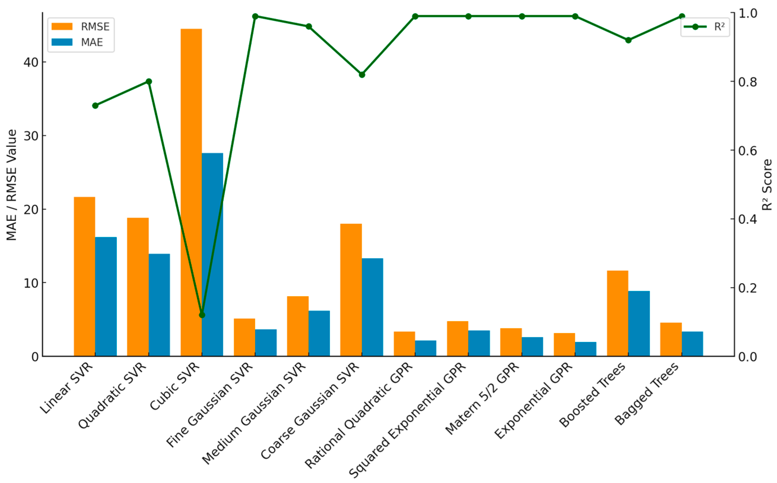
Based on the evaluation of performance metrics (Figure 3), the best-performing models were selected within each of the following method categories: Fine Gaussian SVR among Support Vector Regression (SVR) models; Exponential GPR among Gaussian Process Regression (GPR) models; and Bagged Trees among the ensemble methods, which included both Boosted Trees and Bagged Trees.

The best-performing models, along with Kriging, were applied to validate the independent test set, ensuring a comprehensive assessment of their effectiveness in predicting gravity anomalies. As shown in

Table 2. Performance of the tested models.

Method	MAPE (%)	MAE (mGal)	RMSE (mGal)	R2 (%)
Fine Gaussian SVR	3.5	3.5316	4.8645	0.9
Kriging	1.0269	1.0686	2.5948	0.9
Bagged Trees	2.6	2.5963	3.5562	0.9
Exponential GPR	0.9	0.98585	2.3042	0.9

, the Exponential Gaussian Process Regression (GPR) model achieves the best results across all key statistical metrics, confirming its effectiveness in predicting gravimetric data. The Fine Gaussian SVR and Bagged Trees models exhibited the highest errors in MAPE, MAE, and RMSE metrics, indicating their low predictive performance in this context. The Kriging method produced results nearly equivalent to Exponential GPR, further validating its efficiency in interpolation tasks.

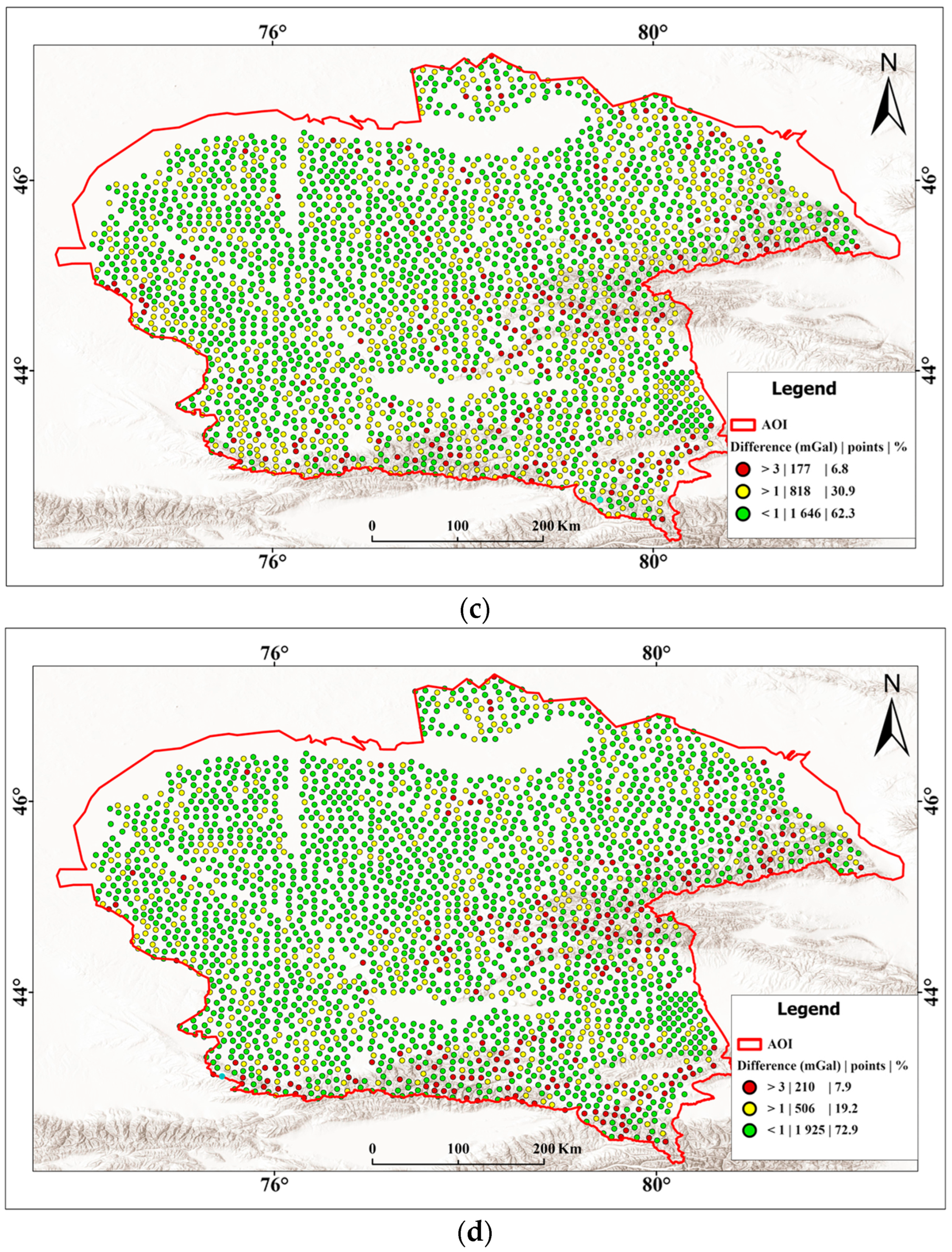
To evaluate the effectiveness of different methods for predicting the simple Bouguer anomalies, a test dataset was used, with its spatial distribution presented in Figure 4. The errors were classified into the following three categories:

• Large errors (>3 mGal, red points);
• Medium errors (1–3 mGal, yellow points);
• Small errors (<1 mGal, green points).

According to Denker [35], a prediction accuracy of approximately 1 mGal is generally considered sufficient to achieve a 1 cm geoid model. This threshold, thus, serves as a scientifically supported baseline for distinguishing small errors that do not critically affect high-precision geoid computation.

The 1–3 mGal range (medium errors) represents deviations that may still be usable for certain regional or medium-resolution geoid modeling tasks, but could introduce noticeable distortions in high-accuracy applications, especially in areas with rough gravity fields.

Errors greater than 3 mGal (large errors) exceed the tolerance limits commonly accepted in precise geoid or gravity field modeling and are likely to reflect significant discrepancies or noise in the input data.

This classification helps not only to visually assess the spatial distribution of prediction errors, but also to evaluate the model’s suitability for various geodetic and geophysical applications.

The Fine Gaussian SVR model exhibited the highest proportion of large errors (45.6%). Based on the spatial distribution, it can be observed that the errors are evenly dispersed throughout the region, without a clear correlation with topographic features or Bouguer anomaly gradients.

The Bagged Trees model also exhibits significant prediction deviations, but to a lesser extent compared to Fine Gaussian SVR. The proportion of large errors is 22%, which is lower than that in Fine Gaussian SVR, but still relatively high. Unlike Fine Gaussian SVR, the spatial distribution of errors follows a discernible pattern—large errors are more frequently observed in the southern and eastern regions, where complex gravity gradients are present.

The Kriging method demonstrates significantly better performance compared to the Fine Gaussian SVR and Bagged Trees methods. The proportion of large error points is reduced to 6.8%, while the majority of points (62.3%) exhibit small errors (<1 mGal). The error distribution is more uniform, with fewer instances of major deviations. This confirms the high efficiency of the method when applied to geostatistical data.

The Exponential GPR model achieved the best performance among all the evaluated approaches. The concentration of points with errors exceeding 3 mGal is minimal (7.9%), while 72.9% of the points have errors below 1 mGal. Thus, Exponential GPR demonstrates high adaptability and stability in predicting Bouguer anomalies.

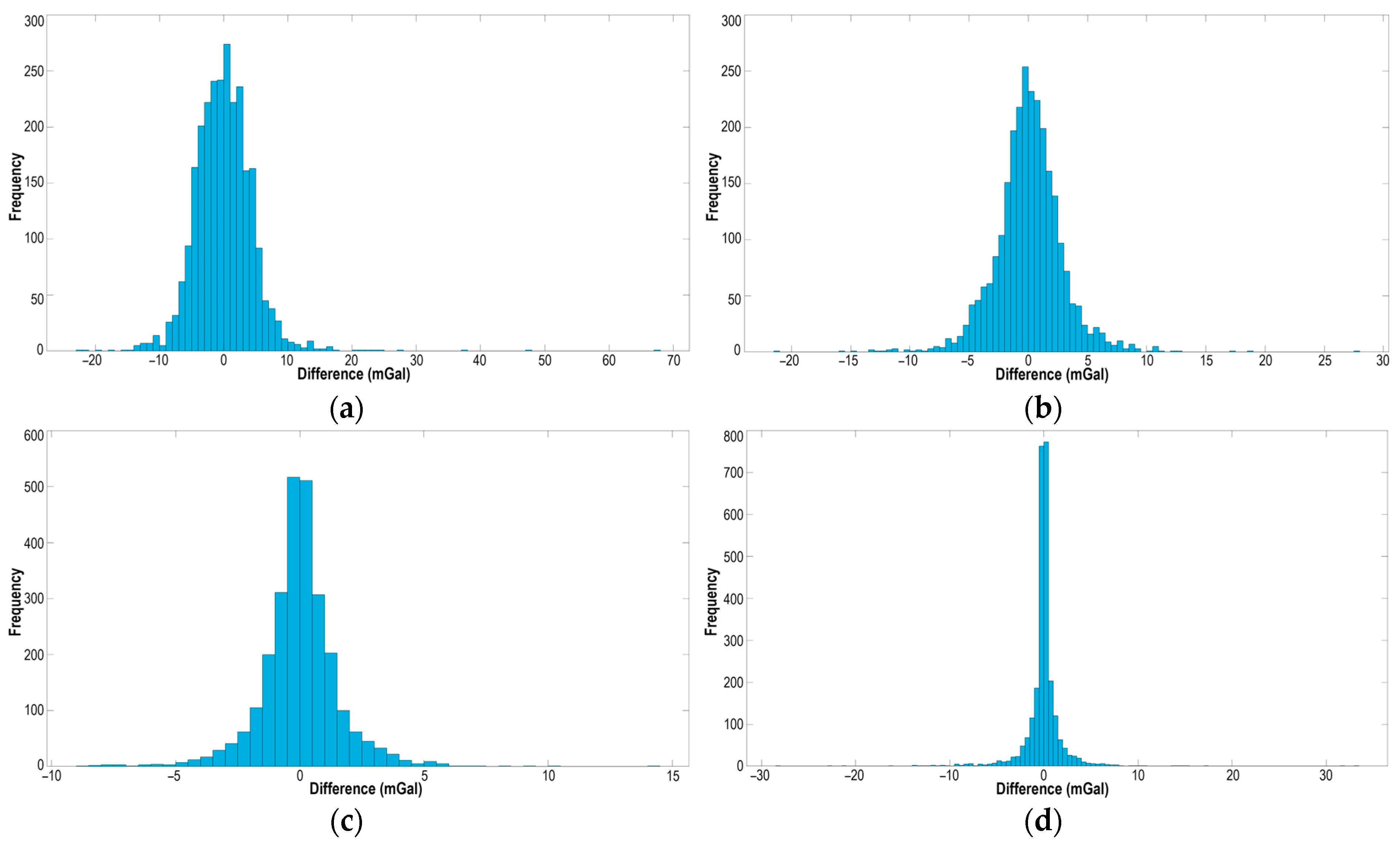
It is important to note that, although the Exponential GPR model predicts a higher percentage of values with errors below 1 mGal compared to the Kriging interpolation method, the error distribution in Exponential GPR exhibits more pronounced outliers (±30 mGal). This is confirmed by the histograms (Figure 5d), where individual values with significant deviations from zero are observed, indicating a higher amplitude of extreme errors compared to Kriging (Figure 5c). The Kriging method demonstrates a smoother error, distribution with fewer points exceeding the ±10 mGal range, indicating its greater robustness to outliers. Analyzing the spatial distribution of points with errors exceeding 3 mGal predicted by Exponential GPR, a clear pattern in the location of outliers can be observed. The majority of these errors are concentrated in the eastern and southeastern parts of the study area, which are characterized by significant elevation changes and the presence of mountain ranges (Figure 2b).

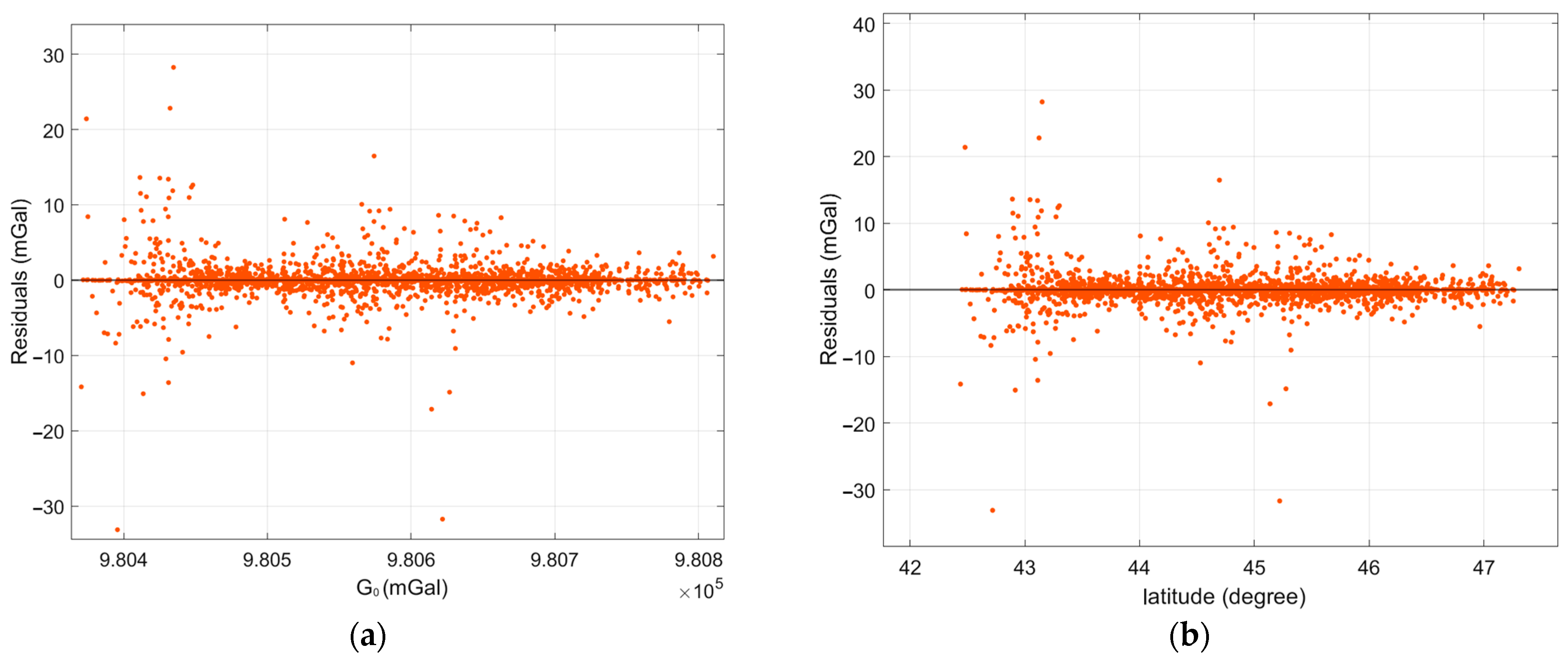
Figure 6 presents the differences between the actual and predicted simple Bouguer anomaly values as functions of normal gravity (G₀), latitude, longitude, elevation (H), and terrain correction (TC). An analysis of the presented graphs reveals that the largest discrepancies are observed in mountainous regions. Geographically, the errors correlate with areas of high terrain correction values, greater elevations, and specific latitude and longitude ranges, which correspond to the locations of mountain ranges (Figure 2b).

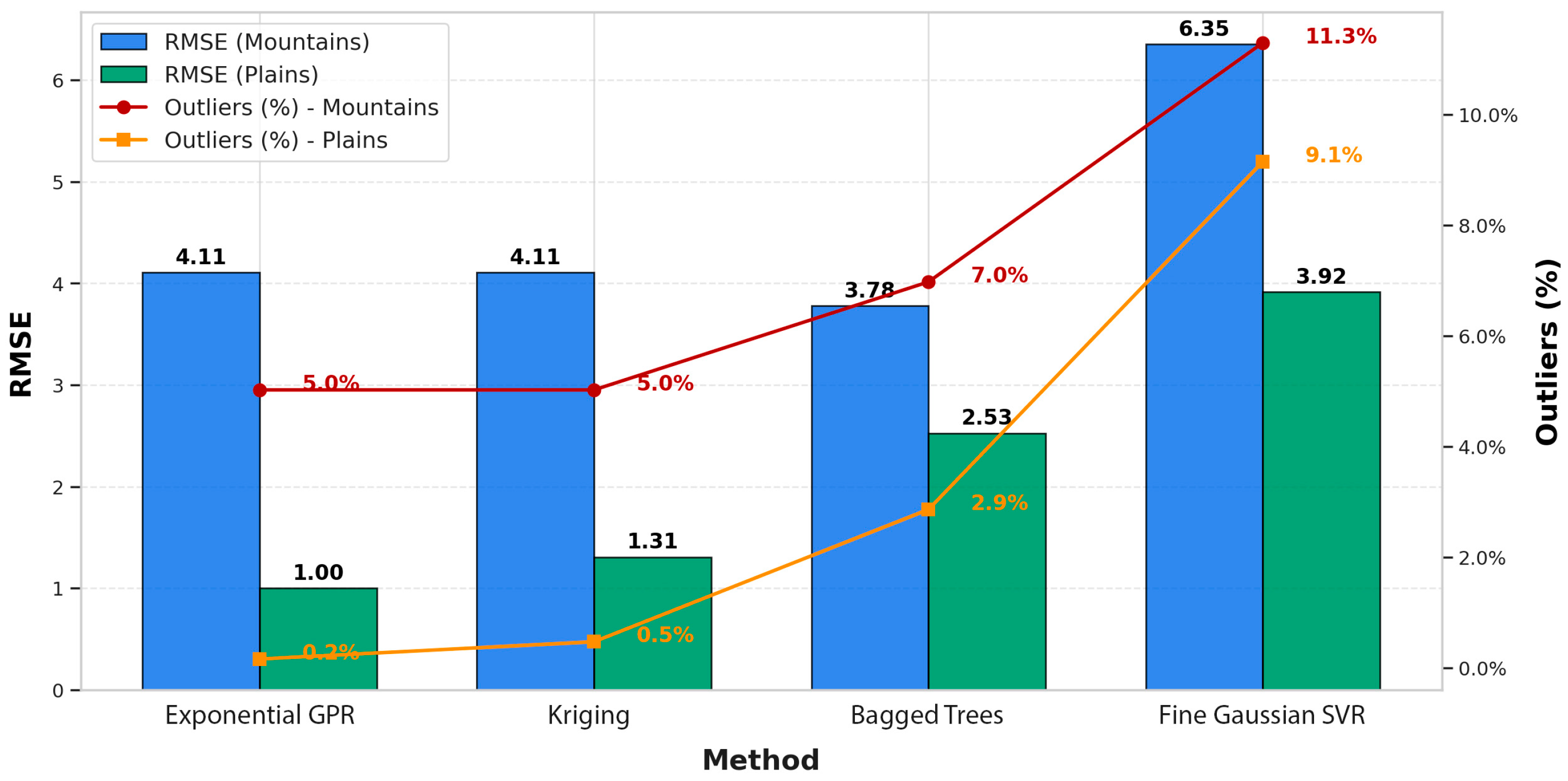
Based on the identified pattern, the initial dataset was divided into two subsets: lowland and mountainous. Figure 7 presents the accuracy assessment of the simple Bouguer anomaly prediction methods under mountainous and lowland conditions. An analysis of RMSE values in mountainous regions revealed that machine learning methods experience significant decreases in accuracy compared to in lowland areas, as indicated by higher errors and increased numbers of outliers. The highest RMSE value was observed for Fine Gaussian SVR (6.35), suggesting its low robustness to complex terrain. In contrast, Exponential GPR (4.11) and Kriging (4.11) demonstrated relatively more stable performances. The Bagged Trees algorithm achieved the lowest RMSE value (3.78) in mountainous regions; however, it also exhibited a notable increase in outliers (7.0%).

4. Discussion

The performance and generalizability of each model was influenced by several factors, particularly in mountainous regions. While some of these reflect inherent limitations in data availability and methodological setup, others reveal important behavioral characteristics of the models themselves.

First, we employed simple Bouguer anomalies, which do not include terrain corrections, due to the incomplete availability of terrain correction data across a significant portion of the study area. An additional analysis of the relationship between prediction errors and terrain corrections, presented in Figure 6e, shows that errors systematically increase with higher terrain correction values. In regions where terrain corrections were absent (assigned a value of zero), prediction errors remained relatively low and stable. However, in areas where terrain corrections were substantial—typically corresponding to mountainous regions—larger deviations and higher concentrations of outliers were observed, particularly for the Exponential GPR model.

Second, the same grid spacing was applied across the entire study area, regardless of terrain complexity. Consequently, the data density in mountainous areas was relatively low compared to in flat regions, leading to reduced model training efficiency and increased interpolation errors in areas with rapid changes in elevation.

Third, with regards to algorithmic sensitivity, although all tested machine learning models demonstrated the ability to predict gravity anomalies to varying degrees of accuracy, notable differences in performance were observed. The Fine Gaussian SVR and Bagged Trees models showed comparatively lower predictive capabilities across both lowland and mountainous regions. This behavior can be attributed to inherent algorithmic characteristics: SVR models are known to be highly sensitive to data noise and require careful tuning of kernel parameters, which makes them less robust in complex and heterogeneous datasets. Bagged Trees, while effective in reducing variance through ensemble learning, are primarily suited for discrete classification tasks and may struggle to accurately model continuous and subtle variations typical of geophysical fields such as gravity anomalies.

In contrast, Exponential GPR demonstrated significantly better predictive performance. This can be explained by the algorithm’s intrinsic strengths: GPR is a non-parametric, probabilistic model capable of capturing complex nonlinear relationships, while simultaneously providing uncertainty estimates for each prediction. Its ability to flexibly model spatial variability made it particularly effective in smooth, continuous regions, where gravity changes gradually. However, GPR’s performance showed sensitivity to data sparsity and abrupt topographic variations, as indicated by the presence of a few extreme outliers in mountainous areas. These outliers are consistent with the Bayesian nature of GPR, which, under conditions of limited and irregularly distributed training data, can lead to amplified prediction uncertainties. In contrast, Kriging, by design, constrains predictions based on spatial autocorrelation, leading to smoother, more conservative interpolation results even under challenging conditions. Therefore, while Exponential GPR generally outperformed other methods in terms of predictive accuracy, its flexibility also made it more vulnerable to producing rare but higher-magnitude deviations in complex terrains.

While some limitations affected model performance in specific regions, the overall results confirm the potential of ML approaches for gravity anomaly prediction under realistic data conditions. In particular, the Exponential GPR model achieved the best performance when predicting simple Bouguer anomalies: only 7.9% of the points exhibited errors exceeding 3 mGal, while 72.9% of the predictions showed errors below 1 mGal. These results highlight the strong predictive capability of the Exponential GPR model in gravity data modeling tasks.

Future research will focus on several key directions aimed at improving model accuracy. First, the capability of machine learning models to predict gravity anomalies will be examined under conditions where the influence of topography is minimized or eliminated. To this end, complete Bouguer anomalies, which incorporate terrain corrections, will be computed. This will help determine whether the reduced performance of the Exponential GPR model in mountainous areas is due to the absence of topographic correction when using simple Bouguer anomalies.

Additionally, future research may explore a wider range of modeling approaches to further improve predictive performance. In particular, deep learning (DL) methods, such as convolutional neural networks (CNNs) and recurrent neural networks (RNNs), will be considered as promising tools for capturing complex spatial patterns. These approaches, used in complement to the current methods, could contribute to more robust and adaptable gravity anomaly prediction models.

5. Conclusions

This study presents a comparative analysis of the traditional Kriging interpolation method and modern machine learning algorithms, namely Gaussian Process Regression (Squared Exponential, Matern 5/2, Exponential, and Rational Quadratic), Ensembles of Trees (Bagged Trees and Boosted Trees) and Support Vector Regression (Linear, Quadratic, Cubic, Fine Gaussian, Medium Gaussian, and Coarse Gaussian) for predicting simple Bouguer anomaly values. The initial dataset was divided into two subsets, a learning set and an independent test set, incorporating parameters such as simple Bouguer anomaly, latitude, longitude, elevation, normal gravity. The machine learning models for gravity data prediction were trained in the MATLAB^® environment (version R2024a). Among the machine learning methods examined in the experiments, Exponential GPR demonstrated the best predictive performance. The Kriging method also produced highly accurate results, confirming its effectiveness in interpolation tasks. In contrast, the Fine Gaussian SVR algorithm exhibited the lowest predictive accuracy among the evaluated machine learning models.

This study has demonstrated that machine learning algorithms can be effectively applied to gravity data prediction tasks. However, the selection of a specific algorithm should be based on its predictive performance across different conditions.