
Machine-Learning Models and Global Sensitivity Analyses to Explicitly Estimate Groundwater Presence Validated by Observed Dataset at K-NET in Japan


Abstract
1. Introduction
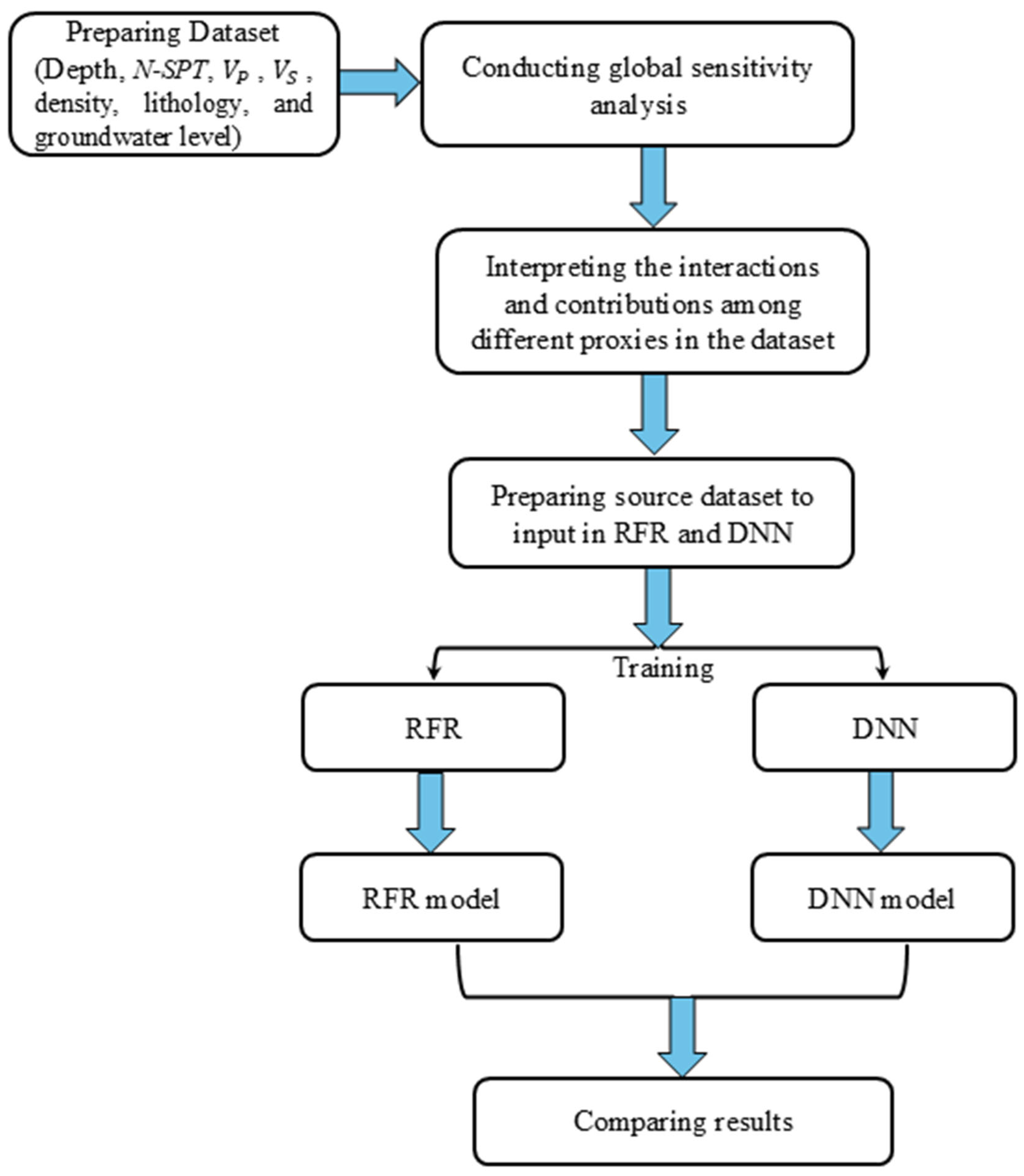
2. Methodology
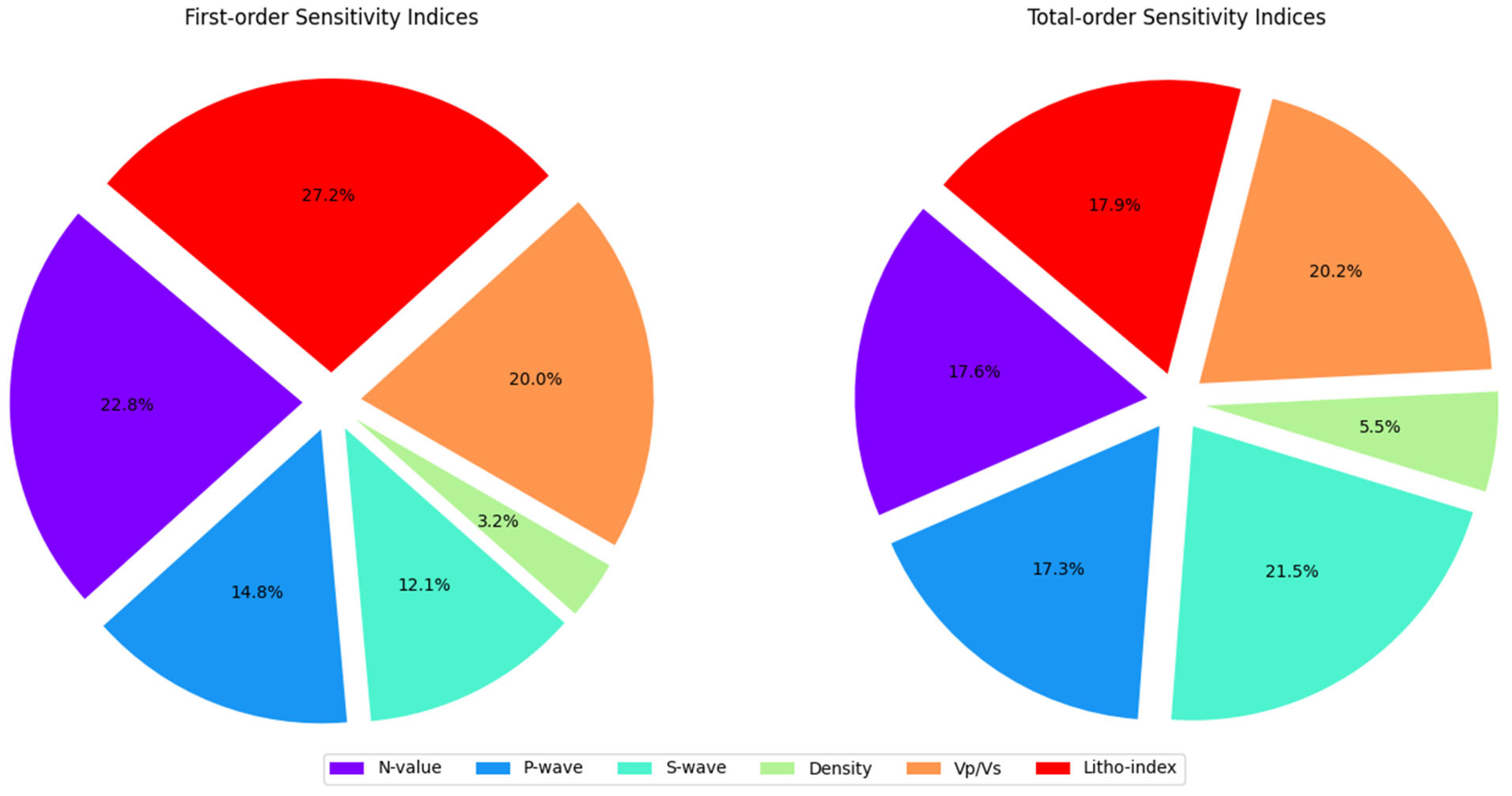
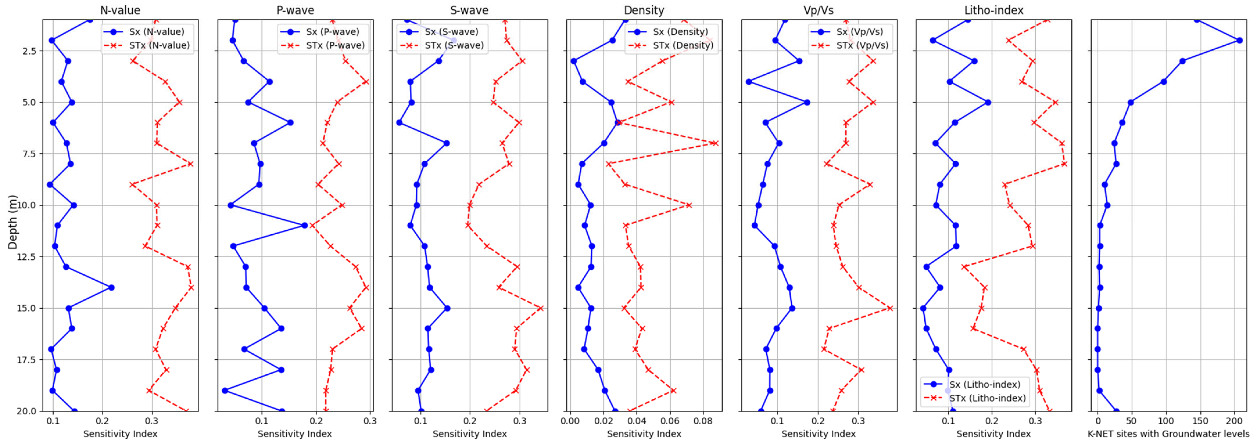
2.1. Global Sensitivity Analyses
2.2. DNN
2.3. RFR
- The training datasets comprise a set of samples (i.e., K-NET sites), and each sample, consequently, contains a set of features (i.e., Depth, N-SPT, , , , , Poisson’s ratio, P- and S-wave impedance contrasts, , and lithology). At each decision tree in the RFR, the training datasets are sampled as bootstrap and out-of-bag () datasets of approximate ratio two-to-one, respectively. The bootstrap samples are generated to train the model, whereas out-of-bag () samples are used to evaluate the model by averaging the predictions all over the decision trees. The evaluation using is an important step for providing the generalization applicability to the resulting RFR model.
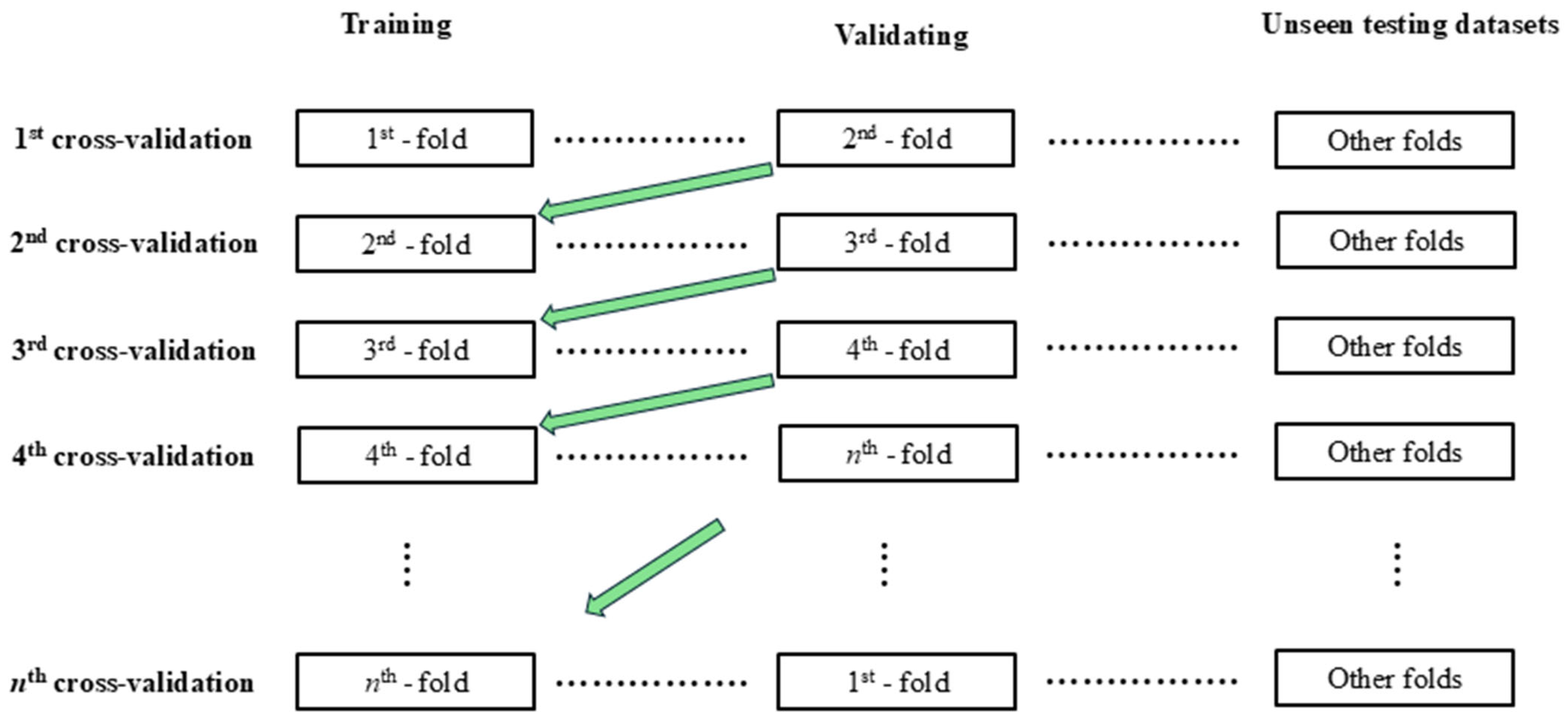
- The k-fold cross-validation procedure is applied. It is acquired from the Scikit-learn library in the Python framework. A thirteen-fold cross-validation approach is adopted.
- The hyperparameters are tuned utilizing grid search capability in the Scikit-learn library. These hyperparameters are the number of decision trees, the maximum depth of these trees, the minimum splits of bootstrap samples, and the minimum sample leaves for these decision trees. This step consumes a long analysis period to yield the highest-performing RFR model.
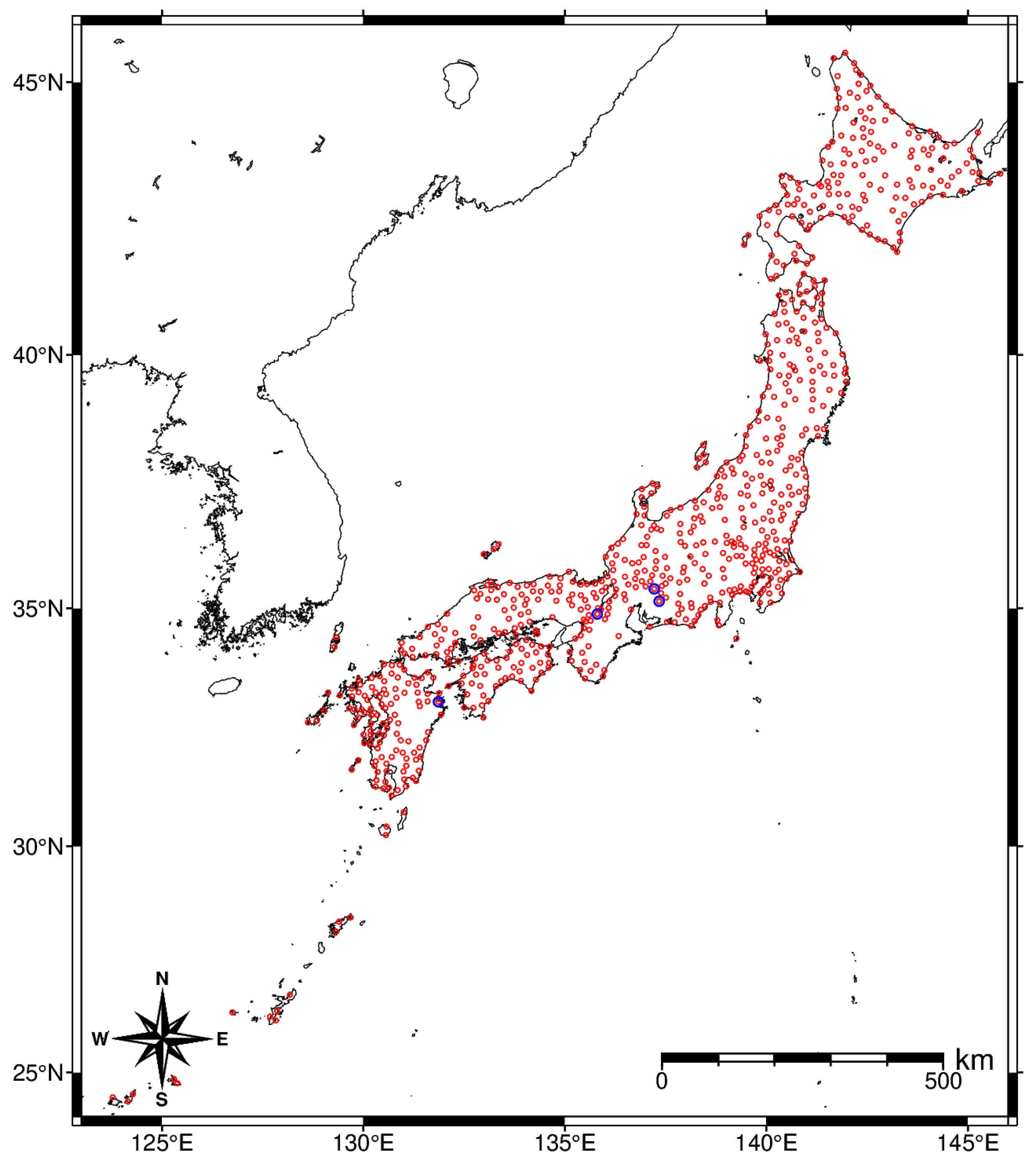
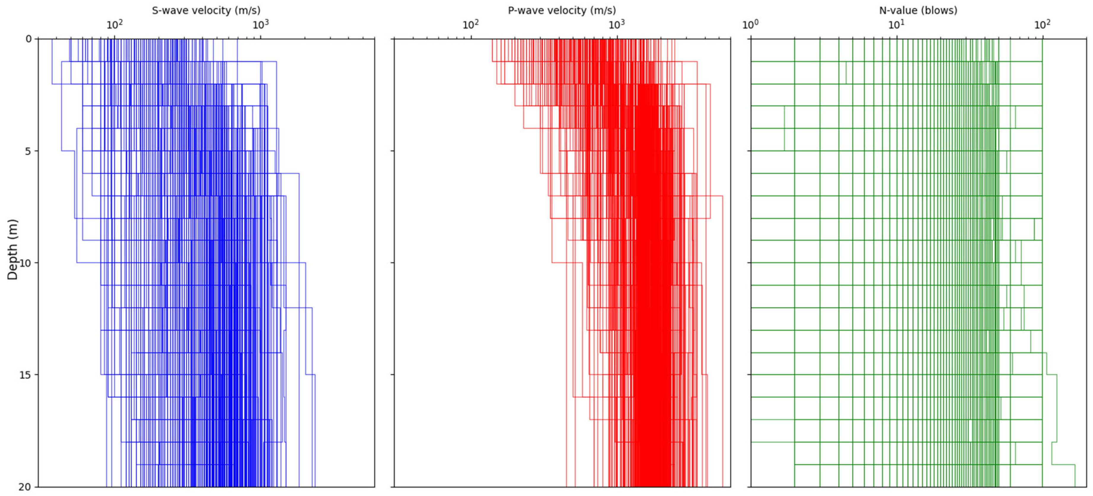
3. Data
4. Results and Discussion
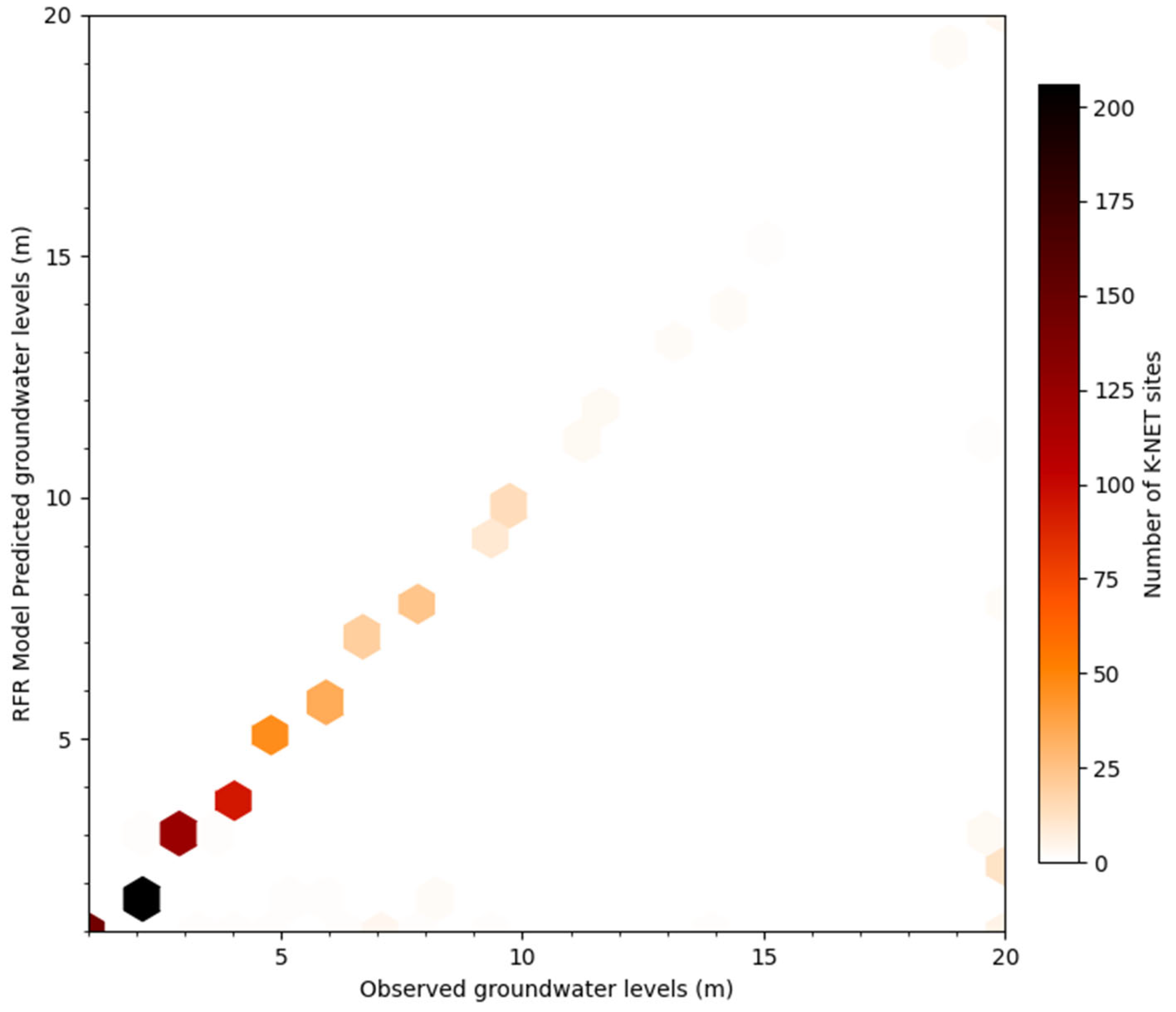
4.1. Performance of the RFR Model
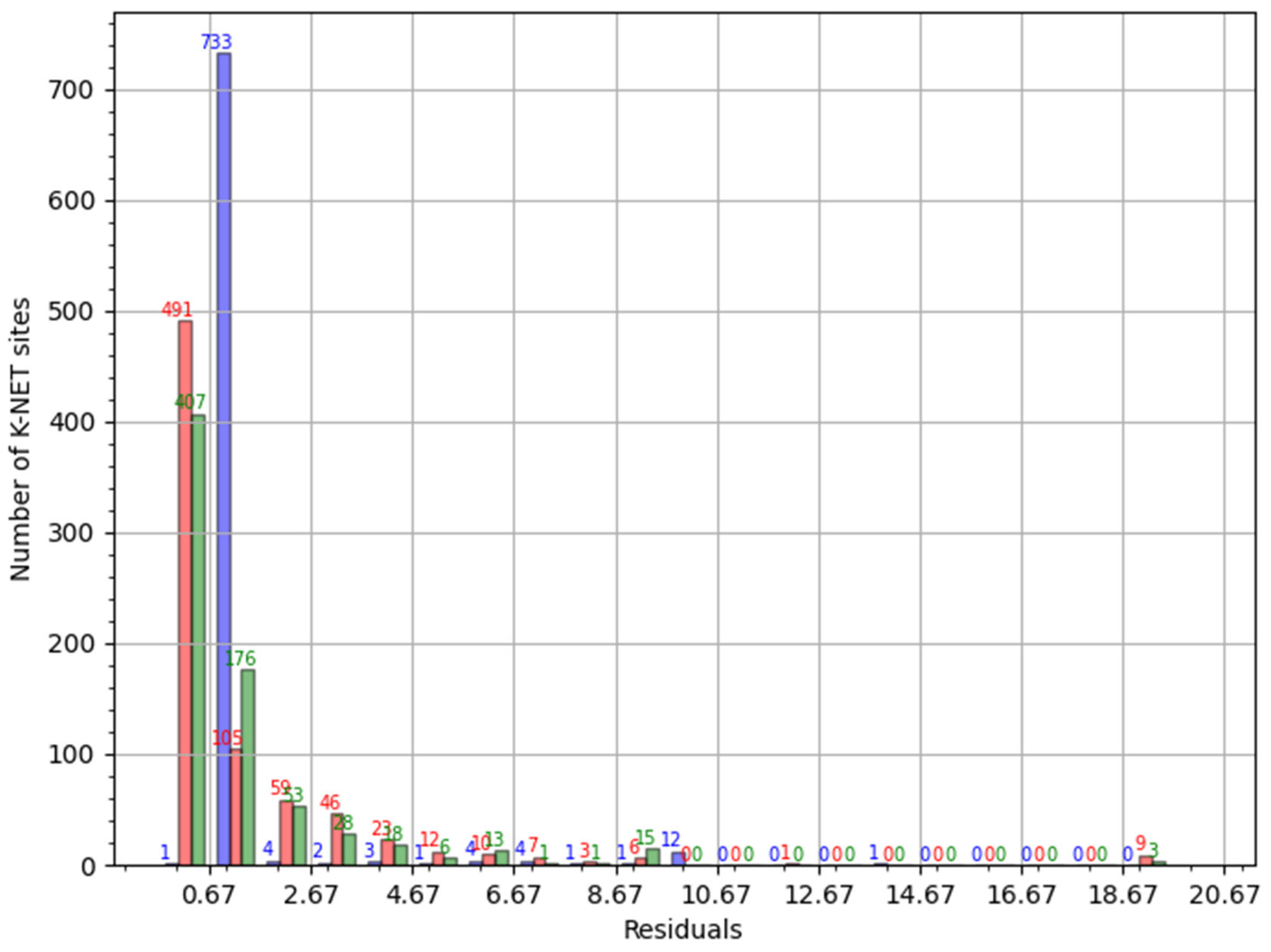
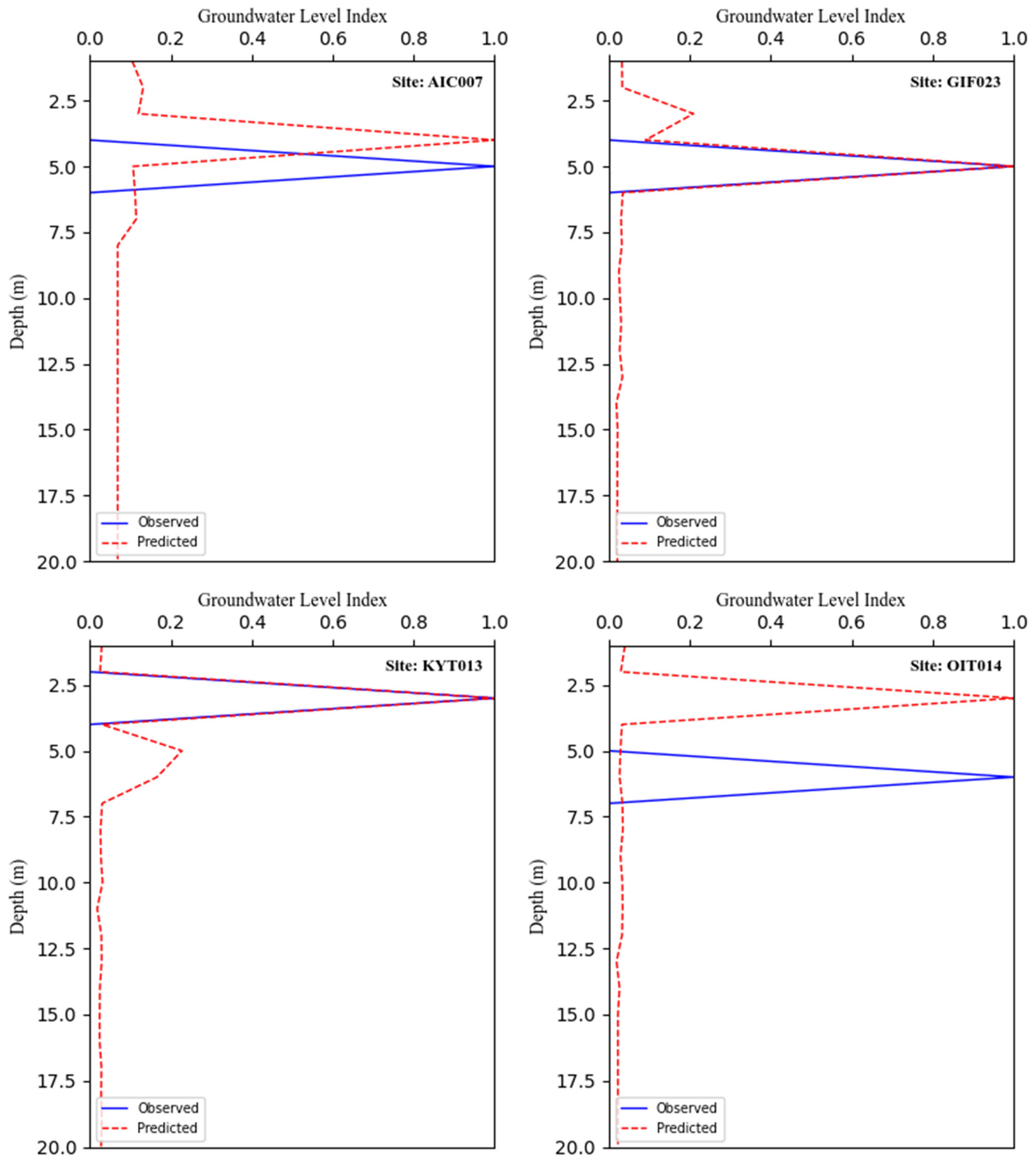
4.2. Validating the RFR Model
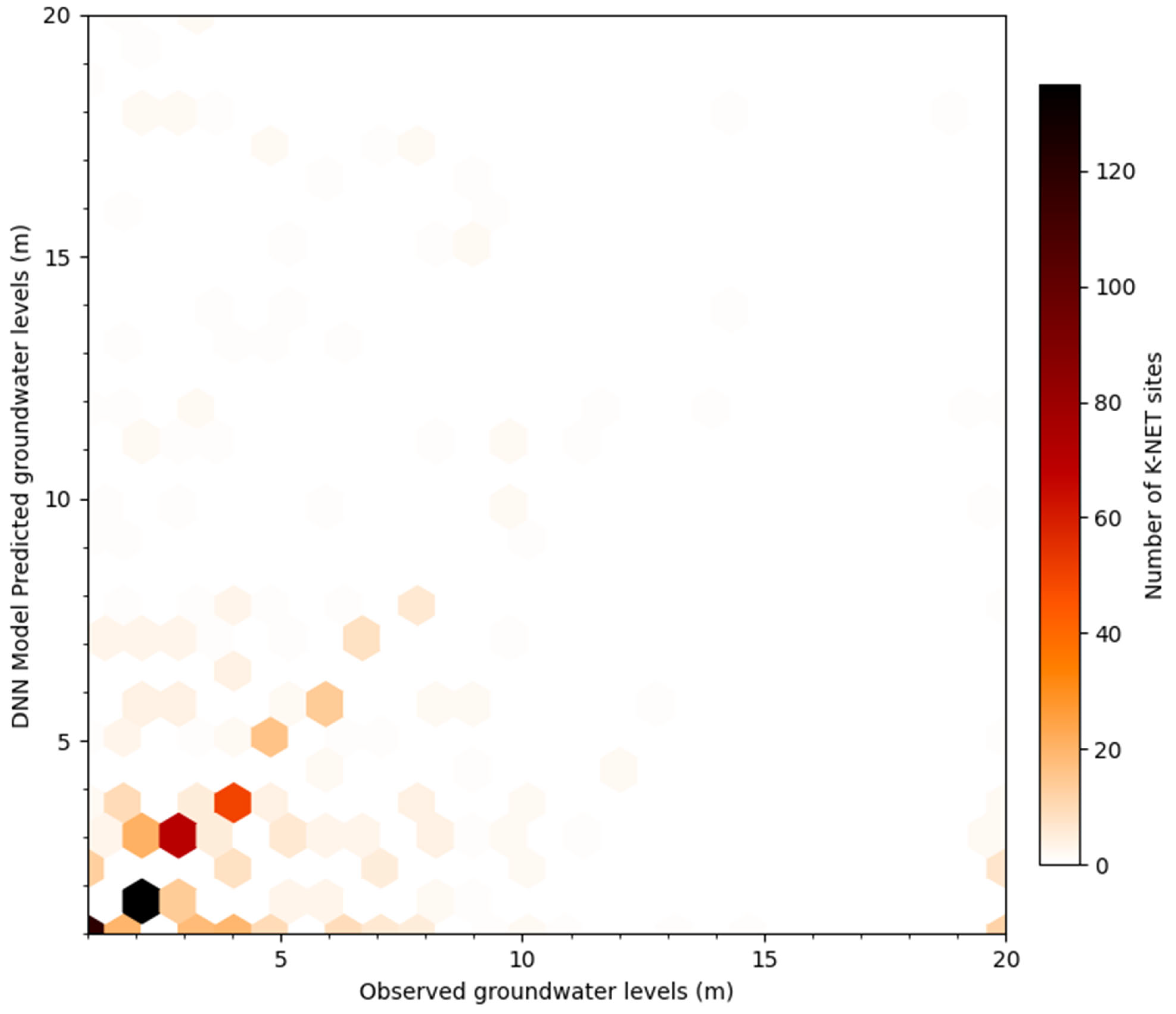
4.3. Performance of the DNN Model
4.4. Global Sensitivity Analyses
4.5. Prospecting Applicability
5. Conclusions
Funding
Data Availability Statement
Acknowledgments
Conflicts of Interest
References
- Satoh, Y.; Yoshimura, K.; Pokhrel, Y.; Kim, H.; Shiogama, H.; Yokohata, T.; Hanasaki, N.; Wada, Y.; Burek, P.; Byers, E.; et al. The timing of unprecedented hydrological drought under climate change. Nat. Commun. 2022, 13, 3287. [Google Scholar] [CrossRef] [PubMed]
- Wanders, N.; Wada, Y.; Van Lanen, H.A.J. Global hydrological droughts in the 21st century under a changing hydrological regime. Earth Syst. Dyn. 2015, 6, 61–81. [Google Scholar] [CrossRef]
- Hari, V.; Rakovec, O.; Markonis, Y.; Hanel, M.; Kumar, R. Increased future occurrences of the exceptional 2018–2019 Central European drought under global warming. Sci. Rep. 2020, 10, 12207. [Google Scholar] [CrossRef]
- Bertoni, C.; Lofi, J.; Micallef, A.; Moe, H. Reflection Methods in Offshore Groundwater Research. Geosciences 2020, 10, 299. [Google Scholar] [CrossRef]
- Thabet, M. Applicability of a proposed groundwater level determination approach for the K-NET in Japan. Near Surf. Geophys. 2021, 19, 447–463. [Google Scholar] [CrossRef]
- Biot, M.A. Theory of propagation of elastic waves in fluid-saturated porous solid. Part I: Low frequency range. J. Acoust. Soc. Am. 1956, 28, 168–178. [Google Scholar] [CrossRef]
- Biot, M.A. Theory of propagation of elastic waves in fluid saturated porous solid. Part II: Higher frequency range. J. Acoust. Soc. Am. 1956, 28, 179–191. [Google Scholar] [CrossRef]
- Grelle, G.; Guadagno, F.M. Seismic refraction methodology for groundwater level determination: “Water seismic index”. J. Appl. Geophys. 2009, 68, 301–320. [Google Scholar] [CrossRef]
- Dvorkin, J. Yet another Vs equation. Geophysics 2008, 73, E35–E39. [Google Scholar] [CrossRef]
- Uyanık, O. The porosity of saturated shallow sediments from seismic compressional and shear wave velocities. J. Appl. Geophys. 2011, 73, 16–24. [Google Scholar] [CrossRef]
- Konstantaki, L.A.; Carpentier, S.F.A.; Garofalo, F.; Bergamo, P.; Socco, L.V. Determining hydrological and soil mechanical parameters from multichannel surface-wave analysis across the Alpine Fault at Inchbonnie, New Zealand. Near Surf. Geophys. 2013, 11, 435–448. [Google Scholar] [CrossRef]
- Bachrach, R.; Nur, A. High-resolution shallow-seismic experiments in sand, part I: Water table, fluid flow, and saturation. Geophysics 1998, 63, 1225–1233. [Google Scholar] [CrossRef]
- Zelt, A.C.; Azaria, A.; Levander, A. 3D seismic refraction traveltime tomography at a groundwater contamination site. Geophysics 2006, 58, 1314–1323. [Google Scholar] [CrossRef]
- Nagashima, F.; Kawase, H. The relationship between Vs, Vp, density and depth based on PS-logging data at K-NET and KiK-net sites. Geophys. J. Int. 2021, 225, 1467–1491. [Google Scholar] [CrossRef]
- Adam, L.; Batzle, M.; Brevik, I. Gassmann’s fluid substitution and shear modulus variability in carbonates at laboratory seismic and ultrasonic frequencies. Geophysics 2006, 71, F173–F183. [Google Scholar] [CrossRef]
- Ghasemzadeh, H.; Abounouri, A.A. Effect of subsurface hydrological properties on velocity and attenuation of compressional and shear wave in fluid-saturated viscoelastic porous media. J. Hydrol. 2012, 460–461, 110–116. [Google Scholar] [CrossRef]
- NEID. K-NET, KiK-net, National Research Institute for Earth Science and Disaster Resilience. 2019. Available online: https://www.kyoshin.bosai.go.jp (accessed on 17 December 2024).
- Herman, J.D.; Usher, W. SALib: Sensitivity Analysis Library in Python. J. Open Source Softw. 2017, 2, 97. [Google Scholar] [CrossRef]
- Saltelli, A.; Tarantola, S.; Chan, K. A Quantitative Model-Independent Method for Global Sensitivity Analysis of Model Output. Technometrics 1999, 41, 39–56. [Google Scholar] [CrossRef]
- Saltelli, A. Making best use of model evaluations to compute sensitivity indices. Comput. Phys. Commun. 2002, 145, 280–297. [Google Scholar] [CrossRef]
- Sobol, I.M. Global sensitivity indices for nonlinear mathematical models and their Monte Carlo estimates. Math. Comput. Simul. 2001, 55, 271–280. [Google Scholar] [CrossRef]
- Lovatti, B.P.O.; Nascimento, M.H.C.; Neto, Á.C.; Castro, E.V.R.; Filgueiras, P.R. Use of Random forest in the identification of important variables. Microchem. J. 2019, 145, 1129–1134. [Google Scholar] [CrossRef]
- Khan, I.; Ayaz, M. Sensitivity analysis-driven machine learning approach for groundwater quality prediction: Insights from integrating ENTROPY and CRITIC methods. Groundw. Sustain. Dev. 2024, 26, 101309. [Google Scholar] [CrossRef]
- Hayashi, K.; Suzuki, T.; Inazaki, T.; Konishi, C.; Suzuki, H.; Matsuyama, H. Estimating S-wave velocity profiles from horizontal-to-vertical spectral ratios based on deep learning. Soils Found. 2024, 64, 101525. [Google Scholar] [CrossRef]
- Pan, D.; Miura, H.; Kwan, C. Transfer learning model for estimating site amplification factors from limited microtremor H/V spectral ratios. Geophys. J. Int. 2024, 237, 622–635. [Google Scholar] [CrossRef]
- Zhu, J.; Li, S.; Song, J. Data-knowledge driven hybrid deep learning for earthquake early warning. Earth Space Sci. 2024, 11, e2023EA003363. [Google Scholar] [CrossRef]
- Abadi, M.; Barham, P.; Chen, J.; Chen, Z.; Davis, A.; Dean, J.; Devin, M.; Ghemawat, S.; Irving, G.; Isard, M.; et al. TensorFlow: A system for large-scale machine learning. In Proceedings of the 12th USENIX Symposium on Operating Systems Design and Implementation, Savannah, GA, USA, 2–4 November 2016; (OSDI ’16). USENIX Association: Berkeley, CA, USA, 2016; pp. 265–283. Available online: https://www.tensorflow.org (accessed on 1 January 2025).
- Arthur, D.; Vassilvitskii, S. K-means++the advantages of careful seeding. In Proceedings of the 18th Annual ACM-SIAM Symposium on Discrete Algorithms, New Orleans, LA, USA, 7–9 January 2007; pp. 1027–1035. [Google Scholar]
- Chen, R.; Zhang, P.; Wu, H.; Wang, Z.T.; Zhong, Z.Q. Prediction of shield tunneling-induced ground settlement using machine learning techniques. Front. Struct. Civ. Eng. 2019, 13, 1363–1378. [Google Scholar] [CrossRef]
- Boore, D.M. Estimating VS (30) (or NEHRP site classes) from shallow velocity models (depths < 30 m). Bull. Seismol. Soc. Am. 2004, 94, 591–597. [Google Scholar] [CrossRef]
- FEMA P-2082-1; (National Earthquake Hazards Reduction Program) Recommended Seismic Provisions for New Buildings and Other Structures. National Institute of Building Sciences: Washington, DC, USA, 2020; Volume I, Part 1 Provisions and Part 2 Commentary. Available online: https://www.fema.gov/sites/default/files/2020-10/fema_2020-nehrp-provisions_part-1-and-part-2.pdf (accessed on 1 January 2025).
- Jia, R.; Lv, Y.; Wang, G.; Carranza, E.; Chen, Y.; Wei, C.; Zhang, Z. A stacking methodology of machine learning for 3D geological modeling with geological-geophysical datasets, Laochang Sn camp, Gejiu (China). Comput. Geosci. 2021, 151, 104754. [Google Scholar] [CrossRef]
- Thibaut, R.; Laloy, E.; Hermans, T. A new framework for experimental design using Bayesian Evidential Learning: The case of wellhead protection area. J. Hydrol. 2021, 603, 126903. [Google Scholar] [CrossRef]
- Breiman, L. Random Forests. Mach. Learn. 2001, 45, 5–32. [Google Scholar] [CrossRef]
- Hastie, T.; Tibshirani, R.; Friedman, J. Random Forests. In The Elements of Statistical Learning; Springer: New York, NY, USA, 2009. [Google Scholar] [CrossRef]
- Watson, D.B.; Doll, W.E.; Jeffrey Gamey, T.; Sheehan, J.R.; Jardine, P.M. Plume and lithologic profiling with surface resistivity and seismic tomography. Ground Water 2005, 43, 169–177. [Google Scholar] [CrossRef] [PubMed]
- Danneels, G.; Bourdeau, C.; Torgoev, I.; Havenith, H.B. Geophysical investigation and dynamic modelling of unstable slopes: Case-study of Kainama (Kyrgyzstan). Geophys. J. Int. 2008, 175, 17–34. [Google Scholar] [CrossRef]
- Thabet, M.; Nagashima, F.; Kawase, H. A computational approach for bedrock regressions with diffuse field concept beneath the Japan Islands. Soil Dyn. Earthquake Eng. 2024, 177, 108429. [Google Scholar] [CrossRef]
- Thabet, M.; Omar, K. Subsurface velocity structures at the Egyptian seismological network stations retrieved by diffuse field assumption for Earthquakes. Eng. Geol. 2024, 338, 107626. [Google Scholar] [CrossRef]
- Gardner, G.H.F.; Gardner, L.W.; Gregory, A.R. Formation velocity and density—The diagnostic basics for stratigraphic traps. Geophysics 1974, 39, 770–780. [Google Scholar] [CrossRef]
- Munirwansyah, M.; Fulazzaky, M.A.; Yunita, H.; Munirwan, R.P.; Jonbi, J.; Sumeru, K. A new empirical equation of shear wave velocity to predict the different peak surface accelerations for Jakarta city. Geod. Geodyn. 2020, 11, 455–467. [Google Scholar] [CrossRef]
- Wang, Z.; Cai, Y.; Liu, D.; Lu, J.; Qiu, F.; Sun, F.; Hu, J.; Li, Z. Characterization of natural fracture development in coal reservoirs using logging machine learning inversion, well test data and simulated geostress analyses. Eng. Geol. 2024, 341, 107696. [Google Scholar] [CrossRef]


| Index | Definition |
|---|---|
| 1 | surface soil |
| 2 | fill soil |
| 3 | gravel |
| 4 | gravelly soil |
| 5 | sand |
| 6 | sandy soil |
| 7 | silt |
| 8 | clay |
| 9 | organic soil |
| 10 | volcanic ash clay |
| 11 | peat |
| 12 | rock |
| Depth (m) | N-SPT | (m/s) | (m/s) | (m/s) | (g/cm3) | LI 2 | Poisson’s Ratio | ICP 1 | ICS 1 | GLI 2 | |
|---|---|---|---|---|---|---|---|---|---|---|---|
| 1 | 10 | 240 | 110 | 318 | 1.61 | 1 | 2.18 | 0.367 | −0.013 | −0.013 | 0 |
| 2 | 24 | 240 | 110 | 318 | 1.57 | 1 | 2.18 | 0.367 | 0.724 | 0.423 | 0 |
| 3 | 20 | 1550 | 280 | 318 | 1.52 | 1 | 5.54 | 0.483 | 0.041 | 0.041 | 1 |
| 4 | 34 | 1550 | 280 | 318 | 1.65 | 1 | 5.54 | 0.483 | 0.015 | 0.015 | 0 |
| 5 | 34 | 1550 | 280 | 318 | 1.70 | 1 | 5.54 | 0.483 | 0.020 | 0.020 | 0 |
| 6 | 34 | 1550 | 280 | 318 | 1.77 | 1 | 5.54 | 0.483 | 0.046 | 0.046 | 0 |
| 7 | 25 | 1550 | 280 | 318 | 1.94 | 1 | 5.54 | 0.483 | −0.037 | −0.037 | 0 |
| 8 | 24 | 1550 | 280 | 318 | 1.80 | 8 | 5.54 | 0.483 | 0.014 | 0.014 | 0 |
| 9 | 23 | 1550 | 280 | 318 | 1.85 | 7 | 5.54 | 0.483 | 0.026 | 0.026 | 0 |
| 10 | 28 | 1550 | 280 | 318 | 1.95 | 7 | 5.54 | 0.483 | 0.191 | 0.205 | 0 |
| 11 | 99 | 2260 | 420 | 318 | 1.97 | 5 | 5.38 | 0.482 | 0.010 | 0.010 | 0 |
| 12 | 99 | 2260 | 420 | 318 | 2.01 | 3 | 5.38 | 0.482 | 0.015 | 0.015 | 0 |
| 13 | 99 | 2260 | 420 | 318 | 2.07 | 3 | 5.38 | 0.482 | 0.012 | 0.012 | 0 |
| 14 | 99 | 2260 | 420 | 318 | 2.12 | 4 | 5.38 | 0.482 | −0.014 | −0.014 | 0 |
| 15 | 99 | 2260 | 420 | 318 | 2.06 | 4 | 5.38 | 0.482 | −0.007 | −0.007 | 0 |
| 16 | 99 | 2260 | 420 | 318 | 2.03 | 4 | 5.38 | 0.482 | −0.012 | −0.012 | 0 |
| 17 | 99 | 2260 | 420 | 318 | 1.98 | 3 | 5.38 | 0.482 | 0.003 | 0.003 | 0 |
| 18 | 99 | 2260 | 420 | 318 | 1.99 | 3 | 5.38 | 0.482 | 0.017 | 0.017 | 0 |
| 19 | 99 | 2260 | 420 | 318 | 2.06 | 3 | 5.38 | 0.482 | −0.010 | −0.010 | 0 |
| 20 | 99 | 2260 | 420 | 318 | 2.02 | 3 | 5.38 | 0.482 | 0.000 | 0.000 | 0 |
| Validation Approaches | No. of K-NET Sites When Residual (r) | Failed Groundwater Detection at K-NET Sites | |||
|---|---|---|---|---|---|
| 0.1 < r < 1.0 (Overestimate) | r ≈ 1.0 (Match) | 1.0 < r < 10.0 (Underestimate) | |||
| k-fold cross-validation | 1 | 733 | 33 | 5 | |
| Training %–Validating % (772 K-NET sites) | 90–10% | 16 | 686 | 63 | 7 |
| 70–30% | 50 | 572 | 143 | 7 | |
| 50–50% | 121 | 462 | 176 | 13 | |
| 30–70% | 161 | 387 | 216 | 8 | |
| 20–80% | 171 | 310 | 277 | 29 | |
| 10–90% | 164 | 237 | 357 | 14 | |
| Validation Approaches | No. of K-NET Sites When Residual (r) | Failed Groundwater Detection at K-NET Sites | |||
|---|---|---|---|---|---|
| 0.1 < r < 1.0 (Overestimate) | r ≈ 1.0 (Match) | 1.0 < r < 10.0 (Underestimate) | |||
| k-fold cross-validation | 135 | 470 | 155 | 12 | |
| Training %–Validating % (772 K-NET sites) | 90–10% | 198 | 317 | 245 | 12 |
| 70–30% | 171 | 287 | 304 | 10 | |
| 50–50% | 302 | 281 | 178 | 11 | |
| 30–70% | 311 | 256 | 194 | 11 | |
| 20–80% | 306 | 243 | 217 | 6 | |
| 10–90% | 353 | 218 | 197 | 4 | |
Disclaimer/Publisher’s Note: The statements, opinions and data contained in all publications are solely those of the individual author(s) and contributor(s) and not of MDPI and/or the editor(s). MDPI and/or the editor(s) disclaim responsibility for any injury to people or property resulting from any ideas, methods, instructions or products referred to in the content. |
© 2025 by the author. Licensee MDPI, Basel, Switzerland. This article is an open access article distributed under the terms and conditions of the Creative Commons Attribution (CC BY) license (https://creativecommons.org/licenses/by/4.0/).
Share and Cite
Thabet, M. Machine-Learning Models and Global Sensitivity Analyses to Explicitly Estimate Groundwater Presence Validated by Observed Dataset at K-NET in Japan. Geosciences 2025, 15, 126. https://doi.org/10.3390/geosciences15040126
Thabet M. Machine-Learning Models and Global Sensitivity Analyses to Explicitly Estimate Groundwater Presence Validated by Observed Dataset at K-NET in Japan. Geosciences. 2025; 15(4):126. https://doi.org/10.3390/geosciences15040126
Chicago/Turabian StyleThabet, Mostafa. 2025. "Machine-Learning Models and Global Sensitivity Analyses to Explicitly Estimate Groundwater Presence Validated by Observed Dataset at K-NET in Japan" Geosciences 15, no. 4: 126. https://doi.org/10.3390/geosciences15040126
APA StyleThabet, M. (2025). Machine-Learning Models and Global Sensitivity Analyses to Explicitly Estimate Groundwater Presence Validated by Observed Dataset at K-NET in Japan. Geosciences, 15(4), 126. https://doi.org/10.3390/geosciences15040126