Study on Post-Stack Signal Denoising for Long-Offset Transient Electromagnetic Data Based on Combined Windowed Interpolation and Singular Spectrum Analysis

Abstract

The long-offset transient electromagnetic (LOTEM) method, as a widely applied electromagnetic exploration technique, plays a significant role in mineral resource exploration, hydraulic fracturing monitoring, and fluid identification in oil and gas reservoirs. However, due to external interference, the signals acquired by this method often contain substantial noise, which severely affects the reliability of subsequent inversion and interpretation. Therefore, denoising is a critical issue in LOTEM data processing. To address this problem, this paper proposes a denoising study for LOTEM post-stack signals based on a combination of windowed interpolation and singular spectrum analysis. First, the stacking method and windowed interpolation are employed to remove most of the random noise and power-line interference (including its harmonics). Then, singular spectrum analysis is applied to further suppress noise and obtain higher-quality signal data. Experimental results demonstrate that the proposed method performs well in denoising, effectively reducing the root mean square error (RMSE) of the signal and improving its signal-to-noise ratio (SNR). The method was validated using LOTEM data collected from Zhongjiang County, Sichuan Province. The validation results show that the method can effectively remove noise interference from underground media, providing essential technical support for inversion and interpretation.

1. Introduction

The long-offset transient electromagnetic (LOTEM) method is a geophysical exploration technique that generates a bipolar square wave signal (primary field) underground using a high-power electrical source. It then observes the decay of the secondary field, which is induced by eddy currents caused by underground anomalies, over time during the turn-off period.

The LOTEM technique offers several significant advantages, including complete separation of the primary and secondary fields, a large detection depth, immunity to resistivity contrast effects, robust resistance to random noise, and the ability to simultaneously measure both resistivity and polarization parameters. Due to these features, this technology is widely applied in the exploration of metal minerals, oil and gas resources, and geothermal resources, as well as in hydraulic fracturing dynamic monitoring and deep electrical structure detection [1]. For example, in mineral resource exploration, the LOTEM method can accurately estimate ore reserves and determine the shape and spatial distribution of ore bodies. In oil reservoir development, time-domain electromagnetic exploration can precisely monitor the distribution and accumulation of the remaining oil, providing essential data for the formulation and optimization of oil field development strategies. Moreover, in recent years, LOTEM technology has also been successfully applied in shale gas hydraulic fracturing monitoring, where it provides important insights for the efficient extraction of resources by monitoring the development and scale of fractures during real-time fracturing operations.

In practical applications, however, the acquisition of LOTEM signals is often hindered by natural and anthropogenic noise, which significantly compromises the accuracy of the signals and the reliability of subsequent data interpretation. Natural noise is primarily caused by atmospheric electric disturbances, wind noise, geomagnetic field fluctuations, lightning, and other environmental phenomena [2]. Anthropogenic noise, on the other hand, typically arises from sources such as high-voltage transmission lines and industrial electrical equipment [3]. The overlap of these noise sources not only reduces the signal-to-noise ratio but also presents considerable challenges for signal acquisition and analysis. Therefore, research on the denoising of LOTEM signals is a critical step in enhancing signal quality and serves as a foundational element for improving the accuracy of subsequent inversion and interpretation.

Macnae et al. (1984) employed a method that transmitted bipolar waves and used periodic detection to filter out cycles with poor signal quality. Subsequently, they applied a periodic summation technique for denoising, successfully achieving a signal-to-noise ratio (SNR) as high as 6:1 without altering the emission power [4]. Yanju Ji et al. (2018) proposed an exponential fitting adaptive Kalman filter (EF-AKF) to remove mixed electromagnetic noise while preserving signal characteristics. EF-AKF was tested using a theoretical three-layer model and compared with the adaptive scalar Kalman filter (SKF) and the wavelet threshold-exponential adaptive window width fitting denoising algorithm (WEF) on synthetic data. The results demonstrated that EF-AKF outperformed the other methods in noise reduction [5]. Kecheng Chen et al. (2020) introduced a novel denoising method using deep convolutional neural networks (CNNs), which transform the TEM signal denoising task into an image denoising problem (i.e., TEM denoising network) [6]. Lin, F. et al. (2019) proposed the SFSDSA (Secondary Field Signal Denoising Stacked Autoencoder) model based on feature extraction and denoising using deep neural networks. The SFSDSA model projects noisy signal points onto high-probability points using clean signals as references based on deep features, effectively reducing noise and preserving the signal [7]. Tingye Qi et al. (2022) presented a TEM signal denoising algorithm that combines variational mode decomposition (VMD) with wavelet threshold denoising (WTD). They analyzed the K intrinsic mode functions (IMFs) derived from the decomposed TEM signals using correlation coefficients and classified them into signal modes, mixed modes, and invalid modes. WTD was then applied to denoise the mixed modes, and the denoised modes were merged with the signal [8]. Xiaotao Zhang et al. (2002) employed a windowed interpolation method to accurately calculate the amplitude, phase, and frequency of power signal fundamental and harmonic noise, effectively removing the noise [9]. Yang Xu et al. (2023) proposed a comprehensive noise suppression process. Initially, random noise and DC offset signals were removed using multi-period signal summation and positive–negative bipolar signal summation. A time-domain recursive filtering method was then applied to eliminate characteristic frequency signals, such as power-frequency signals and their harmonic interference [10,11].

This paper presents a noise interference suppression method based on windowed interpolation and singular spectrum analysis (SSA) for the noise characteristics of LOTEM signals and applies it to field data. Experimental results show that this method effectively suppresses random and characteristic signal interference, providing a reliable data foundation for the high-precision inversion and interpretation of LOTEM data.

2. Denoising Process

As shown in Figure 1, the basic denoising process of LOTEM signals consists of the following key steps. First, the collected raw signals are pre-screened to remove invalid signals, ensuring the validity and accuracy of subsequent processing. Next, a multi-period averaging technique is applied to effectively suppress random interference, significantly enhancing the signal-to-noise ratio (SNR). Building upon this, the windowed interpolation method is used for further signal processing, allowing for precise extraction of parameters such as amplitude, phase, and frequency of the power-frequency and its harmonic noise, thus achieving accurate removal of characteristic periodic noise. Finally, by taking advantage of singular spectrum analysis (SSA), the signal undergoes advanced processing, enabling the separation of the signal from noise and further improving the signal quality.

Upon completion of the multi-step denoising process, high-quality secondary field decay curves can be obtained, providing a reliable data foundation for subsequent inversion and interpretation. This process not only enhances the purity of the signal but also provides essential technical support for LOTEM signal processing in complex electromagnetic environments [11].

2.1. Stacking

LOTEM transmits a single-period bipolar square wave continuously over multiple cycles while simultaneously receiving electromagnetic field signals. First, all periodic signals undergo manual screening to eliminate defective sequences and those obviously corrupted by interference. Next, the signal stacking method is applied to effectively suppress random interference and direct current (DC) interference in the received signal. This process is analogous to the concept of data stacking in seismic processing and includes both full-cycle summation and positive–negative cycle summation methods. The mathematical expression for full-cycle summation is as follows [10]:

$$S_{all}\left(t\right)=\sum _{i=1}^n{S}_i\left(t\right)$$

(1)

$$S_{mean}\left(t\right)={\displaystyle \frac{\sum _{i=1}^n{S}_i\left(t\right)}{n}}$$

(2)

where S_all(t) denotes the full period summation, S_i(t) is a specific cycle in the summation, and S_mean(t) is the output after the full period summation process.

Positive–negative summation involves inverting the time series of the negative excitation in the bipolar square wave and then summing it with the time series of the positive excitation. The final output is the half-period waveform. The expression is as follows:

$$S\left(t\right)={\displaystyle \frac{S_{up}\left(t\right)-S_{down}\left(t\right)}{2}}$$

(3)

where S_up(t) denotes the time series of positive upward steps, S_down(t) denotes the time series of negative downward steps, and S(t) is the output after the positive–negative summation.

The time series resulting from the two stages of summation effectively eliminate the majority of random and drift interference.

2.2. Windowed Interpolation

Although the signal summation method is effective in removing most random noise and partially suppressing fixed-frequency interference and its harmonic noise, some fixed-frequency interference may persist. Traditional harmonic measurement methods typically analyze discretized signals using fast Fourier transform (FFT) to extract the amplitude, frequency, and phase of individual harmonics. However, due to frequency fluctuations in the actual signal, the measured signal may also contain non-integer harmonics in addition to the fundamental frequency and integer harmonics. In such cases, traditional FFT is susceptible to spectral leakage errors during spectral analysis, making it difficult to achieve high-precision harmonic measurements [11]. To address this issue, this paper introduces the windowed interpolation method, specifically aimed at accurately removing power-frequency noise. By applying windowing and interpolation techniques, this method can more effectively identify and eliminate fixed-frequency noise, significantly improving the clarity and measurement accuracy of the signal [12,13].

The windowed interpolation method is a widely used technique in power signal analysis, primarily for calculating harmonic parameters such as amplitude, frequency, and phase. In this method, the first step involves selecting an appropriate window function for windowing the signal. Common window functions include the power window, triangular window, and exponential window, each differing in characteristics such as main lobe width, side lobe peak values, and side lobe attenuation rates [11]. When choosing a window function, these factors must be considered to ensure the accuracy of the spectral analysis results. After windowing, the application of the Hanning window further optimizes the calculation errors for power-frequency parameters. The Hanning window effectively minimizes calculation errors, thereby enhancing harmonic measurement precision and providing a more reliable foundation for subsequent signal processing and analysis [14].

For generality, we define the m-th harmonic signal as follows:

$$x_{ma}\left(t\right)=A_m·e^{j(2\pi f_{m}t+{\phi }_m)}$$

(4)

The resulting sequence after applying windowing and truncation to the signal is

$$x_m\left(n\right)=x_{ma}\left(n{T}_s\right)·w_h\left(n\right)m,(n=\mathrm{0,1},\dots ,N-1)$$

(5)

where x_ma(nT_s) denotes the infinitely sampled sequence of x_ma(t), T_s is the sampling period, w_h(n) is the Hanning window, N is the number of sampling points, and f_m is the harmonic frequency.

The frequency spectrum of the infinitely sampled sequence x_ma(nT_s) is

$$X_{ma}\left(e^{j\omega }\right)=2\pi \delta \left(\omega -{\omega }_m\right)e^{j{\phi }_m}$$

(6)

In the expression, ${\omega }_m=2\pi f_m/f_s$.

Based on the properties of the Fourier transform, the discrete-time Fourier transform (DTFT) of the sampled sequence x_m(n) after windowing and truncation is

$$X_m\left(e^{j\omega }\right)=\left(\omega -{\omega }_m\right)·e^{j\left({\phi }_m-{\displaystyle \frac{N-1}{2}}\right)\omega }$$

(7)

Additionally, let the discrete frequency points of the sampled harmonic signal be

$$k_m+{\delta }_m=N·f_m/f_s$$

(8)

where k_m is an integer, 0 ≤ δ_m < 1, and given that the number of sampling points N is typically large, ∣δ_m∣ < 1, we have

$${\left|X_m\left(e^{j\omega }\right)\right|}_{\omega =k_m{\displaystyle \frac{2\pi }{N}}}\approx {\displaystyle \frac{A_{m}sin\left(\pi {\delta }_m\right)}{2{\delta }_m\left(1-{\delta }_m\right)\left(1-{\delta }_m\right)\pi }}$$

(9)

$${\left|X_m\left(e^{j\omega }\right)\right|}_{\omega ={(k}_{m+1}){\displaystyle \frac{2\pi }{N}}}\approx {\displaystyle \frac{A_{m}sin\left(\pi {\delta }_m\right)}{2{\delta }_m\left(1-{\delta }_m\right)\left(2-{\delta }_m\right)\pi }}$$

(10)

Let ${\beta }_m={\displaystyle \frac{{\left|X_m\left(e^{j\omega }\right)\right|}_{\omega =k_{m+1}\frac{2\pi }{N}}}{{\left|X_m\left(e^{j\omega }\right)\right|}_{\omega =k_m\frac{2\pi }{N}}}}$; then, we have

$${\delta }_m={\displaystyle \frac{2{\beta }_m-1}{1+{\beta }_m}}$$

(11)

$$A_m={\left|X_m\left(e^{j\omega }\right)\right|}_{\omega =k_m{\displaystyle \frac{2\pi }{N}}}·{\displaystyle \frac{2\pi {\delta }_m\left(1-{\delta }_m\right)\left(1-{\delta }_m\right)}{sin\left(\pi {\delta }_m\right)}}$$

(12)

$$f_m=\left(k_m+{\delta }_m\right)·f_s/N$$

(13)

$${\phi }_m=angle\left({\left|X_m\left(e^{j\omega }\right)\right|}_{\omega =k_m{\displaystyle \frac{2\pi }{N}}}\right)-\pi {\delta }_m\left(N-1\right)/N$$

(14)

In the context of LOTEM signals, removing power-frequency noise has been a critical aspect of signal processing. By applying the interpolation formulas above, the exact parameters of the power-frequency noise can be calculated, thereby removing them from the signal and suppressing the power-frequency noise.

2.3. Singular Spectrum Analysis

Singular spectrum analysis (SSA) was initially widely applied in climate change prediction studies and has since been extended to the field of signal denoising. The denoising principle of SSA is based on singular value decomposition (SVD), which decomposes the time series into principal components (e.g., trends and periodicities) and noise components, thereby enabling noise reduction. Specifically, noise typically manifests as smaller singular values and their corresponding singular vectors, while the principal components are represented by larger singular values and their corresponding singular vectors. By selecting and preserving the singular values and corresponding singular vectors of the principal components and then reconstructing the time series using these retained components, noise can be effectively removed while preserving the key features of the signal [11]. The algorithm structure of SSA is shown in Figure 2 and consists of two main steps: decomposition and reconstruction. In the decomposition phase, the time series is embedded into a trajectory matrix and decomposed into singular values and vectors via singular value decomposition. In the reconstruction phase, the signal is reconstructed based on the selected principal components, achieving denoising. This method effectively removes random noise while preserving the signal’s trend and periodicity, providing a reliable foundation for subsequent signal analysis [15].

Let the LOTEM time series be represented as y(n) = [y(1), y(2), ..., y(N)]. The denoising algorithm proceeds as follows [16]:

• Embedding

Embedding can be considered a delayed mapping step, in which the above LOTEM data are mapped into a trajectory matrix Y with dimensions L × K:

$$Y=\left[\begin{array}{cccc}y\left(1\right)& y\left(2\right)& ...& y\left(K\right)\\ y\left(2\right)& y\left(3\right)& ...& y\left(K+1\right)\\ ⋮& \ddots & ...& ⋮\\ y\left(L\right)& y\left(L+1\right)& ...& y\left(N\right)\end{array}\right]$$

(15)

where L is the embedding window length, an integer such that 1 < L < N; K = N − L + 1.

• Singular Value Decomposition

Singular value decomposition (SVD) is performed on the trajectory matrix Y:

$$Y=U\mathsf{\Sigma }{V}^T$$

(16)

where U, Σ, and V are matrices with dimensions of L × L, L × K, and K × K, respectively. The above equation can be expressed as the sum of column vectors multiplied by their corresponding row vectors:

$$Y=\sum _{i=1}^r{\sigma }_i{u}_i{v}_i^T=X_1+X_2+\cdots +X_r$$

(17)

where r denotes the rank of matrix Y, which corresponds to the number of non-zero singular values.

• Grouping

The purpose of grouping is to decompose the matrix Y into linearly independent submatrices, i.e.,:

$$X=X_1+X_2+\cdots +X_m$$

(18)

The process for Equation (18) is as follows. First, the singular values are grouped into mm subsets, denoted as {I1, I2, …, Im}. For instance, I1 = {σ1, σ3}, I2 = {σ2, σ4, σ6}. Then, for each group, the corresponding submatrix is formed by multiplying the singular values with their corresponding left and right singular vectors, as shown in Equation (10). For the group I1, the corresponding submatrix is $X_1={\sigma }_1{u}_1{v}_1^T+{\sigma }_3{u}_3{v}_3^T$.

• Diagonal Averaging

For each group in {I1, I2,…, Im}, diagonal averaging is applied to each corresponding matrix, resulting in a sequence of length N = L + K − 1. By summing these m vectors, the reconstructed value of the original time series y is obtained.

The formula for diagonal averaging is as follows:

$$t_k=\left\{\begin{array}{c}{\displaystyle \frac{1}{k}}{\sum }_{m=1}^k{T}_{m,k-m+1},1\le k<L^{\ast }=minL,K\\ {\displaystyle \frac{1}{L^{\ast }}}{\sum }_{m=1}^{L^{\ast }}{T}_{m,k-m+1},L^{\ast }\le k\le K^{\ast }=maxL,K\\ {\displaystyle \frac{1}{N-k+1}}{\sum }_{k-K^{\ast }+1}^{N-K^{\ast }+1}{T}_{m,k-m+1},K^{\ast }<k\le N\end{array}\right.$$

(19)

In the decomposition stage, the algorithm first spatially reconstructs the time series to generate a trajectory matrix and then uses singular value decomposition (SVD) to identify and extract the various components of the original time series. In the reconstruction stage, the components are reorganized according to the distribution of the singular spectrum, and then the time series is reconstructed using the diagonal averaging formula, thereby achieving effective separation of the signal and noise. This method demonstrates high accuracy and reliability, effectively removing noise components from the signal and extracting key information from the original signal. It shows significant application value in the field of LOTEM signal processing [17].

3. Verification of Denoising Effect

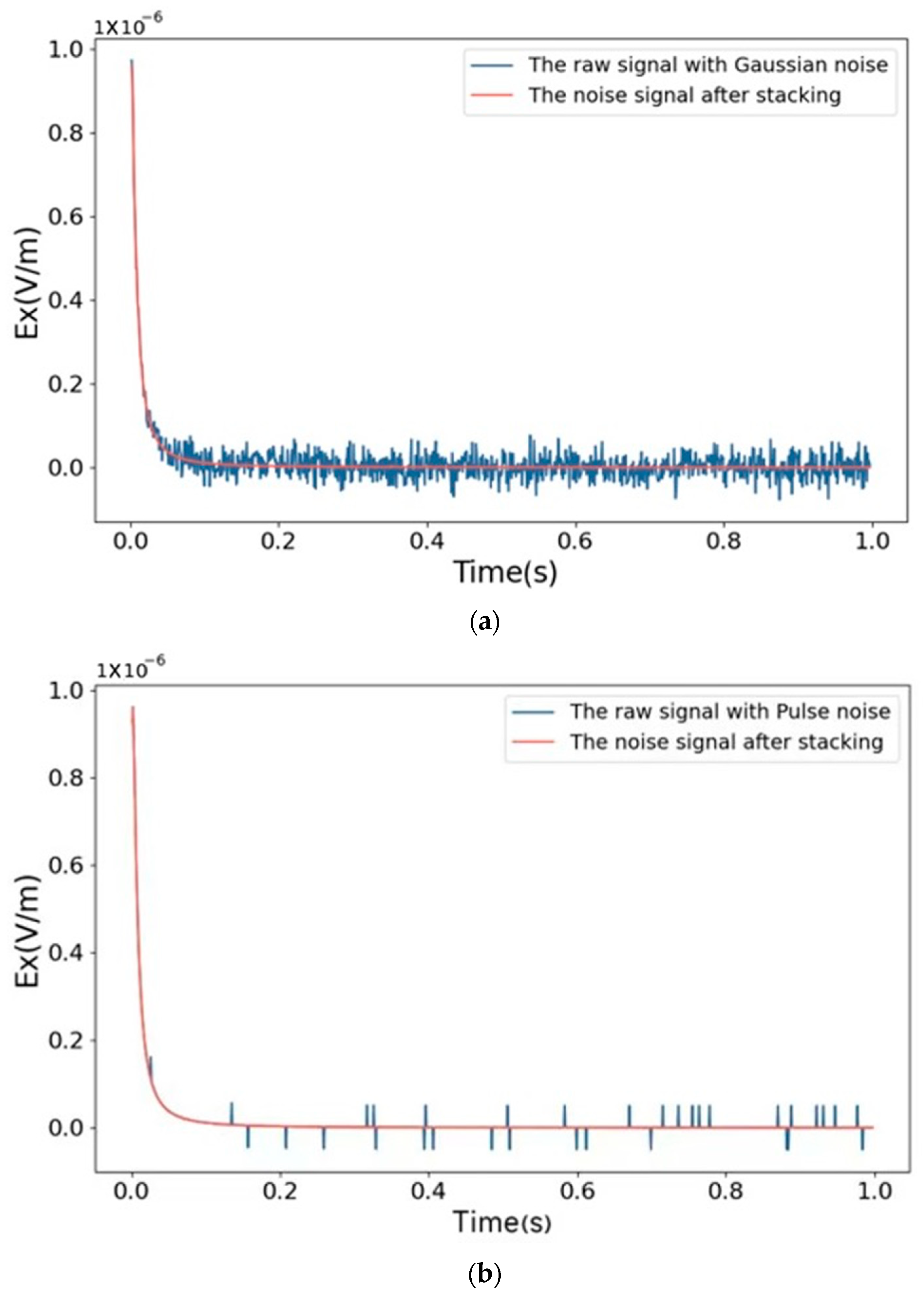
3.1. Effectiveness of Stacking Denoising

To verify the effectiveness of the stacking method, this study employed the 3D forward modeling algorithm of LOTEM [18] to compute theoretical LOTEM response time series comprising 200 time points with a sampling rate of 1000 Hz and a duration of 1 s. Gaussian white noise with a signal-to-noise ratio (SNR) of 10 dB, random impulse noise with an SNR of 20 dB, and frequency noise at 50 Hz were subsequently added to the signals. Figure 3a shows a comparison of the signals before and after stacking with added Gaussian noise, Figure 3b illustrates the signals with added impulse noise before and after stacking, Figure 4a presents the signals with added 50 Hz frequency noise before and after stacking, and Figure 4b shows a comparison of the signals before and after stacking with the three types of noise. As shown in the figure, the stacking method effectively eliminated most Gaussian and impulse noise interference but exhibited limited effectiveness for frequency noise.

The denoising performance of the method was quantitatively assessed using two metrics: root mean square error (RMSE) and signal-to-noise ratio (SNR), defined as follows [19]:

$$RMSE=\sqrt{{\sum }_{i=1}^n{∆d_i}^2/N}$$

(20)

$$SNR=10\times {\log }_{10}\left(sigPower/noisePower\right)$$

(21)

where N is the number of samples, $∆d_i$ represents the difference between the filtered curve and the theoretical forward modeling curve, $sigPower$ denotes the signal power, and $noisePower$ represents the noise power. A smaller RMSE value indicates a higher similarity between the two signals, while a higher SNR reflects better noise reduction performance.

Table 1. Comparison of RMSE and SNR before and after stacking denoising method.

Signal	RMSE	SNR
Simulated noisy signal (Gaussian)	4.39 × 10−8	10
Signal after stacking Denoising	5.65 × 10−9	38.16
Simulated noisy signal (Pulse)	1.81 × 10−8	16.41
Signal after stacking denoising	4.84 × 10−10	44.05
Simulated noisy signal (Frequency)	1.16 × 10−8	14.36
Signal after stacking denoising	1.52 × 10−8	15.05
Simulated noisy signal (three types of noise)	2.98 × 10−08	8.29
Signal after stacking denoising	1.41 × 10−08	14.77

presents the root mean square error and signal-to-noise ratio of the simulated noisy signals before and after denoising. The results demonstrate that for signals with added Gaussian noise and impulse noise, the RMSE significantly decreased, and the SNR substantially increased after signal stacking. However, for signals with added frequency noise, the changes in RMSE and SNR before and after stacking were negligible. This indicates that the stacking method is effective in suppressing Gaussian and impulse noise.

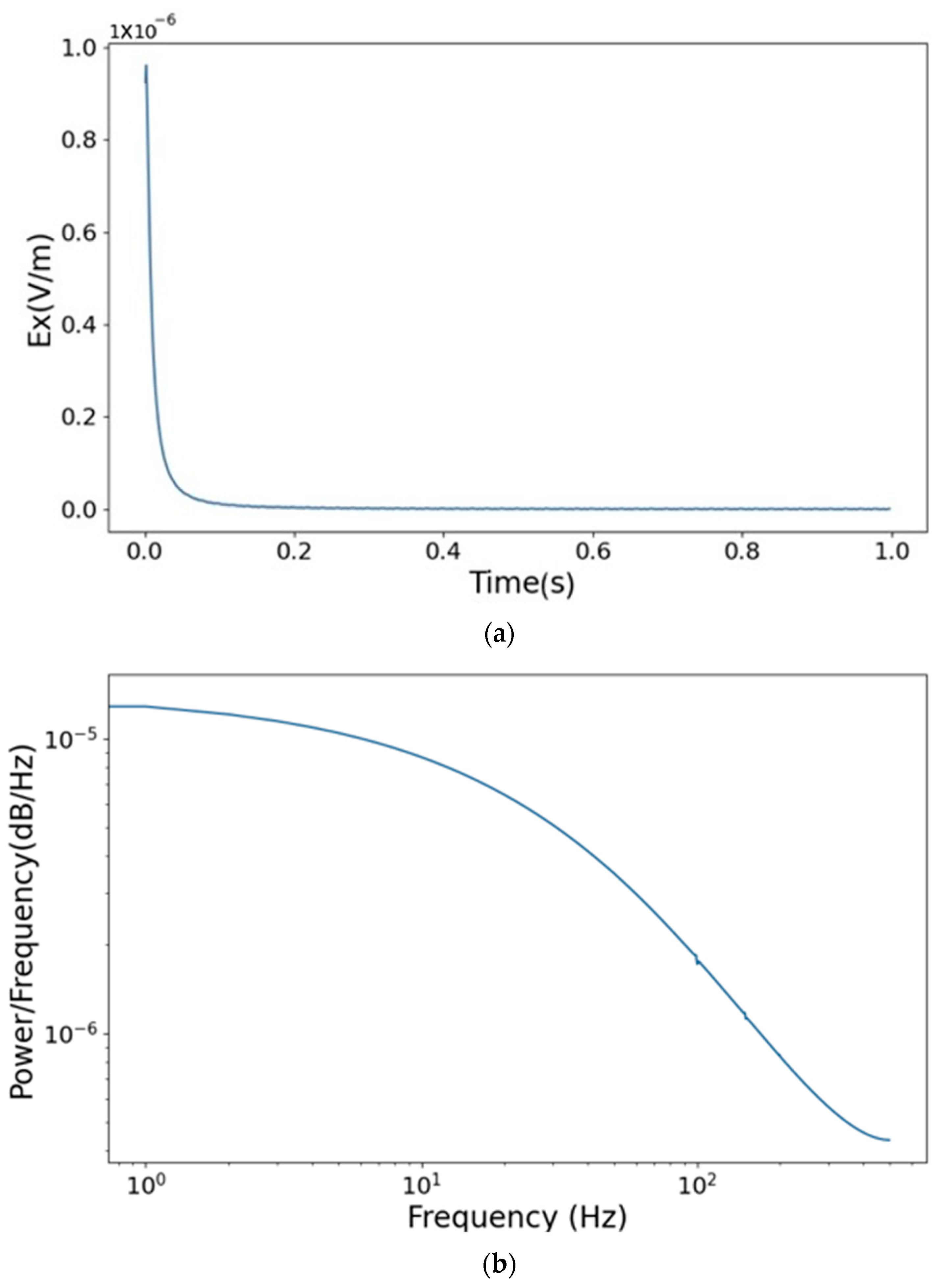
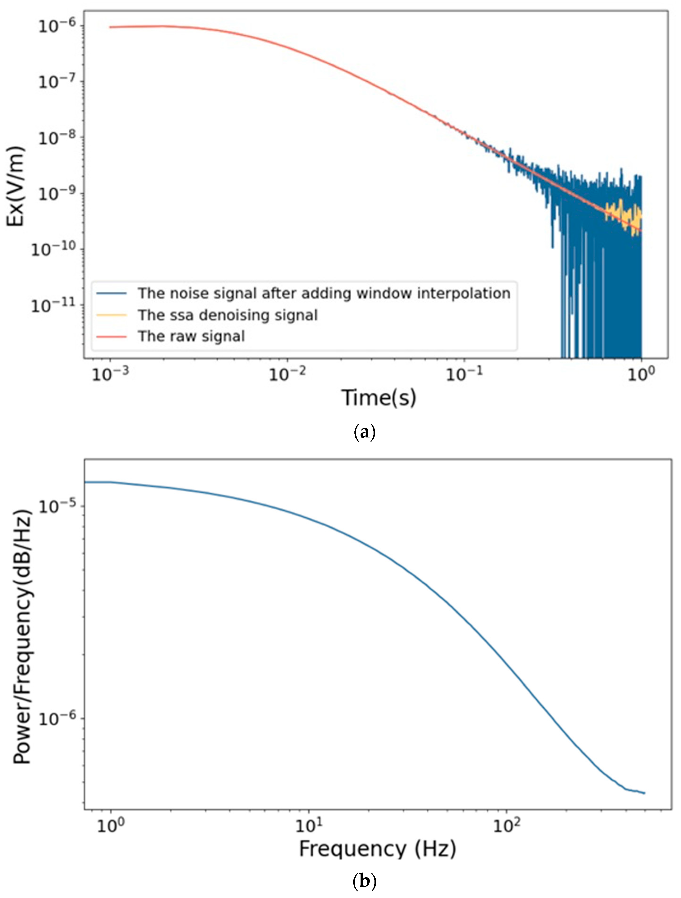
3.2. Effectiveness of Windowed Interpolation

To validate the effectiveness of the windowed interpolation method, 50 Hz frequency noise and its harmonics were added to the theoretical forward response time series (as shown in Figure 5). As illustrated in Figure 6, after windowing, the method successfully identified the 50 Hz frequency noise and its harmonics, marking their main lobes. The algorithm sequentially detected periodic noise at 50 Hz, 100 Hz, 200 Hz, and 150 Hz and effectively eliminated it, achieving a significant noise reduction effect. Furthermore, Figure 7 displays the signal attenuation curve after denoising using the windowed interpolation method, where most of the 50 Hz frequency noise and its harmonics have been effectively removed [11].

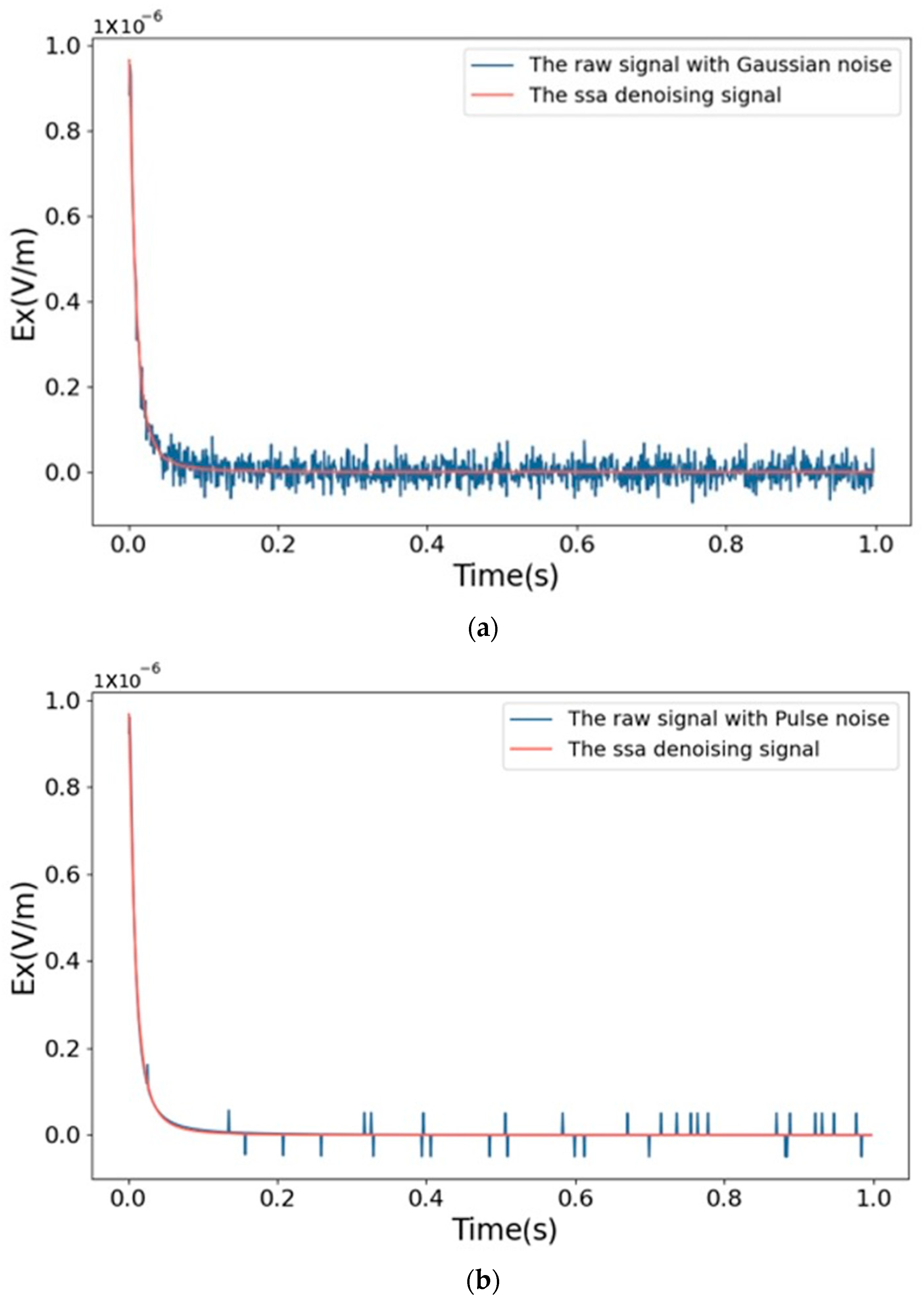
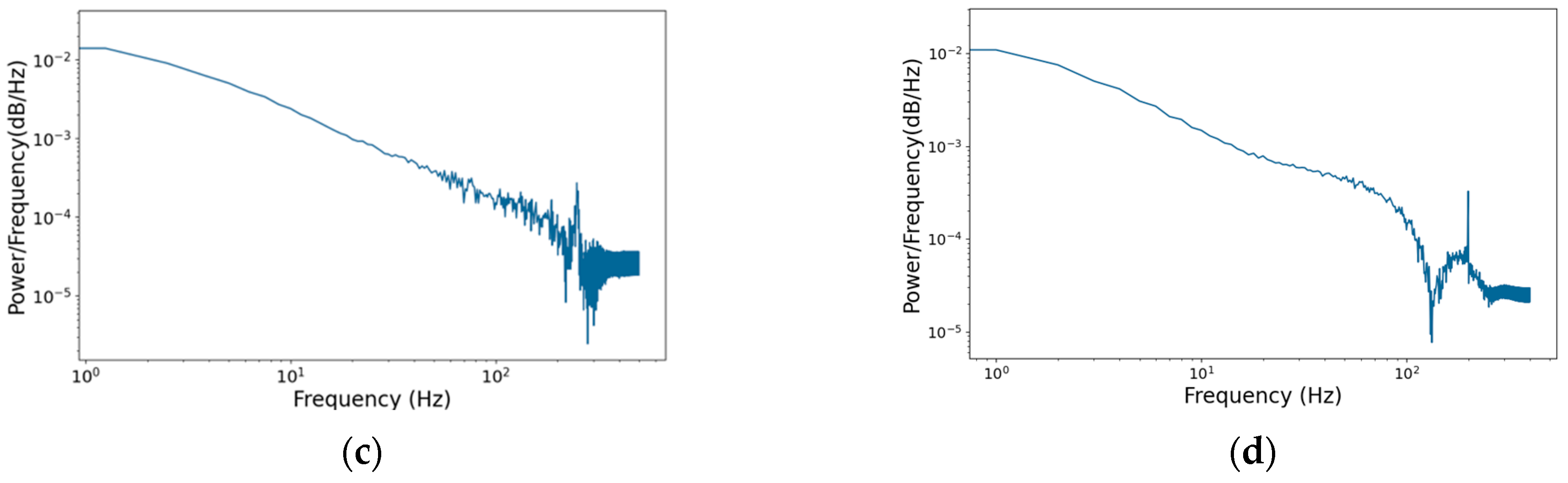
3.3. Effectiveness of SSA

To validate the effectiveness of the singular spectrum analysis (SSA) method, Gaussian white noise with a signal-to-noise ratio (SNR) of 10 dB and random impulse noise with an SNR of 20 dB were respectively added to the theoretical forward response time series (as shown in Figure 7) and then denoised using SSA. The figure demonstrates that most of the Gaussian and impulse noise was effectively removed.

Table 2. Signal-to-noise ratio and RMSE after SSA denoising.

Signal	RMSE	SNR
Simulated noisy signal (Gaussian)	7.46 × 10−9	11.16
SSA denoised signal (Gaussian)	2.76 × 10−9	24.78
Simulated noisy signal (Pulse)	8.37 × 10−9	23.17
SSA denoised signal (Pulse)	1.26 × 10−9	35.64

presents the root mean square error (RMSE) and SNR of the signals after denoising with SSA. The results show significant improvements in both RMSE and SNR, confirming the effectiveness of this method.

As the final step in the signal denoising workflow, the singular spectrum analysis (SSA) method not only removes noise but also enhances the overall smoothing of the signal. To further verify the denoising effectiveness of SSA, the method was applied to a signal after denoising with stacking and windowed interpolation (see Figure 8). From the figure, it can be observed that prior to 0.5 s, the SSA-denoised signal closely aligns with the original signal, while the fitting performance slightly decreases after 0.5 s. After only stacking and windowed interpolation, the signal’s root mean square error (RMSE) was 6.54 × 10⁻¹⁰, and the signal-to-noise ratio (SNR) was 41. After applying SSA, the RMSE was reduced to 3.59 × 10⁻¹⁰, and the SNR significantly increased to 46.66. These results indicate that SSA can further improve signal quality based on the preceding steps [10,20].

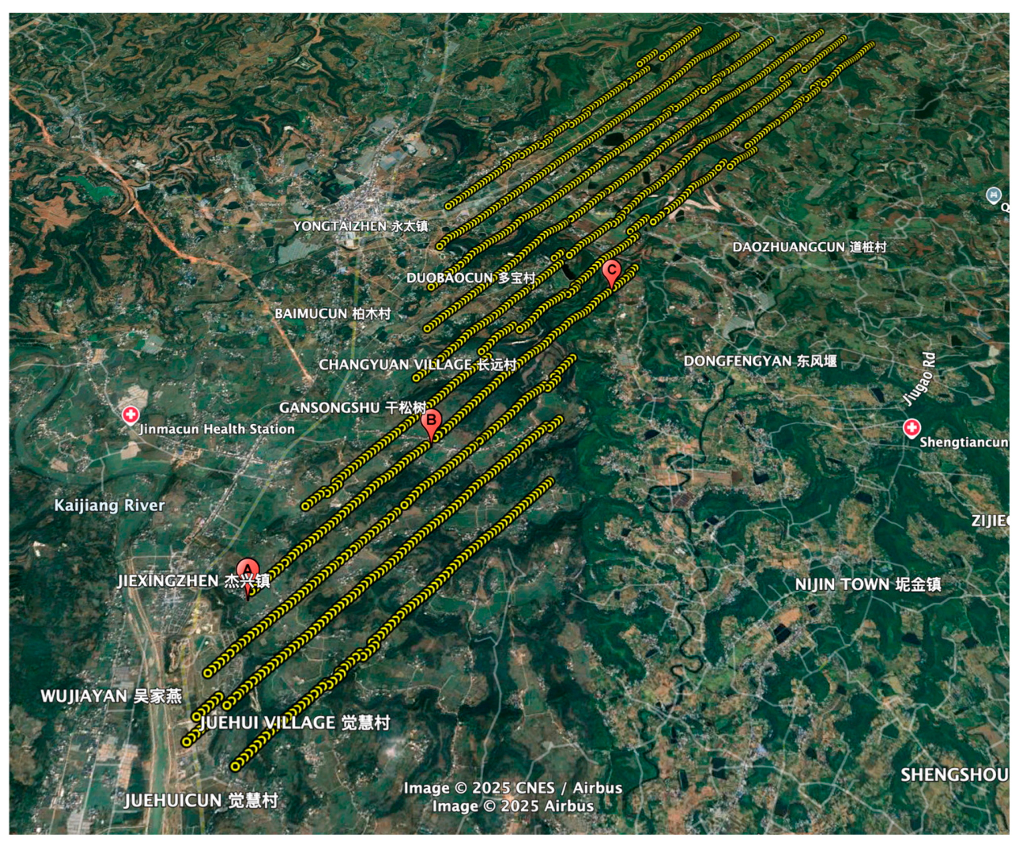
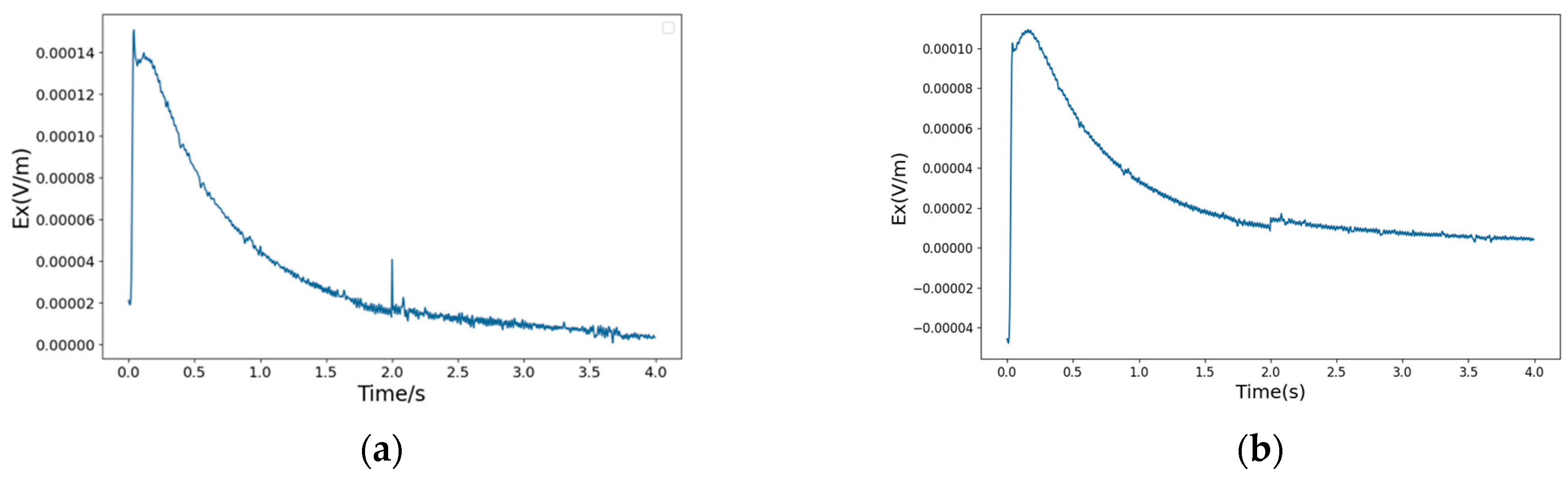
4. Denoising Processing of Field-Measured Data

The measured data used in this study were obtained from Zhongjiang County, Sichuan Province, China. The distribution of the measurement points and lines is shown in Figure 9. The data acquisition instrument used was the V8 system, produced by Phoenix Geophysics in Canada. Noise sources around the entire survey area included human-related noise from villages and towns, noise from substations, and noise from oil wells. Figure 10 presents the data and frequency spectrum for one of the measurement points.

Figure 11a,b show the secondary field decay curves after multi-cycle and polarity-based stacking, while Figure 11c,d display the corresponding spectra. As observed, random pulse interference is suppressed to some extent, and the “spikes” on the curve are significantly reduced. However, the spectra still reveal the presence of prominent power-frequency noise.

Figure 12 shows that after applying the windowed interpolation method for denoising, the decay curve becomes further convergent and smoother, with power-frequency noise significantly suppressed. In Figure 13, the blue curve represents the signal after denoising with the windowed interpolation method, while the red curve shows the signal after additional denoising using singular spectrum analysis (SSA). The results clearly demonstrate the improved denoising effect.

To further validate its accuracy, a comparison of the denoising performance of the proposed algorithm and that of the method presented by Xu Y [10] is shown in Figure 14. The secondary field decay curve obtained after denoising using the proposed algorithm appears more continuous and reasonable, demonstrating superior denoising performance.

To denoise measured signals without a noise-free reference, the residual noise energy can be utilized as an indicator to evaluate the denoising performance [21]. Residual noise energy is an important concept in signal processing, representing the remaining noise energy after the denoising process. As shown in the

Table 3. RNE of two signals.

Signal	RNE
Signal a	0.0283
Signal b	0.2261

, the residual noise energy of both measured signals after denoising was below 0.03, indicating that the denoising algorithm achieved significant noise reduction.

5. Conclusions

This study addressed the issue of low signal-to-noise ratios (SNRs) in long-offset transient electromagnetic (LOTEM) signals under complex electromagnetic environments by proposing a denoising method that combines windowed interpolation and singular spectrum analysis (SSA). The preprocessing step using windowed interpolation effectively suppresses high-frequency noise interference. Subsequently, SSA is employed to decompose and reconstruct the signal, extracting its principal components and removing noise. Theoretical analysis and results from real data processing demonstrate that the proposed method significantly improves the SNR of LOTEM signals while preserving their primary characteristic information, offering high denoising accuracy and robustness.

Compared with traditional filtering methods, the proposed approach not only suppresses noise effectively but also better retains the detailed features of the signal, avoiding excessive loss of valid information. Furthermore, the method demonstrates strong adaptability and stability when dealing with intense noise interference in complex electromagnetic environments, providing an effective technical means for high-precision LOTEM signal processing. Future research could integrate other advanced signal processing techniques, such as deep learning and adaptive decomposition, to further enhance the denoising performance and extend the method’s application to other transient electromagnetic signal processing domains.

References

1. Hördt, A.; Druskin, V.L.; Knizhnerman, L.A.; Strack, K.M. Interpretation of 3-D Effects in Long-Offset Transient Electromagnetic (LOTEM) Soundings in the Muensterland Area/Germany. Geophysics 1992, 57, 1127–1137. [Google Scholar] [CrossRef]
2. Wu, X.; Xue, G.Q.; Xiao, P.; Rao, L.T.; Guo, R.; Fang, G.Y. Noise reduction technology of TEM using optimization of instrument sampling function. Chin. J. Geophys. 2017, 60, 3677–3684. [Google Scholar]
3. Strack, K. Exploration with Deep Transient Electromagnetics; Elsevier Science Publishers B V: Amsterdam, The Netherlands, 1992. [Google Scholar]
4. Macnae, J.C.; Lamontagne, Y.; West, G.F. Noise processing techniques for time-domain EM systems. Geophysics 1984, 49, 934–948. [Google Scholar]
5. Ji, Y.; Wu, Q.; Wang, Y.; Lin, J.; Li, D.; Du, S.; Yu, S.; Guan, S. Noise reduction of grounded electrical source airborne transient electromagnetic data using an exponential fitting-adaptive Kalman filter. Explor. Geophys. 2018, 49, 243–252. [Google Scholar]
6. Chen, K.; Pu, X.; Ren, Y.; Qiu, H.; Lin, F.; Zhang, S. TEMDNet: A novel deep denoising network for transient electromagnetic signal with signal-to-image transformation. IEEE Trans. Geosci. Remote Sens. 2020, 60, 1–18. [Google Scholar]
7. Lin, F.; Chen, K.; Wang, X.; Cao, H.; Chen, D.; Chen, F. Denoising stacked autoencoders for transient electromagnetic signal denoising. Nonlinear Process. Geophys. 2019, 26, 13–23. [Google Scholar]
8. Qi, T.; Wei, X.; Feng, G.; Zhang, F.; Zhao, D.; Guo, J. A method for reducing transient electromagnetic noise: Combination of variational mode decomposition and wavelet denoising algorithm. Measurement 2022, 198, 111420. [Google Scholar] [CrossRef]
9. Zhang, X.; Li, W. Suppression of power frequency noise in vibration signals using windowed interpolation method. Noise Vib. Control 2022, 42, 142–147. [Google Scholar]
10. Xu, Y.; Xie, X.; Zhou, L.; Xi, B.; Yan, L. Noise Characteristics and Denoising Methods of Long-Offset Transient Electromagnetic Method. Minerals 2023, 13, 1084. [Google Scholar] [CrossRef]
11. Lu, C.; Xie, X.; Xu, Y. The research on denoising of long-offset transient electromagnetic stacked signals based on windowed interpolation and singular spectrum analysis integration. In Proceedings of the EMIW-2024, Beppu, Japan, 7–13 September 2024. [Google Scholar]
12. Qi, C.; Wang, X. Harmonic parameter estimation based on interpolated FFT algorithm. J. Electr. Eng. 2003, 18, 92–95. [Google Scholar]
13. Pan, W.; Qian, Y.; Zhou, E. Power harmonic measurement theory based on windowed interpolation FFT—(I) Window function study. J. Electr. Eng. 1994, 50–54. [Google Scholar] [CrossRef]
14. Pan, W.; Qian, Y.; Zhou, E. Power harmonic measurement theory based on windowed interpolation FFT—(II) Double interpolation FFT theory. J. Electr. Eng. 1994, 53–56. [Google Scholar] [CrossRef]
15. Qi, C.; Chen, L.; Wang, X. Accurate estimation of grid harmonic parameters using interpolated FFT algorithm. J. Zhejiang Univ. Eng. Ed. 2003, 37, 112–116. [Google Scholar]
16. Jiang, Z.; Ding, Y. Generality and application characteristics of singular spectrum analysis. Acta Meteorol. Sin. 1998, 56, 736–745. [Google Scholar]
17. Dai, H.; Xu, A.; Sun, W. Signal denoising method based on improved singular spectrum analysis. J. Beijing Inst. Technol. 2016, 36, 727–732. [Google Scholar]
18. Zhigljavsky, A. Singular spectrum analysis for time series: Introduction to this special issue. Stat. Its Interface 2010, 3, 255–258. [Google Scholar] [CrossRef]
19. Wang, X.; Yan, L.; Mao, Y.; Huang, X.; Xie, X.; Zhou, L. 3D forward modeling of long-offset transient electromagnetic under undulating topography. J. Jilin Univ. (Earth Sci. Ed.) 2022, 52, 754–766. [Google Scholar] [CrossRef]
20. Yang, Y.; Li, D.; Tong, T.; Zhang, D.; Zhou, Y.; Chen, Y. Denoising controlled-source electromagnetic data using least-squares inversion. Geophysics 2018, 83, E229–E244. [Google Scholar] [CrossRef]
21. Zhong, J.; Song, J.; You, C. Threshold selection wavelet denoising method based on signal-to-noise ratio evaluation. J. Tsinghua Univ. Nat. Sci. Ed. 2014, 259–263. [Google Scholar] [CrossRef]
Figure 1. Workflow of LOTEM signal denoising [10].
Geosciences 15 00121 g001
Figure 2. Singular spectrum analysis flowchart.
Geosciences 15 00121 g002
Figure 3. (a) Comparison of signals before and after stacking with Gaussian noise; (b) comparison of signals before and after stacking with pulse noise.
Geosciences 15 00121 g003
Figure 4. (a) Comparison of signals before and after stacking with power-frequency noise; (b) comparison of signals before and after stacking with three types of noise.
Geosciences 15 00121 g004
Figure 5. (a) Attenuation curve of the original signal and noisy signal; (b) spectrum of the noisy signal.
Geosciences 15 00121 g005
Figure 6. (a) Attenuation curve of the signal after windowed interpolation denoising; (b) spectrum of the signal after windowed interpolation denoising.
Geosciences 15 00121 g006
Figure 7. (a) Comparison of signals before and after SSA denoising with Gaussian noise; (b) comparison of signals before and after SSA denoising with pulse noise.
Geosciences 15 00121 g007
Figure 8. (a) Comparison of the original signal, windowed interpolation-denoised signal, and SSA-denoised signal; (b) the spectrum after SSA denoising.
Geosciences 15 00121 g008
Figure 9. Measurement points and lines.
Geosciences 15 00121 g009
Figure 10. (a) Field-measured data a; (b) field-measured data b; (c) the spectrum of field-measured data from a; (d) the spectrum of field-measured data from b.
Geosciences 15 00121 g010
Figure 11. (a) Signal a after stacking; (b) signal b after stacking; (c) the spectrum of signal a after stacking; (d) the spectrum of signal b after stacking.
Geosciences 15 00121 g011
Figure 12. (a) Signal a after windowed interpolation denoising; (b) signal b after windowed interpolation denoising; (c) the spectrum of signal a after windowed interpolation denoising; (d) the spectrum of signal b after windowed interpolation denoising.
Geosciences 15 00121 g012aGeosciences 15 00121 g012b
Figure 13. (a) Comparison of SSA-denoised signal a; (b) comparison of SSA-denoised signal b; (c) the spectrum of signal a after SSA denoising; (d) the spectrum of signal b after SSA denoising.
Geosciences 15 00121 g013
Figure 14. (a) Comparison of denoising signal a between Xu Y’s [10] algorithm and the proposed denoising algorithm; (b) comparison of denoising signal b between Xu Y’s [10] algorithm and the proposed denoising algorithm.
Geosciences 15 00121 g014