
Load–Settlement Modeling of Micropiled Rafts in Cohesive Soils Using an Artificial Intelligence Technique


Abstract
1. Introduction
1.1. Background of Micropiles
1.2. Artificial Intelligence (AI) Applications
2. Data Used in the Modeling
2.1. Centrifuge Tests and Numerical Simulations by Alnuaim et al. [13,15]
2.2. Large-Scale Tests by Borthakur and Dey [37]
2.3. Physical Model Tests by El Sawwaf et al. [38]
3. The EPR Predictive Model
3.1. Methodology
3.2. Model Development
4. Model Performance and Sensitivity Analyses
5. Further Validation Using a Case Study
6. Strengths and Limitations
7. Conclusions
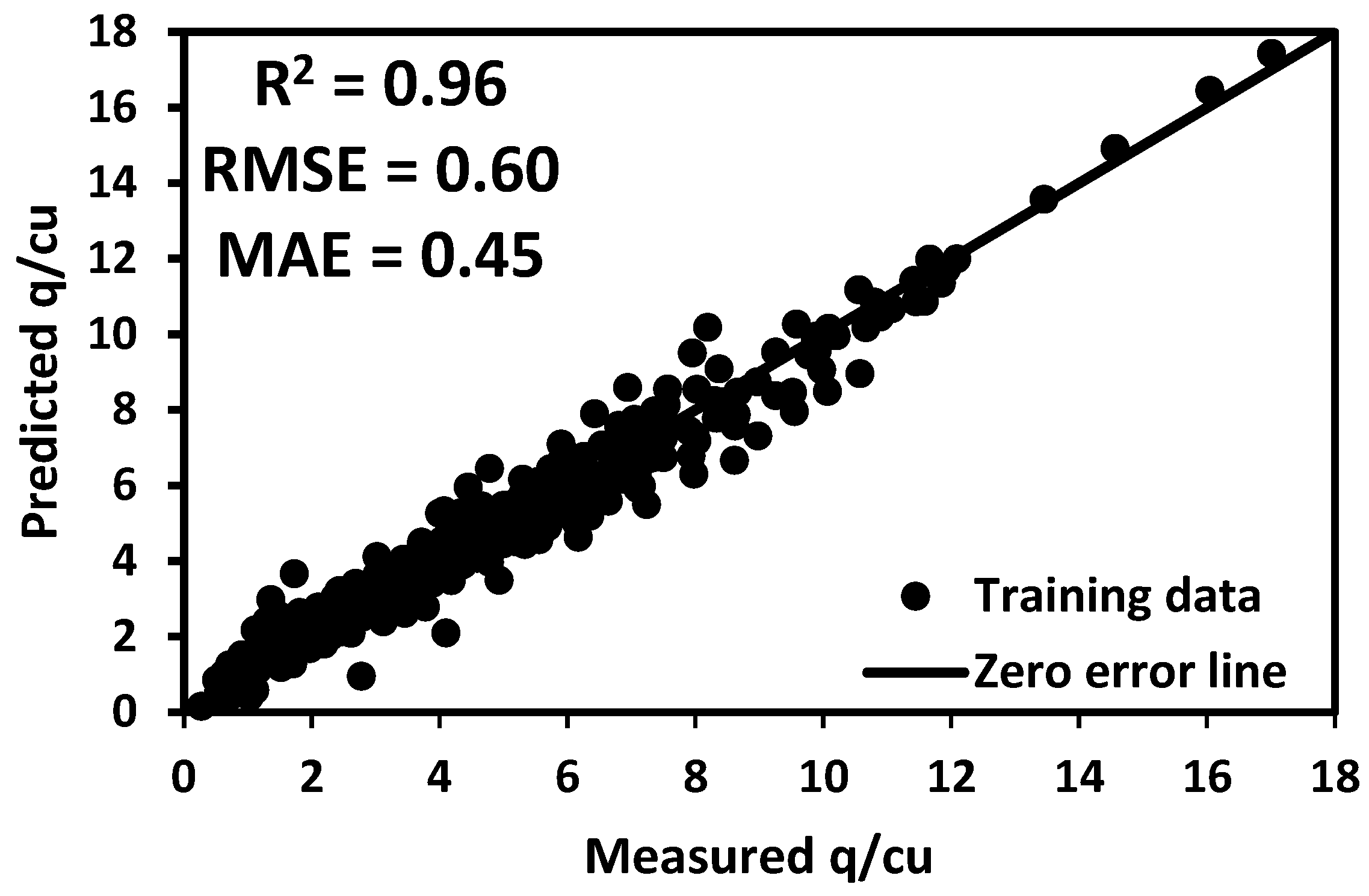
- The model demonstrated excellent performance, with a coefficient of determination (R2) of 0.96 for the training data and 0.93 for the testing data. It effectively captured the nonlinear load–settlement behavior of micropiled rafts.
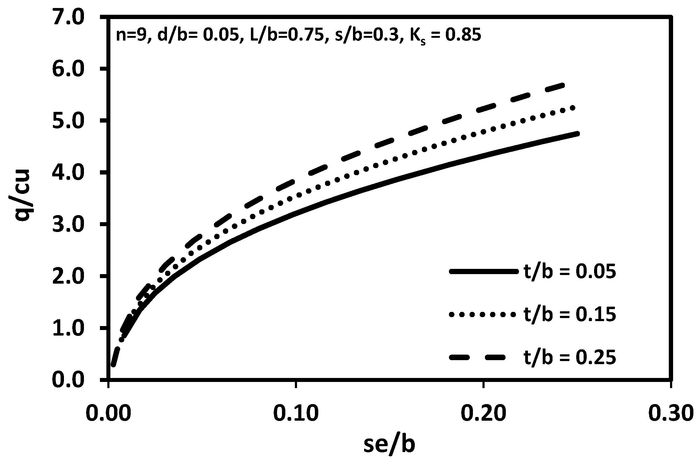
- The sensitivity analyses further validated that the EPR model’s predictions align well with the expected geotechnical behavior. The predicted response of micropiled rafts improves by increasing the micropile length, number, or raft thickness.
- Pressure-grouted micropiles typically exhibit higher values of compared to gravity-grouted ones. This difference reflects the fact that pressure grouting creates greater lateral confinement on the micropile shaft.
- The EPR model was successfully trained to differentiate between the gravity and pressure grouting construction methods, by incorporating the coefficient of lateral earth pressure on the micropile shaft (). A higher bearing capacity could be predicted by using elevated Ks values.
- The model’s sensitivity to was evident in the case study validation, where pressure-grouted micropiles with a higher value (1.5) provided a closer match to field measurements compared to .
Author Contributions
Funding
Data Availability Statement
Conflicts of Interest
Appendix A
Appendix A.1

| d/b | L/b | n | s/b | Ks | t/b | se/b | q/cu |
|---|---|---|---|---|---|---|---|
| 0.0286 | 1.9048 | 4 | 0.2286 | 1.2 | 0.1143 | 0.0003 | 0.2594 |
| 0.0286 | 1.9048 | 4 | 0.2286 | 1.2 | 0.1143 | 0.0006 | 0.5594 |
| 0.0286 | 1.9048 | 4 | 0.2286 | 1.2 | 0.1143 | 0.0009 | 0.8918 |
| 0.0286 | 1.9048 | 4 | 0.2286 | 1.2 | 0.1143 | 0.0014 | 1.3134 |
| 0.0286 | 1.9048 | 4 | 0.2286 | 1.2 | 0.1143 | 0.0018 | 1.6134 |
| 0.0286 | 1.9048 | 4 | 0.2286 | 1.2 | 0.1143 | 0.0023 | 1.9135 |
| 0.0286 | 1.9048 | 4 | 0.2286 | 1.2 | 0.1143 | 0.0028 | 2.2055 |
| 0.0286 | 1.9048 | 4 | 0.2286 | 1.2 | 0.1143 | 0.0035 | 2.4246 |
| 0.0286 | 1.9048 | 4 | 0.2286 | 1.2 | 0.1143 | 0.0042 | 2.6600 |
| 0.0286 | 1.9048 | 4 | 0.2286 | 1.2 | 0.1143 | 0.0051 | 2.8549 |
| 0.0286 | 1.9048 | 4 | 0.2286 | 1.2 | 0.1143 | 0.0059 | 3.0094 |
| 0.0286 | 1.9048 | 4 | 0.2286 | 1.2 | 0.1143 | 0.0070 | 3.1477 |
| 0.0286 | 1.9048 | 4 | 0.2286 | 1.2 | 0.1143 | 0.0079 | 3.2778 |
| 0.0286 | 1.9048 | 4 | 0.2286 | 1.2 | 0.1143 | 0.0090 | 3.4081 |
| 0.0286 | 1.9048 | 4 | 0.2286 | 1.2 | 0.1143 | 0.0102 | 3.5383 |
| 0.0286 | 1.9048 | 4 | 0.2286 | 1.2 | 0.1143 | 0.0115 | 3.7011 |
| 0.0286 | 1.9048 | 4 | 0.2286 | 1.2 | 0.1143 | 0.0124 | 3.7988 |
| 0.0286 | 1.9048 | 4 | 0.2286 | 1.2 | 0.1143 | 0.0133 | 3.8803 |
| 0.0119 | 0.4762 | 289 | 0.0595 | 1.2 | 0.0286 | 0.0036 | 6.0000 |
| 0.0119 | 0.4762 | 121 | 0.0952 | 1.2 | 0.0286 | 0.0036 | 5.0000 |
| 0.0119 | 0.4762 | 81 | 0.119 | 1.2 | 0.0286 | 0.0036 | 4.6667 |
| 0.0119 | 0.4762 | 36 | 0.1905 | 1.2 | 0.0286 | 0.0036 | 4.0000 |
| 0.0119 | 0.4762 | 25 | 0.2381 | 1.2 | 0.0286 | 0.0036 | 3.6667 |
| 0.0119 | 0.4762 | 289 | 0.0595 | 1.2 | 0.0286 | 0.0071 | 8.3330 |
| 0.0119 | 0.4762 | 121 | 0.0952 | 1.2 | 0.0286 | 0.0071 | 6.6667 |
| 0.0119 | 0.4762 | 81 | 0.119 | 1.2 | 0.0286 | 0.0071 | 6.0000 |
| 0.0119 | 0.4762 | 36 | 0.1905 | 1.2 | 0.0286 | 0.0071 | 5.0000 |
| 0.0119 | 0.4762 | 25 | 0.2381 | 1.2 | 0.0286 | 0.0071 | 4.3333 |
| 0.0119 | 0.4762 | 289 | 0.0595 | 1.2 | 0.0143 | 0.0036 | 6.0000 |
| 0.0119 | 0.4762 | 121 | 0.0952 | 1.2 | 0.0143 | 0.0036 | 4.6667 |
| 0.0119 | 0.4762 | 81 | 0.119 | 1.2 | 0.0143 | 0.0036 | 4.3333 |
| 0.0119 | 0.4762 | 36 | 0.1905 | 1.2 | 0.0143 | 0.0036 | 3.6667 |
| 0.0119 | 0.4762 | 25 | 0.2381 | 1.2 | 0.0143 | 0.0036 | 3.3333 |
| 0.0119 | 0.4762 | 289 | 0.0595 | 1.2 | 0.0143 | 0.0071 | 8.0000 |
| 0.0119 | 0.4762 | 121 | 0.0952 | 1.2 | 0.0143 | 0.0071 | 6.3330 |
| 0.0119 | 0.4762 | 81 | 0.119 | 1.2 | 0.0143 | 0.0071 | 5.6667 |
| 0.0119 | 0.4762 | 36 | 0.1905 | 1.2 | 0.0143 | 0.0071 | 4.6667 |
| 0.0119 | 0.4762 | 25 | 0.2381 | 1.2 | 0.0143 | 0.0071 | 4.0000 |
| 0.0119 | 0.4762 | 289 | 0.0595 | 1.2 | 0.0571 | 0.0036 | 6.6667 |
| 0.0119 | 0.4762 | 121 | 0.0952 | 1.2 | 0.0571 | 0.0036 | 5.3333 |
| 0.0119 | 0.4762 | 81 | 0.119 | 1.2 | 0.0571 | 0.0036 | 5.3333 |
| 0.0119 | 0.4762 | 36 | 0.1905 | 1.2 | 0.0571 | 0.0036 | 4.3333 |
| 0.0119 | 0.4762 | 25 | 0.2381 | 1.2 | 0.0571 | 0.0036 | 4.0000 |
| 0.0119 | 0.4762 | 289 | 0.0595 | 1.2 | 0.0571 | 0.0071 | 8.6667 |
| 0.0119 | 0.4762 | 121 | 0.0952 | 1.2 | 0.0571 | 0.0071 | 7.0000 |
| 0.0119 | 0.4762 | 81 | 0.119 | 1.2 | 0.0571 | 0.0071 | 6.0000 |
| 0.0119 | 0.4762 | 36 | 0.1905 | 1.2 | 0.0571 | 0.0071 | 5.0000 |
| 0.0119 | 0.4762 | 25 | 0.2381 | 1.2 | 0.0571 | 0.0071 | 4.6667 |
Appendix A.2
| d/b | L/b | n | s/b | Ks | t/b | se/b | q/cu |
|---|---|---|---|---|---|---|---|
| 0.1695 | 4.0678 | 4 | 0.5085 | 0.5610 | 0.2458 | 0.0003 | 0.6384 |
| 0.1695 | 4.0678 | 4 | 0.5085 | 0.5610 | 0.2458 | 0.0013 | 1.4364 |
| 0.1695 | 4.0678 | 4 | 0.5085 | 0.5610 | 0.2458 | 0.0034 | 2.0428 |
| 0.1695 | 4.0678 | 4 | 0.5085 | 0.5610 | 0.2458 | 0.0067 | 2.5855 |
| 0.1695 | 4.0678 | 4 | 0.5085 | 0.5610 | 0.2458 | 0.0102 | 3.3196 |
| 0.1695 | 4.0678 | 4 | 0.5085 | 0.5610 | 0.2458 | 0.0218 | 3.9516 |
| 0.1695 | 4.0678 | 4 | 0.5085 | 0.5610 | 0.2458 | 0.0407 | 4.4049 |
| 0.1695 | 4.0678 | 4 | 0.5085 | 0.5610 | 0.2458 | 0.0678 | 4.8517 |
| 0.1695 | 4.0678 | 4 | 0.5085 | 0.5610 | 0.2458 | 0.0925 | 5.1901 |
| 0.1695 | 4.0678 | 4 | 0.5085 | 0.5610 | 0.2458 | 0.1153 | 5.4454 |
| 0.1695 | 4.0678 | 4 | 0.5085 | 0.5610 | 0.2458 | 0.1373 | 5.6178 |
| 0.1695 | 4.0678 | 4 | 0.5085 | 0.5610 | 0.2458 | 0.1684 | 5.8476 |
| 0.125 | 3 | 9 | 0.375 | 0.5610 | 0.1813 | 0.001 | 1.0417 |
| 0.125 | 3 | 9 | 0.375 | 0.5610 | 0.1813 | 0.0027 | 2.1938 |
| 0.125 | 3 | 9 | 0.375 | 0.5610 | 0.1813 | 0.0086 | 3.2181 |
| 0.125 | 3 | 9 | 0.375 | 0.5610 | 0.1813 | 0.0275 | 4.5139 |
| 0.125 | 3 | 9 | 0.375 | 0.5610 | 0.1813 | 0.0469 | 5.301 |
| 0.125 | 3 | 9 | 0.375 | 0.5610 | 0.1813 | 0.0763 | 5.9028 |
| 0.125 | 3 | 9 | 0.375 | 0.5610 | 0.1813 | 0.11 | 6.4236 |
| 0.125 | 3 | 9 | 0.375 | 0.5610 | 0.1813 | 0.1456 | 6.9444 |
| 0.0893 | 2.1429 | 16 | 0.2679 | 0.5610 | 0.1295 | 0.0002 | 1.0346 |
| 0.0893 | 2.1429 | 16 | 0.2679 | 0.5610 | 0.1295 | 0.0014 | 2.2003 |
| 0.0893 | 2.1429 | 16 | 0.2679 | 0.5610 | 0.1295 | 0.0063 | 3.2348 |
| 0.0893 | 2.1429 | 16 | 0.2679 | 0.5610 | 0.1295 | 0.0179 | 3.7202 |
| 0.0893 | 2.1429 | 16 | 0.2679 | 0.5610 | 0.1295 | 0.0309 | 4.0745 |
| 0.0893 | 2.1429 | 16 | 0.2679 | 0.5610 | 0.1295 | 0.0443 | 4.4483 |
| 0.0893 | 2.1429 | 16 | 0.2679 | 0.5610 | 0.1295 | 0.0571 | 4.7832 |
| 0.0893 | 2.1429 | 16 | 0.2679 | 0.5610 | 0.1295 | 0.0732 | 5.1375 |
| 0.0893 | 2.1429 | 16 | 0.2679 | 0.5610 | 0.1295 | 0.0864 | 5.4439 |
| 0.1667 | 4 | 4 | 0.75 | 0.5610 | 0.2417 | 0.0003 | 0.7407 |
| 0.1667 | 4 | 4 | 0.75 | 0.5610 | 0.2417 | 0.0008 | 1.7037 |
| 0.1667 | 4 | 4 | 0.75 | 0.5610 | 0.2417 | 0.0038 | 2.7845 |
| 0.1667 | 4 | 4 | 0.75 | 0.5610 | 0.2417 | 0.0159 | 3.9898 |
| 0.1667 | 4 | 4 | 0.75 | 0.5610 | 0.2417 | 0.037 | 4.7115 |
| 0.1667 | 4 | 4 | 0.75 | 0.5610 | 0.2417 | 0.0667 | 5.3086 |
| 0.1667 | 4 | 4 | 0.75 | 0.5610 | 0.2417 | 0.094 | 5.7428 |
| 0.1667 | 4 | 4 | 0.75 | 0.5610 | 0.2417 | 0.128 | 6.1728 |
| 0.1667 | 4 | 4 | 0.75 | 0.5610 | 0.2417 | 0.16 | 6.5432 |
| 0.1667 | 4 | 4 | 0.75 | 0.5610 | 0.2417 | 0.2049 | 7.047 |
| 0.0893 | 2.1429 | 9 | 0.4018 | 0.5610 | 0.1295 | 0.0009 | 0.713 |
| 0.0893 | 2.1429 | 9 | 0.4018 | 0.5610 | 0.1295 | 0.0036 | 1.3287 |
| 0.0893 | 2.1429 | 9 | 0.4018 | 0.5610 | 0.1295 | 0.0068 | 1.729 |
| 0.0893 | 2.1429 | 9 | 0.4018 | 0.5610 | 0.1295 | 0.0107 | 2.2144 |
| 0.0893 | 2.1429 | 9 | 0.4018 | 0.5610 | 0.1295 | 0.0197 | 2.6272 |
| 0.0893 | 2.1429 | 9 | 0.4018 | 0.5610 | 0.1295 | 0.0357 | 3.0116 |
| 0.0893 | 2.1429 | 9 | 0.4018 | 0.5610 | 0.1295 | 0.0623 | 3.4315 |
| 0.0893 | 2.1429 | 9 | 0.4018 | 0.5610 | 0.1295 | 0.0911 | 3.7202 |
| 0.0893 | 2.1429 | 9 | 0.4018 | 0.5610 | 0.1295 | 0.1235 | 3.9718 |
| 0.0658 | 1.5789 | 16 | 0.2961 | 0.5610 | 0.0954 | 0.0006 | 0.6189 |
| 0.0658 | 1.5789 | 16 | 0.2961 | 0.5610 | 0.0954 | 0.0016 | 1.2037 |
| 0.0658 | 1.5789 | 16 | 0.2961 | 0.5610 | 0.0954 | 0.0042 | 1.826 |
| 0.0658 | 1.5789 | 16 | 0.2961 | 0.5610 | 0.0954 | 0.0114 | 2.3615 |
| 0.0658 | 1.5789 | 16 | 0.2961 | 0.5610 | 0.0954 | 0.0201 | 2.8597 |
| 0.0658 | 1.5789 | 16 | 0.2961 | 0.5610 | 0.0954 | 0.0283 | 3.1741 |
| 0.0658 | 1.5789 | 16 | 0.2961 | 0.5610 | 0.0954 | 0.0397 | 3.5595 |
| 0.0658 | 1.5789 | 16 | 0.2961 | 0.5610 | 0.0954 | 0.05 | 3.8582 |
| 0.1429 | 3.4286 | 4 | 0.8571 | 0.5610 | 0.2071 | 0.0004 | 0.5442 |
| 0.1429 | 3.4286 | 4 | 0.8571 | 0.5610 | 0.2071 | 0.0012 | 1.3902 |
| 0.1429 | 3.4286 | 4 | 0.8571 | 0.5610 | 0.2071 | 0.0029 | 2.309 |
| 0.1429 | 3.4286 | 4 | 0.8571 | 0.5610 | 0.2071 | 0.0075 | 3.3596 |
| 0.1429 | 3.4286 | 4 | 0.8571 | 0.5610 | 0.2071 | 0.0262 | 4.3681 |
| 0.1429 | 3.4286 | 4 | 0.8571 | 0.5610 | 0.2071 | 0.0571 | 4.9887 |
| 0.1429 | 3.4286 | 4 | 0.8571 | 0.5610 | 0.2071 | 0.0815 | 5.3446 |
| 0.1429 | 3.4286 | 4 | 0.8571 | 0.5610 | 0.2071 | 0.1011 | 5.6236 |
| 0.1429 | 3.4286 | 4 | 0.8571 | 0.5610 | 0.2071 | 0.1371 | 6.0771 |
| 0.1429 | 3.4286 | 4 | 0.8571 | 0.5610 | 0.2071 | 0.1602 | 6.3581 |
| 0.0667 | 1.6 | 9 | 0.4 | 0.5610 | 0.0967 | 0.0004 | 0.5378 |
| 0.0667 | 1.6 | 9 | 0.4 | 0.5610 | 0.0967 | 0.0014 | 1.044 |
| 0.0667 | 1.6 | 9 | 0.4 | 0.5610 | 0.0967 | 0.0056 | 1.6258 |
| 0.0667 | 1.6 | 9 | 0.4 | 0.5610 | 0.0967 | 0.0114 | 2.1944 |
| 0.0667 | 1.6 | 9 | 0.4 | 0.5610 | 0.0967 | 0.0177 | 2.6168 |
| 0.0667 | 1.6 | 9 | 0.4 | 0.5610 | 0.0967 | 0.0278 | 3.12 |
| 0.0667 | 1.6 | 9 | 0.4 | 0.5610 | 0.0967 | 0.0377 | 3.4568 |
| 0.0667 | 1.6 | 9 | 0.4 | 0.5610 | 0.0967 | 0.0473 | 3.7824 |
| 0.0495 | 1.1881 | 16 | 0.297 | 0.5610 | 0.0718 | 0.0004 | 0.2723 |
| 0.0495 | 1.1881 | 16 | 0.297 | 0.5610 | 0.0718 | 0.0009 | 0.5462 |
| 0.0495 | 1.1881 | 16 | 0.297 | 0.5610 | 0.0718 | 0.0013 | 0.6808 |
| 0.0495 | 1.1881 | 16 | 0.297 | 0.5610 | 0.0718 | 0.002 | 1.0072 |
| 0.0495 | 1.1881 | 16 | 0.297 | 0.5610 | 0.0718 | 0.0026 | 1.15 |
| 0.0495 | 1.1881 | 16 | 0.297 | 0.5610 | 0.0718 | 0.0041 | 1.4944 |
| 0.0495 | 1.1881 | 16 | 0.297 | 0.5610 | 0.0718 | 0.0061 | 1.7486 |
| 0.0495 | 1.1881 | 16 | 0.297 | 0.5610 | 0.0718 | 0.0098 | 2.0751 |
| 0.0495 | 1.1881 | 16 | 0.297 | 0.5610 | 0.0718 | 0.0131 | 2.2874 |
| 0.0495 | 1.1881 | 16 | 0.297 | 0.5610 | 0.0718 | 0.0166 | 2.4914 |
| 0.0495 | 1.1881 | 16 | 0.297 | 0.5610 | 0.0718 | 0.0198 | 2.6141 |
| 0.0495 | 1.1881 | 16 | 0.297 | 0.5610 | 0.0718 | 0.0234 | 2.7128 |
| 0.1667 | 5.3333 | 4 | 0.5 | 0.5610 | 0.2417 | 0.0008 | 1.2346 |
| 0.1667 | 5.3333 | 4 | 0.5 | 0.5610 | 0.2417 | 0.0021 | 2.6694 |
| 0.1667 | 5.3333 | 4 | 0.5 | 0.5610 | 0.2417 | 0.0027 | 3.7037 |
| 0.1667 | 5.3333 | 4 | 0.5 | 0.5610 | 0.2417 | 0.0046 | 4.9333 |
| 0.1667 | 5.3333 | 4 | 0.5 | 0.5610 | 0.2417 | 0.0123 | 6.1728 |
| 0.1667 | 5.3333 | 4 | 0.5 | 0.5610 | 0.2417 | 0.0332 | 7.1014 |
| 0.1667 | 5.3333 | 4 | 0.5 | 0.5610 | 0.2417 | 0.0767 | 8.0247 |
| 0.1667 | 5.3333 | 4 | 0.5 | 0.5610 | 0.2417 | 0.1143 | 8.642 |
| 0.1667 | 5.3333 | 4 | 0.5 | 0.5610 | 0.2417 | 0.15 | 9.2593 |
| 0.1667 | 5.3333 | 4 | 0.5 | 0.5610 | 0.2417 | 0.1891 | 9.8778 |
| 0.125 | 4 | 9 | 0.375 | 0.5610 | 0.1813 | 0.0002 | 2.7778 |
| 0.125 | 4 | 9 | 0.375 | 0.5610 | 0.1813 | 0.0007 | 4.1014 |
| 0.125 | 4 | 9 | 0.375 | 0.5610 | 0.1813 | 0.0027 | 5.454 |
| 0.125 | 4 | 9 | 0.375 | 0.5610 | 0.1813 | 0.0139 | 7.2396 |
| 0.125 | 4 | 9 | 0.375 | 0.5610 | 0.1813 | 0.0263 | 8.1597 |
| 0.125 | 4 | 9 | 0.375 | 0.5610 | 0.1813 | 0.0417 | 8.9788 |
| 0.125 | 4 | 9 | 0.375 | 0.5610 | 0.1813 | 0.0575 | 9.5486 |
| 0.125 | 4 | 9 | 0.375 | 0.5610 | 0.1813 | 0.0733 | 10.069 |
| 0.125 | 4 | 9 | 0.375 | 0.5610 | 0.1813 | 0.0896 | 10.576 |
| 0.1563 | 5 | 4 | 0.7031 | 0.5610 | 0.2266 | 0.0003 | 0.651 |
| 0.1563 | 5 | 4 | 0.7031 | 0.5610 | 0.2266 | 0.0007 | 1.5516 |
| 0.1563 | 5 | 4 | 0.7031 | 0.5610 | 0.2266 | 0.0019 | 2.7669 |
| 0.1563 | 5 | 4 | 0.7031 | 0.5610 | 0.2266 | 0.0025 | 3.3637 |
| 0.1563 | 5 | 4 | 0.7031 | 0.5610 | 0.2266 | 0.0041 | 4.1829 |
| 0.1563 | 5 | 4 | 0.7031 | 0.5610 | 0.2266 | 0.0141 | 4.8828 |
| 0.1563 | 5 | 4 | 0.7031 | 0.5610 | 0.2266 | 0.0236 | 5.3993 |
| 0.1563 | 5 | 4 | 0.7031 | 0.5610 | 0.2266 | 0.0431 | 6.1051 |
| 0.1563 | 5 | 4 | 0.7031 | 0.5610 | 0.2266 | 0.0765 | 6.8229 |
| 0.1563 | 5 | 4 | 0.7031 | 0.5610 | 0.2266 | 0.0938 | 7.053 |
| 0.1563 | 5 | 4 | 0.7031 | 0.5610 | 0.2266 | 0.1141 | 7.27 |
| 0.1563 | 5 | 4 | 0.7031 | 0.5610 | 0.2266 | 0.1425 | 7.5684 |
| 0.0909 | 2.9091 | 9 | 0.4091 | 0.5610 | 0.1318 | 0.0009 | 0.9183 |
| 0.0909 | 2.9091 | 9 | 0.4091 | 0.5610 | 0.1318 | 0.0025 | 1.844 |
| 0.0909 | 2.9091 | 9 | 0.4091 | 0.5610 | 0.1318 | 0.0058 | 2.7548 |
| 0.0909 | 2.9091 | 9 | 0.4091 | 0.5610 | 0.1318 | 0.011 | 3.5152 |
| 0.0909 | 2.9091 | 9 | 0.4091 | 0.5610 | 0.1318 | 0.0182 | 4.1322 |
| 0.0909 | 2.9091 | 9 | 0.4091 | 0.5610 | 0.1318 | 0.0255 | 4.5914 |
| 0.0909 | 2.9091 | 9 | 0.4091 | 0.5610 | 0.1318 | 0.0387 | 5.1978 |
| 0.0909 | 2.9091 | 9 | 0.4091 | 0.5610 | 0.1318 | 0.0551 | 5.6933 |
| 0.0909 | 2.9091 | 9 | 0.4091 | 0.5610 | 0.1318 | 0.0727 | 6.1524 |
| 0.0909 | 2.9091 | 9 | 0.4091 | 0.5610 | 0.1318 | 0.0949 | 6.6412 |
| 0.125 | 4 | 4 | 0.75 | 0.5610 | 0.1813 | 0.0004 | 1.0417 |
| 0.125 | 4 | 4 | 0.75 | 0.5610 | 0.1813 | 0.0009 | 1.8392 |
| 0.125 | 4 | 4 | 0.75 | 0.5610 | 0.1813 | 0.0045 | 2.7778 |
| 0.125 | 4 | 4 | 0.75 | 0.5610 | 0.1813 | 0.013 | 3.5888 |
| 0.125 | 4 | 4 | 0.75 | 0.5610 | 0.1813 | 0.0345 | 4.5139 |
| 0.125 | 4 | 4 | 0.75 | 0.5610 | 0.1813 | 0.0611 | 5.2365 |
| 0.125 | 4 | 4 | 0.75 | 0.5610 | 0.1813 | 0.09 | 5.7292 |
| 0.125 | 4 | 4 | 0.75 | 0.5610 | 0.1813 | 0.125 | 6.25 |
| 0.125 | 4 | 4 | 0.75 | 0.5610 | 0.1813 | 0.1591 | 6.7275 |
| 0.0714 | 2.2857 | 9 | 0.4286 | 0.5610 | 0.1036 | 0.0009 | 0.5669 |
| 0.0714 | 2.2857 | 9 | 0.4286 | 0.5610 | 0.1036 | 0.0019 | 1.01633 |
| 0.0714 | 2.2857 | 9 | 0.4286 | 0.5610 | 0.1036 | 0.0029 | 1.5873 |
| 0.0714 | 2.2857 | 9 | 0.4286 | 0.5610 | 0.1036 | 0.0063 | 2.20321 |
| 0.0714 | 2.2857 | 9 | 0.4286 | 0.5610 | 0.1036 | 0.0157 | 2.83447 |
| 0.0714 | 2.2857 | 9 | 0.4286 | 0.5610 | 0.1036 | 0.0304 | 3.40332 |
| 0.0714 | 2.2857 | 9 | 0.4286 | 0.5610 | 0.1036 | 0.0429 | 3.68481 |
| 0.0714 | 2.2857 | 9 | 0.4286 | 0.5610 | 0.1036 | 0.06 | 3.96825 |
| 0.0714 | 2.2857 | 9 | 0.4286 | 0.5610 | 0.1036 | 0.0855 | 4.37501 |
| 0.1667 | 6.6667 | 4 | 0.5 | 0.5610 | 0.2417 | 0.0003 | 1.8179 |
| 0.1667 | 6.6667 | 4 | 0.5 | 0.5610 | 0.2417 | 0.0021 | 3.95679 |
| 0.1667 | 6.6667 | 4 | 0.5 | 0.5610 | 0.2417 | 0.0083 | 5.55556 |
| 0.1667 | 6.6667 | 4 | 0.5 | 0.5610 | 0.2417 | 0.0192 | 6.83642 |
| 0.1667 | 6.6667 | 4 | 0.5 | 0.5610 | 0.2417 | 0.0367 | 8.02469 |
| 0.1667 | 6.6667 | 4 | 0.5 | 0.5610 | 0.2417 | 0.06 | 9.25926 |
| 0.1667 | 6.6667 | 4 | 0.5 | 0.5610 | 0.2417 | 0.0799 | 10.0877 |
| 0.1667 | 6.6667 | 4 | 0.5 | 0.5610 | 0.2417 | 0.1067 | 10.8025 |
| 0.1667 | 6.6667 | 4 | 0.5 | 0.5610 | 0.2417 | 0.1333 | 11.4198 |
| 0.1667 | 6.6667 | 4 | 0.5 | 0.5610 | 0.2417 | 0.164 | 12.0889 |
| 0.1111 | 4.4444 | 9 | 0.3333 | 0.5610 | 0.1611 | 0.0004 | 1.48486 |
| 0.1111 | 4.4444 | 9 | 0.3333 | 0.5610 | 0.1611 | 0.0019 | 2.63336 |
| 0.1111 | 4.4444 | 9 | 0.3333 | 0.5610 | 0.1611 | 0.0067 | 4.049 |
| 0.1111 | 4.4444 | 9 | 0.3333 | 0.5610 | 0.1611 | 0.0117 | 5.2594 |
| 0.1111 | 4.4444 | 9 | 0.3333 | 0.5610 | 0.1611 | 0.0222 | 6.39232 |
| 0.1111 | 4.4444 | 9 | 0.3333 | 0.5610 | 0.1611 | 0.0462 | 7.22908 |
| 0.1111 | 4.4444 | 9 | 0.3333 | 0.5610 | 0.1611 | 0.0756 | 7.54458 |
| 0.1111 | 4.4444 | 9 | 0.3333 | 0.5610 | 0.1611 | 0.1156 | 7.81893 |
| 0.1111 | 4.4444 | 9 | 0.3333 | 0.5610 | 0.1611 | 0.1444 | 7.9561 |
| 0.1111 | 4.4444 | 9 | 0.3333 | 0.5610 | 0.1611 | 0.1903 | 8.19479 |
| 0.1429 | 5.7143 | 4 | 0.6429 | 0.5610 | 0.2071 | 0.0017 | 1.36054 |
| 0.1429 | 5.7143 | 4 | 0.6429 | 0.5610 | 0.2071 | 0.0046 | 3.02222 |
| 0.1429 | 5.7143 | 4 | 0.6429 | 0.5610 | 0.2071 | 0.0086 | 4.30839 |
| 0.1429 | 5.7143 | 4 | 0.6429 | 0.5610 | 0.2071 | 0.0267 | 5.73787 |
| 0.1429 | 5.7143 | 4 | 0.6429 | 0.5610 | 0.2071 | 0.0543 | 6.80272 |
| 0.1429 | 5.7143 | 4 | 0.6429 | 0.5610 | 0.2071 | 0.0886 | 7.93651 |
| 0.1429 | 5.7143 | 4 | 0.6429 | 0.5610 | 0.2071 | 0.1419 | 9.4381 |
| 0.1429 | 5.7143 | 4 | 0.6429 | 0.5610 | 0.2071 | 0.1771 | 10.2041 |
| 0.1429 | 5.7143 | 4 | 0.6429 | 0.5610 | 0.2071 | 0.2171 | 10.8844 |
| 0.1429 | 5.7143 | 4 | 0.6429 | 0.5610 | 0.2071 | 0.2543 | 11.4522 |
| 0.0926 | 3.7037 | 9 | 0.4167 | 0.5610 | 0.1343 | 0.0013 | 1.11797 |
| 0.0926 | 3.7037 | 9 | 0.4167 | 0.5610 | 0.1343 | 0.0041 | 2.4257 |
| 0.0926 | 3.7037 | 9 | 0.4167 | 0.5610 | 0.1343 | 0.0081 | 3.46174 |
| 0.0926 | 3.7037 | 9 | 0.4167 | 0.5610 | 0.1343 | 0.013 | 4.28669 |
| 0.0926 | 3.7037 | 9 | 0.4167 | 0.5610 | 0.1343 | 0.0179 | 4.83482 |
| 0.0926 | 3.7037 | 9 | 0.4167 | 0.5610 | 0.1343 | 0.0265 | 5.52507 |
| 0.0926 | 3.7037 | 9 | 0.4167 | 0.5610 | 0.1343 | 0.0396 | 6.14426 |
| 0.0926 | 3.7037 | 9 | 0.4167 | 0.5610 | 0.1343 | 0.0556 | 6.57293 |
| 0.0926 | 3.7037 | 9 | 0.4167 | 0.5610 | 0.1343 | 0.0722 | 6.95397 |
| 0.0926 | 3.7037 | 9 | 0.4167 | 0.5610 | 0.1343 | 0.0881 | 7.27176 |
| 0.2 | 5 | 4 | 0.6 | 0.5610 | 0.4833 | 0.0027 | 1.7284 |
| 0.2 | 5 | 4 | 0.6 | 0.5610 | 0.4833 | 0.008 | 3.7284 |
| 0.2 | 5 | 4 | 0.6 | 0.5610 | 0.4833 | 0.0167 | 5.92593 |
| 0.2 | 5 | 4 | 0.6 | 0.5610 | 0.4833 | 0.0233 | 7.90124 |
| 0.2 | 5 | 4 | 0.6 | 0.5610 | 0.4833 | 0.044 | 9.98025 |
| 0.2 | 5 | 4 | 0.6 | 0.5610 | 0.4833 | 0.09 | 11.8519 |
| 0.2 | 5 | 4 | 0.6 | 0.5610 | 0.4833 | 0.156 | 13.4568 |
| 0.2 | 5 | 4 | 0.6 | 0.5610 | 0.4833 | 0.2067 | 14.5679 |
| 0.2 | 5 | 4 | 0.6 | 0.5610 | 0.4833 | 0.2753 | 16.0494 |
| 0.2 | 5 | 4 | 0.6 | 0.5610 | 0.4833 | 0.3249 | 17.0124 |
| 0.12 | 3 | 9 | 0.36 | 0.5610 | 0.2900 | 0.0024 | 1.51111 |
| 0.12 | 3 | 9 | 0.36 | 0.5610 | 0.2900 | 0.004 | 2.84444 |
| 0.12 | 3 | 9 | 0.36 | 0.5610 | 0.2900 | 0.0102 | 4.26133 |
| 0.12 | 3 | 9 | 0.36 | 0.5610 | 0.2900 | 0.02 | 6.04444 |
| 0.12 | 3 | 9 | 0.36 | 0.5610 | 0.2900 | 0.0432 | 7.50133 |
| 0.12 | 3 | 9 | 0.36 | 0.5610 | 0.2900 | 0.088 | 8.88889 |
| 0.12 | 3 | 9 | 0.36 | 0.5610 | 0.2900 | 0.124 | 9.77778 |
| 0.12 | 3 | 9 | 0.36 | 0.5610 | 0.2900 | 0.1787 | 11.0711 |
| 0.0857 | 2.1429 | 16 | 0.2571 | 0.5610 | 0.2071 | 0.0009 | 0.90703 |
| 0.0857 | 2.1429 | 16 | 0.2571 | 0.5610 | 0.2071 | 0.0024 | 2.04082 |
| 0.0857 | 2.1429 | 16 | 0.2571 | 0.5610 | 0.2071 | 0.0054 | 3.1746 |
| 0.0857 | 2.1429 | 16 | 0.2571 | 0.5610 | 0.2071 | 0.0092 | 3.99683 |
| 0.0857 | 2.1429 | 16 | 0.2571 | 0.5610 | 0.2071 | 0.0137 | 4.98866 |
| 0.0857 | 2.1429 | 16 | 0.2571 | 0.5610 | 0.2071 | 0.02 | 6.12245 |
| 0.0857 | 2.1429 | 16 | 0.2571 | 0.5610 | 0.2071 | 0.0333 | 7.161 |
| 0.0857 | 2.1429 | 16 | 0.2571 | 0.5610 | 0.2071 | 0.0486 | 7.93651 |
| 0.0857 | 2.1429 | 16 | 0.2571 | 0.5610 | 0.2071 | 0.0671 | 8.61678 |
| 0.0857 | 2.1429 | 16 | 0.2571 | 0.5610 | 0.2071 | 0.0929 | 9.52381 |
| 0.0857 | 2.1429 | 16 | 0.2571 | 0.5610 | 0.2071 | 0.1172 | 10.3444 |
| 0.13 | 3.75 | 4 | 0.6 | 0.5610 | 0.3625 | 0.0003 | 0.83333 |
| 0.13 | 3.75 | 4 | 0.6 | 0.5610 | 0.3625 | 0.0006 | 1.70556 |
| 0.13 | 3.75 | 4 | 0.6 | 0.5610 | 0.3625 | 0.0078 | 2.89139 |
| 0.13 | 3.75 | 4 | 0.6 | 0.5610 | 0.3625 | 0.015 | 3.88889 |
| 0.13 | 3.75 | 4 | 0.6 | 0.5610 | 0.3625 | 0.0245 | 4.78236 |
| 0.13 | 3.75 | 4 | 0.6 | 0.5610 | 0.3625 | 0.04 | 5.55556 |
| 0.13 | 3.75 | 4 | 0.6 | 0.5610 | 0.3625 | 0.0634 | 6.34847 |
| 0.13 | 3.75 | 4 | 0.6 | 0.5610 | 0.3625 | 0.0975 | 7.22222 |
| 0.13 | 3.75 | 4 | 0.6 | 0.5610 | 0.3625 | 0.1309 | 7.97667 |
| 0.13 | 3.75 | 4 | 0.6 | 0.5610 | 0.3625 | 0.161 | 8.61111 |
| 0.13 | 3.75 | 4 | 0.6 | 0.5610 | 0.3625 | 0.1939 | 9.23157 |
| 0.0867 | 2.5 | 9 | 0.4 | 0.5610 | 0.2417 | 0.0007 | 0.61728 |
| 0.0867 | 2.5 | 9 | 0.4 | 0.5610 | 0.2417 | 0.0023 | 1.46895 |
| 0.0867 | 2.5 | 9 | 0.4 | 0.5610 | 0.2417 | 0.0083 | 2.09877 |
| 0.0867 | 2.5 | 9 | 0.4 | 0.5610 | 0.2417 | 0.0159 | 2.68765 |
| 0.0867 | 2.5 | 9 | 0.4 | 0.5610 | 0.2417 | 0.0267 | 3.45679 |
| 0.0867 | 2.5 | 9 | 0.4 | 0.5610 | 0.2417 | 0.0366 | 3.89704 |
| 0.0867 | 2.5 | 9 | 0.4 | 0.5610 | 0.2417 | 0.0607 | 4.69136 |
| 0.0867 | 2.5 | 9 | 0.4 | 0.5610 | 0.2417 | 0.0869 | 5.29605 |
| 0.0867 | 2.5 | 9 | 0.4 | 0.5610 | 0.2417 | 0.1093 | 5.67901 |
| 0.0867 | 2.5 | 9 | 0.4 | 0.5610 | 0.2417 | 0.1433 | 6.17284 |
| 0.0867 | 2.5 | 9 | 0.4 | 0.5610 | 0.2417 | 0.1802 | 6.69614 |
| 0.0605 | 1.7442 | 16 | 0.2791 | 0.5610 | 0.1686 | 0.0002 | 0.48074 |
| 0.0605 | 1.7442 | 16 | 0.2791 | 0.5610 | 0.1686 | 0.0009 | 0.90581 |
| 0.0605 | 1.7442 | 16 | 0.2791 | 0.5610 | 0.1686 | 0.0039 | 1.69966 |
| 0.0605 | 1.7442 | 16 | 0.2791 | 0.5610 | 0.1686 | 0.0111 | 2.3946 |
| 0.0605 | 1.7442 | 16 | 0.2791 | 0.5610 | 0.1686 | 0.0225 | 3.28195 |
| 0.0605 | 1.7442 | 16 | 0.2791 | 0.5610 | 0.1686 | 0.0337 | 3.72574 |
| 0.0605 | 1.7442 | 16 | 0.2791 | 0.5610 | 0.1686 | 0.0499 | 4.1877 |
| 0.0605 | 1.7442 | 16 | 0.2791 | 0.5610 | 0.1686 | 0.0721 | 4.32666 |
| 0.0605 | 1.7442 | 16 | 0.2791 | 0.5610 | 0.1686 | 0.0898 | 4.93225 |
| 0.0605 | 1.7442 | 16 | 0.2791 | 0.5610 | 0.1686 | 0.1128 | 5.28814 |
| 0.0605 | 1.7442 | 16 | 0.2791 | 0.5610 | 0.1686 | 0.1379 | 5.6487 |
| 0.1333 | 5 | 4 | 0.4 | 0.5610 | 0.4833 | 0.002 | 1.23457 |
| 0.1333 | 5 | 4 | 0.4 | 0.5610 | 0.4833 | 0.0056 | 2.59259 |
| 0.1333 | 5 | 4 | 0.4 | 0.5610 | 0.4833 | 0.0133 | 4.19753 |
| 0.1333 | 5 | 4 | 0.4 | 0.5610 | 0.4833 | 0.0283 | 5.34321 |
| 0.1333 | 5 | 4 | 0.4 | 0.5610 | 0.4833 | 0.06 | 7.03704 |
| 0.1333 | 5 | 4 | 0.4 | 0.5610 | 0.4833 | 0.1078 | 8.29877 |
| 0.1333 | 5 | 4 | 0.4 | 0.5610 | 0.4833 | 0.2033 | 9.87654 |
| 0.1333 | 5 | 4 | 0.4 | 0.5610 | 0.4833 | 0.2933 | 11.1111 |
| 0.1333 | 5 | 4 | 0.4 | 0.5610 | 0.4833 | 0.3513 | 11.9309 |
| 0.1 | 3.75 | 9 | 0.3 | 0.5610 | 0.3625 | 0.0015 | 1.11111 |
| 0.1 | 3.75 | 9 | 0.3 | 0.5610 | 0.3625 | 0.0032 | 2.36111 |
| 0.1 | 3.75 | 9 | 0.3 | 0.5610 | 0.3625 | 0.005 | 3.33333 |
| 0.1 | 3.75 | 9 | 0.3 | 0.5610 | 0.3625 | 0.0112 | 4.30556 |
| 0.1 | 3.75 | 9 | 0.3 | 0.5610 | 0.3625 | 0.025 | 5.41667 |
| 0.1 | 3.75 | 9 | 0.3 | 0.5610 | 0.3625 | 0.0405 | 6.26111 |
| 0.1 | 3.75 | 9 | 0.3 | 0.5610 | 0.3625 | 0.07 | 7.36111 |
| 0.1 | 3.75 | 9 | 0.3 | 0.5610 | 0.3625 | 0.1076 | 8.37222 |
| 0.1 | 3.75 | 9 | 0.3 | 0.5610 | 0.3625 | 0.16 | 9.58333 |
| 0.1 | 3.75 | 9 | 0.3 | 0.5610 | 0.3625 | 0.209 | 10.5556 |
| 0.1 | 3.75 | 9 | 0.3 | 0.5610 | 0.3625 | 0.26 | 11.6667 |
| 0.1 | 3.75 | 9 | 0.3 | 0.5610 | 0.3625 | 0.3095 | 12.6333 |
| 0.0741 | 2.7778 | 16 | 0.2222 | 0.5610 | 0.2685 | 0.0021 | 1.29553 |
| 0.0741 | 2.7778 | 16 | 0.2222 | 0.5610 | 0.2685 | 0.0037 | 2.74348 |
| 0.0741 | 2.7778 | 16 | 0.2222 | 0.5610 | 0.2685 | 0.0075 | 3.82716 |
| 0.0741 | 2.7778 | 16 | 0.2222 | 0.5610 | 0.2685 | 0.0148 | 4.87731 |
| 0.0741 | 2.7778 | 16 | 0.2222 | 0.5610 | 0.2685 | 0.0315 | 6.25194 |
| 0.0741 | 2.7778 | 16 | 0.2222 | 0.5610 | 0.2685 | 0.0537 | 7.31596 |
| 0.0741 | 2.7778 | 16 | 0.2222 | 0.5610 | 0.2685 | 0.0815 | 8.38287 |
| 0.0741 | 2.7778 | 16 | 0.2222 | 0.5610 | 0.2685 | 0.0985 | 8.97318 |
| 0.0741 | 2.7778 | 16 | 0.2222 | 0.5610 | 0.2685 | 0.1296 | 9.90703 |
| 0.0741 | 2.7778 | 16 | 0.2222 | 0.5610 | 0.2685 | 0.1556 | 10.6691 |
| 0.0741 | 2.7778 | 16 | 0.2222 | 0.5610 | 0.2685 | 0.1889 | 11.5836 |
| 0.0741 | 2.7778 | 16 | 0.2222 | 0.5610 | 0.2685 | 0.2292 | 12.7206 |
Appendix A.3
| d/b | L/b | n | s/b | Ks | t/b | se/b | q/cu |
|---|---|---|---|---|---|---|---|
| 0.05 | 0.75 | 9 | 0.3 | 0.85 | 0.05 | 0.0018 | 0.2258 |
| 0.05 | 0.75 | 9 | 0.3 | 0.85 | 0.05 | 0.0083 | 0.5130 |
| 0.05 | 0.75 | 9 | 0.3 | 0.85 | 0.05 | 0.0166 | 0.8926 |
| 0.05 | 0.75 | 9 | 0.3 | 0.85 | 0.05 | 0.0250 | 1.1695 |
| 0.05 | 0.75 | 9 | 0.3 | 0.85 | 0.05 | 0.0350 | 1.4566 |
| 0.05 | 0.75 | 9 | 0.3 | 0.85 | 0.05 | 0.0486 | 1.7846 |
| 0.05 | 0.75 | 9 | 0.3 | 0.85 | 0.05 | 0.0648 | 2.1434 |
| 0.05 | 0.75 | 9 | 0.3 | 0.85 | 0.05 | 0.0801 | 2.4714 |
| 0.05 | 0.75 | 9 | 0.3 | 0.85 | 0.05 | 0.0985 | 2.8198 |
| 0.05 | 0.75 | 9 | 0.3 | 0.85 | 0.05 | 0.1161 | 3.2196 |
| 0.05 | 0.75 | 9 | 0.3 | 0.85 | 0.05 | 0.1345 | 3.5783 |
| 0.05 | 0.75 | 9 | 0.3 | 0.85 | 0.05 | 0.1542 | 3.9266 |
| 0.05 | 0.75 | 9 | 0.3 | 0.85 | 0.05 | 0.1818 | 4.1413 |
| 0.05 | 0.75 | 9 | 0.3 | 0.85 | 0.05 | 0.2063 | 4.2020 |
| 0.05 | 0.75 | 9 | 0.3 | 0.85 | 0.05 | 0.2308 | 4.2525 |
| 0.05 | 0.75 | 9 | 0.3 | 0.85 | 0.05 | 0.2500 | 4.3031 |
| 0.05 | 1.25 | 9 | 0.3 | 0.85 | 0.05 | 0.0061 | 0.6260 |
| 0.05 | 1.25 | 9 | 0.3 | 0.85 | 0.05 | 0.0131 | 1.2212 |
| 0.05 | 1.25 | 9 | 0.3 | 0.85 | 0.05 | 0.0263 | 1.8367 |
| 0.05 | 1.25 | 9 | 0.3 | 0.85 | 0.05 | 0.0372 | 2.2573 |
| 0.05 | 1.25 | 9 | 0.3 | 0.85 | 0.05 | 0.0530 | 2.7392 |
| 0.05 | 1.25 | 9 | 0.3 | 0.85 | 0.05 | 0.0718 | 3.2314 |
| 0.05 | 1.25 | 9 | 0.3 | 0.85 | 0.05 | 0.0880 | 3.5799 |
| 0.05 | 1.25 | 9 | 0.3 | 0.85 | 0.05 | 0.1099 | 3.9898 |
| 0.05 | 1.25 | 9 | 0.3 | 0.85 | 0.05 | 0.1345 | 4.4201 |
| 0.05 | 1.25 | 9 | 0.3 | 0.85 | 0.05 | 0.1612 | 4.8196 |
| 0.05 | 1.25 | 9 | 0.3 | 0.85 | 0.05 | 0.1918 | 5.0033 |
| 0.05 | 1.25 | 9 | 0.3 | 0.85 | 0.05 | 0.2212 | 5.0536 |
| 0.05 | 1.25 | 9 | 0.3 | 0.85 | 0.05 | 0.2500 | 5.1038 |
| 0.05 | 1.75 | 9 | 0.3 | 0.85 | 0.05 | 0.0031 | 0.6877 |
| 0.05 | 1.75 | 9 | 0.3 | 0.85 | 0.05 | 0.0092 | 1.4267 |
| 0.05 | 1.75 | 9 | 0.3 | 0.85 | 0.05 | 0.0188 | 1.9602 |
| 0.05 | 1.75 | 9 | 0.3 | 0.85 | 0.05 | 0.0298 | 2.4834 |
| 0.05 | 1.75 | 9 | 0.3 | 0.85 | 0.05 | 0.0451 | 3.0783 |
| 0.05 | 1.75 | 9 | 0.3 | 0.85 | 0.05 | 0.0609 | 3.5808 |
| 0.05 | 1.75 | 9 | 0.3 | 0.85 | 0.05 | 0.0823 | 4.1139 |
| 0.05 | 1.75 | 9 | 0.3 | 0.85 | 0.05 | 0.1038 | 4.6573 |
| 0.05 | 1.75 | 9 | 0.3 | 0.85 | 0.05 | 0.1331 | 5.2928 |
| 0.05 | 1.75 | 9 | 0.3 | 0.85 | 0.05 | 0.1564 | 5.7847 |
| 0.05 | 1.75 | 9 | 0.3 | 0.85 | 0.05 | 0.1804 | 6.1330 |
| 0.05 | 1.75 | 9 | 0.3 | 0.85 | 0.05 | 0.2120 | 6.3577 |
| 0.05 | 1.75 | 9 | 0.3 | 0.85 | 0.05 | 0.2339 | 6.4391 |
| 0.05 | 1.75 | 9 | 0.3 | 0.85 | 0.05 | 0.2500 | 6.5206 |
| 0.05 | 1.25 | 4 | 0.3 | 0.85 | 0.05 | 0.0070 | 0.6616 |
| 0.05 | 1.25 | 4 | 0.3 | 0.85 | 0.05 | 0.0163 | 1.1110 |
| 0.05 | 1.25 | 4 | 0.3 | 0.85 | 0.05 | 0.0317 | 1.5230 |
| 0.05 | 1.25 | 4 | 0.3 | 0.85 | 0.05 | 0.0510 | 1.9724 |
| 0.05 | 1.25 | 4 | 0.3 | 0.85 | 0.05 | 0.0765 | 2.4218 |
| 0.05 | 1.25 | 4 | 0.3 | 0.85 | 0.05 | 0.1012 | 2.8088 |
| 0.05 | 1.25 | 4 | 0.3 | 0.85 | 0.05 | 0.1311 | 3.2582 |
| 0.05 | 1.25 | 4 | 0.3 | 0.85 | 0.05 | 0.1610 | 3.5328 |
| 0.05 | 1.25 | 4 | 0.3 | 0.85 | 0.05 | 0.1887 | 3.7076 |
| 0.05 | 1.25 | 4 | 0.3 | 0.85 | 0.05 | 0.2182 | 3.7949 |
| 0.05 | 1.25 | 4 | 0.3 | 0.85 | 0.05 | 0.2500 | 3.8823 |
| 0.05 | 1.25 | 16 | 0.3 | 0.85 | 0.05 | 0.0013 | 0.7490 |
| 0.05 | 1.25 | 16 | 0.3 | 0.85 | 0.05 | 0.0048 | 1.4855 |
| 0.05 | 1.25 | 16 | 0.3 | 0.85 | 0.05 | 0.0097 | 2.1471 |
| 0.05 | 1.25 | 16 | 0.3 | 0.85 | 0.05 | 0.0150 | 2.6590 |
| 0.05 | 1.25 | 16 | 0.3 | 0.85 | 0.05 | 0.0229 | 3.1084 |
| 0.05 | 1.25 | 16 | 0.3 | 0.85 | 0.05 | 0.0321 | 3.5827 |
| 0.05 | 1.25 | 16 | 0.3 | 0.85 | 0.05 | 0.0457 | 4.1195 |
| 0.05 | 1.25 | 16 | 0.3 | 0.85 | 0.05 | 0.0576 | 4.5564 |
| 0.05 | 1.25 | 16 | 0.3 | 0.85 | 0.05 | 0.0717 | 4.9809 |
| 0.05 | 1.25 | 16 | 0.3 | 0.85 | 0.05 | 0.0831 | 5.3429 |
| 0.05 | 1.25 | 16 | 0.3 | 0.85 | 0.05 | 0.1003 | 5.8172 |
| 0.05 | 1.25 | 16 | 0.3 | 0.85 | 0.05 | 0.1157 | 6.1793 |
| 0.05 | 1.25 | 16 | 0.3 | 0.85 | 0.05 | 0.1315 | 6.4913 |
| 0.05 | 1.25 | 16 | 0.3 | 0.85 | 0.05 | 0.1452 | 6.8658 |
| 0.05 | 1.25 | 16 | 0.3 | 0.85 | 0.05 | 0.1623 | 7.1030 |
| 0.05 | 1.25 | 16 | 0.3 | 0.85 | 0.05 | 0.1856 | 7.3277 |
| 0.05 | 1.25 | 16 | 0.3 | 0.85 | 0.05 | 0.2094 | 7.4526 |
| 0.05 | 1.25 | 16 | 0.3 | 0.85 | 0.05 | 0.2301 | 7.5025 |
| 0.05 | 1.25 | 16 | 0.3 | 0.85 | 0.05 | 0.2500 | 7.5399 |
| 0.06 | 1.5 | 9 | 0.36 | 0.85 | 0.05 | 0.0049 | 0.7169 |
| 0.06 | 1.5 | 9 | 0.36 | 0.85 | 0.05 | 0.0132 | 1.4340 |
| 0.06 | 1.5 | 9 | 0.36 | 0.85 | 0.05 | 0.0256 | 2.0590 |
| 0.06 | 1.5 | 9 | 0.36 | 0.85 | 0.05 | 0.0441 | 2.7354 |
| 0.06 | 1.5 | 9 | 0.36 | 0.85 | 0.05 | 0.0613 | 3.2377 |
| 0.06 | 1.5 | 9 | 0.36 | 0.85 | 0.05 | 0.0794 | 3.6888 |
| 0.06 | 1.5 | 9 | 0.36 | 0.85 | 0.05 | 0.0962 | 4.0478 |
| 0.06 | 1.5 | 9 | 0.36 | 0.85 | 0.05 | 0.1156 | 4.4068 |
| 0.06 | 1.5 | 9 | 0.36 | 0.85 | 0.05 | 0.1416 | 4.8480 |
| 0.06 | 1.5 | 9 | 0.36 | 0.85 | 0.05 | 0.1707 | 5.2278 |
| 0.06 | 1.5 | 9 | 0.36 | 0.85 | 0.05 | 0.1937 | 5.4539 |
| 0.06 | 1.5 | 9 | 0.36 | 0.85 | 0.05 | 0.2237 | 5.6187 |
| 0.06 | 1.5 | 9 | 0.36 | 0.85 | 0.05 | 0.2500 | 5.7017 |
| 0.07 | 1.75 | 9 | 0.42 | 0.85 | 0.05 | 0.0026 | 0.7988 |
| 0.07 | 1.75 | 9 | 0.42 | 0.85 | 0.05 | 0.0071 | 1.2699 |
| 0.07 | 1.75 | 9 | 0.42 | 0.85 | 0.05 | 0.0163 | 1.8129 |
| 0.07 | 1.75 | 9 | 0.42 | 0.85 | 0.05 | 0.0304 | 2.4380 |
| 0.07 | 1.75 | 9 | 0.42 | 0.85 | 0.05 | 0.0454 | 3.0221 |
| 0.07 | 1.75 | 9 | 0.42 | 0.85 | 0.05 | 0.0653 | 3.6269 |
| 0.07 | 1.75 | 9 | 0.42 | 0.85 | 0.05 | 0.0865 | 4.2420 |
| 0.07 | 1.75 | 9 | 0.42 | 0.85 | 0.05 | 0.1041 | 4.6931 |
| 0.07 | 1.75 | 9 | 0.42 | 0.85 | 0.05 | 0.1231 | 5.1238 |
| 0.07 | 1.75 | 9 | 0.42 | 0.85 | 0.05 | 0.1434 | 5.5136 |
| 0.07 | 1.75 | 9 | 0.42 | 0.85 | 0.05 | 0.1685 | 5.8728 |
| 0.07 | 1.75 | 9 | 0.42 | 0.85 | 0.05 | 0.1954 | 6.2014 |
| 0.07 | 1.75 | 9 | 0.42 | 0.85 | 0.05 | 0.2246 | 6.4584 |
| 0.07 | 1.75 | 9 | 0.42 | 0.85 | 0.05 | 0.2500 | 6.5822 |
| 0.05 | 1.25 | 9 | 0.15 | 0.85 | 0.05 | 0.0107 | 0.6512 |
| 0.05 | 1.25 | 9 | 0.15 | 0.85 | 0.05 | 0.0192 | 1.0197 |
| 0.05 | 1.25 | 9 | 0.15 | 0.85 | 0.05 | 0.0317 | 1.3794 |
| 0.05 | 1.25 | 9 | 0.15 | 0.85 | 0.05 | 0.0465 | 1.7219 |
| 0.05 | 1.25 | 9 | 0.15 | 0.85 | 0.05 | 0.0608 | 2.0387 |
| 0.05 | 1.25 | 9 | 0.15 | 0.85 | 0.05 | 0.0770 | 2.3812 |
| 0.05 | 1.25 | 9 | 0.15 | 0.85 | 0.05 | 0.0949 | 2.7750 |
| 0.05 | 1.25 | 9 | 0.15 | 0.85 | 0.05 | 0.1146 | 3.1689 |
| 0.05 | 1.25 | 9 | 0.15 | 0.85 | 0.05 | 0.1316 | 3.5027 |
| 0.05 | 1.25 | 9 | 0.15 | 0.85 | 0.05 | 0.1544 | 3.8793 |
| 0.05 | 1.25 | 9 | 0.15 | 0.85 | 0.05 | 0.1755 | 4.1102 |
| 0.05 | 1.25 | 9 | 0.15 | 0.85 | 0.05 | 0.2019 | 4.2209 |
| 0.05 | 1.25 | 9 | 0.15 | 0.85 | 0.05 | 0.2212 | 4.2461 |
| 0.05 | 1.25 | 9 | 0.15 | 0.85 | 0.05 | 0.2500 | 4.2794 |
| 0.05 | 1.25 | 9 | 0.4 | 0.85 | 0.05 | 0.0026 | 0.6343 |
| 0.05 | 1.25 | 9 | 0.4 | 0.85 | 0.05 | 0.0075 | 1.1743 |
| 0.05 | 1.25 | 9 | 0.4 | 0.85 | 0.05 | 0.0138 | 1.5857 |
| 0.05 | 1.25 | 9 | 0.4 | 0.85 | 0.05 | 0.0218 | 1.9969 |
| 0.05 | 1.25 | 9 | 0.4 | 0.85 | 0.05 | 0.0303 | 2.3482 |
| 0.05 | 1.25 | 9 | 0.4 | 0.85 | 0.05 | 0.0411 | 2.6823 |
| 0.05 | 1.25 | 9 | 0.4 | 0.85 | 0.05 | 0.0536 | 3.0506 |
| 0.05 | 1.25 | 9 | 0.4 | 0.85 | 0.05 | 0.0688 | 3.4359 |
| 0.05 | 1.25 | 9 | 0.4 | 0.85 | 0.05 | 0.0836 | 3.7870 |
| 0.05 | 1.25 | 9 | 0.4 | 0.85 | 0.05 | 0.0993 | 4.1124 |
| 0.05 | 1.25 | 9 | 0.4 | 0.85 | 0.05 | 0.1163 | 4.4377 |
| 0.05 | 1.25 | 9 | 0.4 | 0.85 | 0.05 | 0.1391 | 4.7542 |
| 0.05 | 1.25 | 9 | 0.4 | 0.85 | 0.05 | 0.1629 | 5.0022 |
| 0.05 | 1.25 | 9 | 0.4 | 0.85 | 0.05 | 0.1884 | 5.2244 |
| 0.05 | 1.25 | 9 | 0.4 | 0.85 | 0.05 | 0.2202 | 5.4121 |
| 0.05 | 1.25 | 9 | 0.4 | 0.85 | 0.05 | 0.2500 | 5.5140 |
References
- Cadden, A.; Gómez, J.; Bruce, D.; Armour, T. Micropiles: Recent Advances and Future Trends. In Current Practices and Future Trends in Deep Foundations; American Society of Civil Engineers: Reston, DC, USA, 2004; pp. 1–27. [Google Scholar]
- Elsawwaf, A.; El Sawwaf, M.; Farouk, A.; Aamer, F.; El Naggar, H. Restoration of Tilted Buildings via Micropile Underpinning: A Case Study of a Multistory Building Supported by a Raft Foundation. Buildings 2023, 13, 422. [Google Scholar] [CrossRef]
- Federal Highway Administration. Micropile Design and Construction Guidelines; National Highway Institute: Washington, DC, USA, 2005.
- Elsawwaf, A.; El Naggar, H. FE Simulation of Installation and Loading of Single and Group Pressure-Grouted Micropiles. Geotech. Geol. Eng. 2024, 42, 6113–6130. [Google Scholar] [CrossRef]
- Kong, G.; Wen, L.; Liu, H.; Zheng, J.; Yang, Q. Installation Effects of the Post-Grouted Micropile in Marine Soft Clay. Acta Geotech. 2020, 15, 3559–3569. [Google Scholar] [CrossRef]
- Elsawwaf, A.; Nazir, A.; Azzam, W. The Effect of Combined Loading on the Behavior of Micropiled Rafts Installed with Inclined Condition. Environ. Sci. Pollut. Res. 2022, 29, 81321–81336. [Google Scholar] [CrossRef]
- Hong, S.; Kim, G.; Kim, I.; Abbas, Q.; Lee, J. Experimental and Numerical Studies on Load-Carrying Capacities of Encased Micropiles with Perforated Configuration under Axial and Lateral Loadings. Int. J. Geomech. 2021, 21, 04021083. [Google Scholar] [CrossRef]
- Armour, T.; Groneck, P.; Keeley, J.; Sharma, S. Micropile Design and Construction Guidelines Implementation Manual; Federal Highway Administration: Washington, DC, USA, 2000.
- Elsawwaf, A.; El Naggar, H. Important guidelines on the finite element modelling of micropiles. In Proceedings of the 9th World Congress on Civil, Structural, and Environmental Engineering (CSEE 2024), London, UK, 14–16 April 2024. [Google Scholar]
- Useche-Infante, D.J.; Aiassa-Martinez, G.M.; Arrua, P.A.; Eberhardt, M. Model Tests and Numerical Modeling on Post-Grouting Effects of Steel Pipe Micropiles. Indian Geotech. J. 2024, 54, 1157–1173. [Google Scholar] [CrossRef]
- Lizzi, F. The Static Restoration of Monuments: Basic Criteria, Case Histories: Strengthening of Buildings Damaged by Earthquakes; Sagep: Genova, Italy, 1982; ISBN 8870580253. [Google Scholar]
- Elsawwaf, A.; Nazir, A.; Azzam, W.; Farouk, A. The Behavior of Micropiled Raft Foundations Subjected to Combined Vertical and Lateral Loading: Numerical Study. Arab. J. Geosci. 2023, 16, 187. [Google Scholar] [CrossRef]
- Alnuaim, A.M.; El Naggar, M.H.; El Naggar, H. Performance of Micropiled Rafts in Clay: Numerical Investigation. Comput. Geotech. 2018, 99, 42–54. [Google Scholar] [CrossRef]
- CFEM Canadian Foundation Enginnering Manual; Canadian Geotechnical Society: Ottawa, ON, Canada, 2020.
- Alnuaim, A.M.; El Naggar, M.H.; El Naggar, H. Performance of Micropiled Raft in Clay Subjected to Vertical Concentrated Load: Centrifuge Modeling. Can. Geotech. J. 2015, 52, 2017–2029. [Google Scholar] [CrossRef]
- Abdollahi, A.H.; Ghanbari, A. A Field Study on the Behavior of Driven and Drilling Micropiles Implemented in Clay. Proc. Inst. Civ. Eng. Geotech. Eng. 2022, 177, 376–391. [Google Scholar] [CrossRef]
- Han, J.; Ye, S.L. A Field Study on the Behavior of Micropiles in Clay under Compression or Tension. Can. Geotech. J. 2006, 43, 19–29. [Google Scholar] [CrossRef]
- Bayesteh, H.; Fakharnia, M. Numerical Simulation of Load Tests on Hollow-Bar Micropiles Considering Grouting Method. Proc. Inst. Civ. Eng.—Geotech. Eng. 2022, 175, 15–30. [Google Scholar] [CrossRef]
- He, S.; Wang, X.; Dong, J.; Wei, B.; Duan, H.; Jiao, J.; Xie, Y. Three-Dimensional Urban Expansion Analysis of Valley-Type Cities: A Case Study of Chengguan District, Lanzhou, China. Sustainability 2019, 11, 5663. [Google Scholar] [CrossRef]
- Huynh, T.Q.; Nguyen, T.T.; Nguyen, H. Base Resistance of Super-Large and Long Piles in Soft Soil: Performance of Artificial Neural Network Model and Field Implications. Acta Geotech. 2023, 18, 2755–2775. [Google Scholar] [CrossRef]
- Bhattacharjee, A.; Mittal, S.; Krishna, A.M. Bearing Capacity Improvement of Square Footing by Micropiles. Int. J. Geotech. Eng. 2011, 5, 113–118. [Google Scholar] [CrossRef]
- El Kamash, W.; Han, J. Numerical Analysis of Existing Foundations Underpinned by Micropiles. Int. J. Geomech. 2017, 17, 04016126. [Google Scholar] [CrossRef]
- Tsukada, Y.; Miura, K.; Tsubokawa, Y.; Otani, Y.; You, G.L. Mechanism of Bearing Capacity of Spread Footings Reinforced with Micropiles. Soils Found. 2006, 46, 367–376. [Google Scholar] [CrossRef]
- Hwang, T.H.; Kim, K.H.; Shin, J.H. Effective Installation of Micropiles to Enhance Bearing Capacity of Micropiled Raft. Soils Found. 2017, 57, 36–49. [Google Scholar] [CrossRef]
- Han, J.; Ye, S.L. A Field Study on the Behavior of a Foundation Underpinned by Micropiles. Can. Geotech. J. 2006, 43, 30–42. [Google Scholar] [CrossRef]
- Russo, G. Full-Scale Load Tests on Instrumented Micropiles. Proc. Inst. Civ. Eng. Geotech. Eng. 2004, 157, 127–135. [Google Scholar] [CrossRef]
- Long, J.; Maniaci, M.; Menezes, G.; Ball, R. Results of Lateral Load Tests on Micropiles. In Proceedings of the GeoSupport 2004: Drilled Shafts, Micropiling, Deep Mixing, Remedial Methods, and Specialty Foundation Systems, Orlando, FL, USA, 29–31 January 2004. [Google Scholar]
- Kyung, D.; Lee, J. Interpretative Analysis of Lateral Load–Carrying Behavior and Design Model for Inclined Single and Group Micropiles. J. Geotech. Geoenviron. Eng. 2018, 144, 04017105. [Google Scholar] [CrossRef]
- Shahrour, I.; Sadek, M.; Ousta, R. Seismic Behavior of Micropiles Used as Foundation Support Elements. Three-Dimensional Finite Element Analysis. Transp. Res. Rec. 2001, 1772, 84–90. [Google Scholar] [CrossRef]
- Sadek, M.; Isam, S. Three-Dimensional Finite Element Analysis of the Seismic Behavior of Inclined Micropiles. Soil Dyn. Earthq. Eng. 2004, 24, 473–485. [Google Scholar] [CrossRef]
- Mashhoud, H.J.; Yin, J.H.; Komak Panah, A.; Leung, Y.F. Shaking Table Test Study on Dynamic Behavior of Micropiles in Loose Sand. Soil Dyn. Earthq. Eng. 2018, 110, 53–69. [Google Scholar] [CrossRef]
- Malik, B.A.; Mandhaniya, P.; Shah, M.Y.; Sawant, V. Experimental and Numerical Study on Reinforcement of Foundations Using Micropiles as a Retrofitting Measure. Arab. J. Sci. Eng. 2022, 48, 5335–5345. [Google Scholar] [CrossRef]
- Elsawwaf, A.; El Sawwaf, M.; El Naggar, H. Upgrading the Capacity of Foundations by Using a Hybrid Expanded Footing–Micropile System. Proc. Inst. Civ. Eng.—Ground Improv. 2024, 178, 31–48. [Google Scholar] [CrossRef]
- Wen, L.; Kong, G.; Abuel-Naga, H.; Li, Q.; Zhang, Z. Rectification of Tilted Transmission Tower Using Micropile Underpinning Method. J. Perform. Constr. Facil. 2020, 34, 04019110. [Google Scholar] [CrossRef]
- El Kamash, W.; El Naggar, H. Improving Tilted Foundations Over Soft Clay Using Micropiles: Numerical Analysis. Geotech. Geol. Eng. 2023, 41, 2691–2712. [Google Scholar] [CrossRef]
- Elsawwaf, A.; El Sawwaf, M.; Nazir, A.; Azzam, W.; Farouk, A.; Etman, E. Consolidation Effect on the Behavior of Micropiled Rafts Under Combined Loading: Case Study. Arab. J. Sci. Eng. 2023, 48, 13429–13448. [Google Scholar] [CrossRef]
- Borthakur, N.; Dey, A.K. Experimental Investigation on Load Carrying Capacity of Micropiles in Soft Clay. Arab. J. Sci. Eng. 2018, 43, 1969–1981. [Google Scholar] [CrossRef]
- El Sawwaf, M.; Shahien, M.; Nasr, A.; Magdy, A. The Applicability and Load-Sharing Behavior of Piled Rafts in Soft Clay: Experimental Study. Innov. Infrastruct. Solut. 2022, 7, 362. [Google Scholar] [CrossRef]
- Pooya Nejad, F.; Jaksa, M.B. Load-Settlement Behavior Modeling of Single Piles Using Artificial Neural Networks and CPT Data. Comput. Geotech. 2017, 89, 9–21. [Google Scholar] [CrossRef]
- Kardani, N.; Zhou, A.; Nazem, M.; Shen, S.L. Estimation of Bearing Capacity of Piles in Cohesionless Soil Using Optimised Machine Learning Approaches. Geotech. Geol. Eng. 2020, 38, 2271–2291. [Google Scholar] [CrossRef]
- Gomes, Y.F.; Verri, F.A.N.; Ribeiro, D.B. Use of Machine Learning Techniques for Predicting the Bearing Capacity of Piles. Soils Rocks 2021, 44, e2021074921. [Google Scholar] [CrossRef]
- Ülker, M.B.C.; Altınok, E.; Taşkın, G. Data-Driven Modeling of Ultimate Load Capacity of Closed- and Open-Ended Piles Using Machine Learning. Int. J. Geotech. Eng. 2023, 17, 393–407. [Google Scholar] [CrossRef]
- Borthakur, N.; Dey, A.K. Evaluation of Group Capacity of Micropile in Soft Clayey Soil from Experimental Analysis Using SVM-Based Prediction Model. Int. J. Geomech. 2020, 20, 04020008. [Google Scholar] [CrossRef]
- Borthakur, N.; Das, M. Modelling the Capacity of Micropiled-Raft Foundation Rested on Soft Clayey Soil Using an Artificial Neural Network Approach. Int. J. Geotech. Eng. 2022, 16, 558–573. [Google Scholar] [CrossRef]
- Mukherjee, A.; Borthakur, N. Settlement Prediction of Micropile Supported Raft Using Machine Learning: Modelling and Performance Evaluation. J. Build. Pathol. Rehabil. 2025, 10, 21. [Google Scholar] [CrossRef]
- Farouk, A. Behavior of Micropiles under Vertical Tension and Compression Loads. In Proceedings of the 17th International Conference on Soil Mechanics and Geotechnical Engineering: The Academia and Practice of Geotechnical Engineering, Alexandria, Egypt, 5–9 October 2009; Volume 2. [Google Scholar]
- Mayne, P.W.; Kulhawy, F.H. Ko-OCR Relationships in Soil. J. Geotech. Eng. Div. 1982, 108, 851–872. [Google Scholar]
- Sexton, B.G.; McCabe, B.A. Modeling Stone Column Installation in an Elasto-Viscoplastic Soil. Int. J. Geotech. Eng. 2015, 9, 500–512. [Google Scholar] [CrossRef]
- Meyerhof, G.G. Bearing capacity and settlement of pile foundations. ASCE J. Geotech. Eng. Div. 1976, 102, 197–228. [Google Scholar] [CrossRef]
- Burland, J. Shaft Friction of Piles in Clay—A Simple Fundamental Approach. Ground Eng. 1973, 6, 30–42. [Google Scholar]
- Das, B. Principles of Foundation Engineering, 7th ed.; Cengage Learning: Boston, MA, USA, 2010. [Google Scholar]
- Bowles, J.E. Foundation Analysis and Design, International 5th ed.; The McGraw-Hill Companies, Inc.: New York, NY, USA, 1997; ISBN 0079122477. [Google Scholar]
- Giustolisi, O.; Savic, D.A. Advances in Data-Driven Analyses and Modelling Using EPR-MOGA. J. Hydroinform. 2009, 11, 225–236. [Google Scholar] [CrossRef]
- Giustolisi, O.; Savic, D.A. A Symbolic Data-Driven Technique Based on Evolutionary Polynomial Regression. J. Hydroinform. 2006, 8, 207–222. [Google Scholar] [CrossRef]
- Giustolisi, O.; Doglioni, A.; Savic, D.A.; Webb, B.W. A Multi-Model Approach to Analysis of Environmental Phenomena. Environ. Model. Softw. 2007, 22, 674–682. [Google Scholar] [CrossRef]
- Gu, X.; Li, Y.; Hu, J.; Shi, Z.; Liang, F.; Huang, M. Elastic Shear Stiffness Anisotropy and Fabric Anisotropy of Natural Clays. Acta Geotech. 2022, 17, 3229–3243. [Google Scholar] [CrossRef]


| Feature Name | Definition |
|---|---|
| d/b | The ratio of the diameter of a micropile to the width of a micropiled raft |
| L/b | The ratio of the length of a micropile to the width of a micropiled raft |
| n | Number of micropiles in the group |
| s/b | The ratio of the micropile spacing to the width of a micropiled raft |
| Coefficient of lateral earth pressure on the micropile shaft | |
| t/b | The ratio of the thickness to the width of a micropiled raft |
| /b | The ratio of the induced settlement to the width of a micropiled raft |
| The ratio of the bearing pressure to the undrained shear strength |
| Statistical Indicator | d/b | L/b | n | s/b | t/b | /b | ||
|---|---|---|---|---|---|---|---|---|
| Minimum | 0.0119 | 0.4762 | 4 | 0.0595 | 0.561 | 0.0143 | 0.0002 | 0.2258 |
| Maximum | 0.2 | 6.6667 | 289 | 0.8571 | 1.2 | 0.4833 | 0.3513 | 17.0124 |
| Mean | 0.0871 | 2.6088 | 15.345 | 0.3836 | 0.71 | 0.1553 | 0.0645 | 4.5674 |
| Standard deviation | 0.0476 | 1.5563 | 35.3726 | 0.1674 | 0.2107 | 0.1147 | 0.0738 | 2.8398 |
| Statistical Indicator | d/b | L/b | n | s/b | t/b | /b | ||
|---|---|---|---|---|---|---|---|---|
| Minimum | 0.0119 | 0.4762 | 4 | 0.0595 | 0.5610 | 0.0143 | 0.0002 | 0.2258 |
| Maximum | 0.2 | 6.6667 | 289 | 0.8571 | 1.2 | 0.4833 | 0.3513 | 17.0124 |
| Mean | 0.0865 | 2.6012 | 16.7896 | 0.3778 | 0.7128 | 0.1533 | 0.0615 | 4.5724 |
| Standard deviation | 0.0485 | 1.6067 | 39.1803 | 0.1634 | 0.2116 | 0.1166 | 0.0715 | 2.8842 |
| Statistical Indicator | d/b | L/b | n | s/b | t/b | /b | ||
|---|---|---|---|---|---|---|---|---|
| Minimum | 0.0119 | 0.4762 | 4 | 0.119 | 0.561 | 0.0286 | 0.0002 | 0.4807 |
| Maximum | 0.2 | 5.7143 | 81 | 0.8571 | 1.2 | 0.4833 | 0.3095 | 12.7206 |
| Mean | 0.0894 | 2.6387 | 9.5978 | 0.4069 | 0.6989 | 0.1631 | 0.0766 | 4.5476 |
| Standard deviation | 0.044 | 1.3445 | 9.1963 | 0.1817 | 0.2078 | 0.1071 | 0.0817 | 2.6709 |
Disclaimer/Publisher’s Note: The statements, opinions and data contained in all publications are solely those of the individual author(s) and contributor(s) and not of MDPI and/or the editor(s). MDPI and/or the editor(s) disclaim responsibility for any injury to people or property resulting from any ideas, methods, instructions or products referred to in the content. |
© 2025 by the authors. Licensee MDPI, Basel, Switzerland. This article is an open access article distributed under the terms and conditions of the Creative Commons Attribution (CC BY) license (https://creativecommons.org/licenses/by/4.0/).
Share and Cite
Elsawwaf, A.; El Naggar, H. Load–Settlement Modeling of Micropiled Rafts in Cohesive Soils Using an Artificial Intelligence Technique. Geosciences 2025, 15, 120. https://doi.org/10.3390/geosciences15040120
Elsawwaf A, El Naggar H. Load–Settlement Modeling of Micropiled Rafts in Cohesive Soils Using an Artificial Intelligence Technique. Geosciences. 2025; 15(4):120. https://doi.org/10.3390/geosciences15040120
Chicago/Turabian StyleElsawwaf, Ahmed, and Hany El Naggar. 2025. "Load–Settlement Modeling of Micropiled Rafts in Cohesive Soils Using an Artificial Intelligence Technique" Geosciences 15, no. 4: 120. https://doi.org/10.3390/geosciences15040120
APA StyleElsawwaf, A., & El Naggar, H. (2025). Load–Settlement Modeling of Micropiled Rafts in Cohesive Soils Using an Artificial Intelligence Technique. Geosciences, 15(4), 120. https://doi.org/10.3390/geosciences15040120