Abstract
Passive seismic surveys have attracted interest for use in many geological and geotechnical applications in the past few decades, mainly in reconstructing models of near-surface properties. They are also of interest in the mineral exploration of shallow deposits where targets lay on or within the bedrock and are covered by loose sediments above. The goal of this article was to test the effectiveness of cheap methods to understand the cover thickness and its lateral variations, which is essential to map the top of the bedrock. We investigated the use of passive seismic surveys to retrieve Rayleigh surface waves and invert them by analyzing their dispersion to reconstruct near-surface shear-wave velocity profiles. Using readily available passive seismic sources is advantageous compared to using costly active sources. Passive seismic data acquired by geophones and DAS showed the potential and challenges of using different sensing technologies. We demonstrated an approach combining passive seismic interferometry and multichannel analysis of surface waves (MASW). Computed dispersion images from both geophone and DAS data provided an improved understanding of their usability for subsurface model building and factors affecting their quality. Some of these factors are related to the surrounding environment, present noise sources, acquisition setup, and the methods used in reconstructing the dispersion images and inverting them. Successful demonstration of MASW was achieved with a relatively short period of continuous recording using a 2D array of geophones at a mineral exploration site in the Pilbara region of Western Australia.
1. Introduction
Passive seismic data has gained significant attention over the past few decades for subsurface characterization applications, particularly in near-surface geological investigations, geotechnical applications, and as a complement to active seismic surveys [1,2,3,4,5,6,7]. For passive surveys, the basic idea stems from turning somewhat random noise into meaningful signals through interferometry, i.e., enabling the retrieval of surface Rayleigh waves from noise [8]. Rayleigh waves, with their frequency-dependent properties, are used to help understand the near-surface by estimating the shear-wave velocity (Vs) through multichannel analysis of surface waves (MASW) [9]. Combining passive seismic interferometry with MASW has been demonstrated in various studies [10,11,12,13,14]. This approach is especially valuable for mineral exploration, as it enhances bedrock mapping by improving understanding of cover thickness and lateral variations [15].
Using an active source, like a sledgehammer, can achieve equivalent results up to a few tens of meters, around 30 m, but in some cases, it can be insufficient due to the nature of elastic properties of the subsurface or deeper targets. Using more powerful active sources such as a heavy weight drop may extend the depth of the investigation, but the gains remain insignificant as they have shorter wavelengths, 20–50 Hz. On the other hand, passive sources have long wavelengths, 5–20 Hz, which increases the investigation depth [16]. A more powerful active seismic source, such as dynamite, would be required to achieve similar long wavelengths [16,17]. Such a source adds complexity to field operations as it poses safety risks and thus is not preferred in near-surface applications. A safer alternative would be using a vibroseis source, which would still introduce complexity and cost to the field operations. Passive surface waves can result from natural or cultural sources. Natural sources such as tides, winds and teleseismic events can produce even lower frequencies below 1–2 Hz, while cultural ones, such as traffic and human activities, produce frequencies above 5 Hz [16,18].
Distributed acoustic sensing (DAS), especially in permanent deployments, enables efficient passive seismic data acquisition for urban monitoring, providing broader frequency responses than geophones in borehole installations [19,20]. Other studies also showed successful applications of DAS in hard rock environments [21,22]. As DAS commonly use single-mode fiber-optic cables, they often come with challenges such as limited directionality and sensitivity to waves arriving perpendicular to the fiber length. Generally, compared to three-component geophones, DAS can only provide one-component measurements unless configured in non-linear geometries [23,24]. However, subject to good coupling, a fiber-optic cable buried under the surface has acceptable sensing capability for surface waves propagating along the fiber length. It provides sufficient coupling to the ground for improved sensitivity [25,26]. Compared to single-sensor geophone data, using an active source, a more pressing challenge of DAS measurements with relatively small gauge lengths is the lower signal-to-noise ratios of the acquired data [27]. This article demonstrated that the challenge is even more pressing for passive DAS measurements. Another challenge with DAS data is the vast amount of data acquired during continuous passive surveys [28]; however, in our case, the acquired data size was relatively manageable and further reduced by decimation.
Surface activities excite elastic vibrations, yielding Rayleigh waves with frequency-dependent phase velocities. These waves have relatively low propagation velocities, and the propagation depth is proportional to the wavelength λ. In other words, large wavelength waves propagate deeper and short wavelength waves attenuate at shallower depths [29]. This phenomenon of the phase velocity dependence on frequency is known as dispersion and is typically quantitively represented using dispersion curves, which reflect changes in subsurface rigidity with depth. The MASW workflow is performed in two steps: constructing dispersion images and manually picking the predominant fundamental mode [30]. The second is estimating the shear wave velocity by inverting the Rayleigh surface waves [31]. A similar implementation of the inversion algorithm, designed to generate smooth, simple models, is available within the RadExPro software package as described in [32].
In the following sections, this article addresses field data acquisition of passive seismic using geophones and DAS at a mineral exploration site in the Pilbara region of Western Australia, followed by data processing and analysis results using the MASW method, discussions, and conclusions.
2. Data Acquisition
Over two days, we acquired multiple datasets of passive data from surface geophones and DAS. We are grateful to BHP for the invaluable support during the execution of the field campaign. The acquisition site is in a hard rock mining environment in northern Western Australia. Drilling activities occurred during daylight using the reverse circulation (RC) method. Two passive seismic datasets were recorded simultaneously using geophones and DAS. An access road to the drilling site was used to acquire two-dimensional (2D) surface seismic datasets using collocated DAS and geophones.
Figure 1 shows a satellite image of the seismic data acquisition site highlighting the locations of the geophones and the DAS cable within the access track to the well location. Figure 2a,b shows images of the field deployment of wireless nodes with 3C geophones on a 2D line along an access track and right above a buried single-mode fiber-optic (SMF) cable connected to a recording truck at the end of the 2D line.
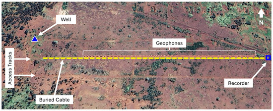
Figure 1.
Satellite image of the surface seismic data acquisition site.
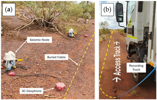
Figure 2.
Field images of the surface seismic data acquisition using co-located (a) seismic nodes with 3C geophones (b) and a buried fiber-optic cable.
The DAS surface seismic data was acquired using an existing fiber optic cable buried 10–15 cm deep and extending over 570 m along the access track. The fiber optic cable is a standard loose tube telecommunication cable. The cable was connected to a Fotech Theta interrogator powered by a generator on a trailer at the end of the track, further away from the drilling rig. The DAS data acquisition was conducted over two days only during the daytime due to operational restrictions on the overnight use of a diesel-powered generator.
The geophone surface seismic data was acquired using 128 tree-component (3C) geophones connected to battery-powered wireless nodes deployed on a 2D line along the buried cable with 3 m spacing between geophones. The geophones array recorded continuously over the same two-day period without any restrictions. The acquisition of 3C geophone data allowed the investigation of the horizontal-to-vertical spectral ratio (HVSR) technique to map the bedrock depth, which we do not discuss in this article. We limited subsequent analysis of the geophone data to the vertical component.
Table 1 below summarizes the timeline of the data acquisition in the context of surface seismic activity while drilling a 150 m depth borehole.

Table 1.
Data acquisition timeline of the passive surface seismic survey.
2.1. Surveying and Geometry
GPS surveying was performed for all the geophone locations and coordinates pre-loaded into the nodes before commencing the data recording to define accurate acquisition geometries after the deployment of geophone sensors. The geometry assignment was performed automatically into headers during the data acquisition as surveyed coordinates were pre-loaded into the nodes. Figure 3 shows a 2D map and a 3D view of the acquisition setup, the established geometries for the deployed sensors, and their relative locations to the drilled borehole.
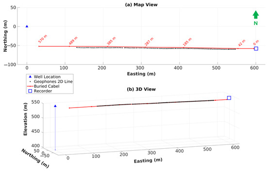
Figure 3.
Schematics showing (a) a 2D map and (b) a 3D view of the acquisition survey relative to the location of a 150-deep well.
As for the buried DAS cable, geometries were assigned based on tap tests upon connecting the interrogator to the fiber-optic cables and visual inspection of the recorded data. Figure 4 shows the color coding of channels of the surface DAS cable where the red color denotes unburied parts of the fiber-optic cable. The part of the cable usable for subsequent analysis is labeled in blue in Figure 4.
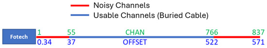
Figure 4.
Surface DAS geometry assignment.
2.2. Field Data Examples
2.2.1. Geophone Data Examples
The geophone dataset was harvested from all 132 wireless nodes in SEG-D format. The data were loaded using developed MATLAB scripts, and proper geometry was assigned after dividing it into 30 s chunks. The data were then converted to SEG-Y format for subsequent processing steps and visualized using the RadExPro software package. Figure 5a shows a zoomed view (nine hundred milliseconds) from five consecutive gathers of (30 s long) raw geophone data. Various seismic passive events were observed on the seismograms, related to traffic around drilling operations or a nearby highway. The recorded noise data is relatively broadband, starting from around 5 Hz and with a dominant frequency of around 17 Hz, as shown in Figure 5b.
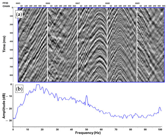
Figure 5.
(a) An example of traffic noise (a moving vehicle) on five consecutive surface geophone passive data field records with an overlay of a spectral analysis window in blue, and (b) their corresponding average amplitude spectrum over the indicated blue window.
2.2.2. DAS Data Examples
On the other hand, the DAS dataset was recorded by an interrogator in its native HDF5 format. Data were visualized using the RadExPro software package, which can read and handle the DAS data in native formats. Dedicated MATLAB scripts were developed to read the HDF5 files and then convert them to SEG-Y format for subsequent processing steps. The recorded passive surface seismic data is of reasonable quality, as shown in Figure 6. Figure 6a shows an example of surface passive data on DAS indicating noise from drilling the borehole, while Figure 6b shows some noise from an idling engine. Figure 6c shows the average amplitude spectra over the indicated colored windows in green and red. Both spectra show similar characteristics, with minimum frequencies around 7 Hz and peak frequencies around 22 Hz.
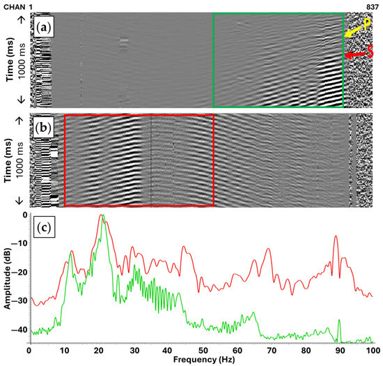
Figure 6.
An example of two different field records of the surface DAS passive data recorded (a) during drilling activities with the indicated green window used for spectral analysis where P-wave and S-wave can be identified as shown in yellow and red arrows, respectively, (b) toward the end of the recording when no drilling activities occurred (an idling engine) with an indicated red window for spectral analysis, and (c) the average amplitude spectra of the indicated colored windows.
3. Data Processing
Several pre-processing steps were applied to geophone and DAS data to conduct inversions for the shear wave velocities using multi-channel analysis of surface waves (MASW). We adapted the workflow described in [12,13]. For inversion, dispersion curves are required and they were computed after going through a data processing workflow. The workflow includes bandpass filtering, spectral whitening, cross-correlation to compute virtual sources, and stacking virtual source 30 s frames. Figure 7 shows the adapted workflow along with the main parameters used. Blue steps are common for geophone and DAS data, while magenta steps are unique for DAS.
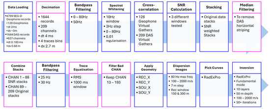
Figure 7.
The applied workflow for surface data processing and analysis. Blue steps are common for geophone and DAS data, while magenta steps are unique for DAS.
3.1. Geophone Data Preparation
We applied a 0–80 Hz bandpass filter before spectral whitening. Surface waves were not expected above 80 Hz. Additionally, we used a 50 Hz notch filter to remove machinery noise. Traces were spectrally balanced before cross-correlation. Balancing helps unify the input from different sources at different frequencies. Spectral whitening was computed in a 10 Hz window length with a 3 Hz window step. To create virtual source gathers, first, an interferometric approach was used by cross-correlating data of each geophone with every other one on the line. We correlated data in 30 s frames. To get virtual shots, causal (positive time lag) and acausal (negative time lag) were stacked together after the correlation. Selective signal-to-noise stacking was used to enhance data quality. Figure 8 shows examples of records after cross-correlation with channel 102 to form a virtual shot at this location.
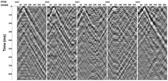
Figure 8.
An example of five different field records of the surface geophone passive data.
We investigated three different signal windows to enhance the virtual gathers and estimate the signal-to-noise ratio (SNR) for every cross-correlation frame for every virtual shot gather. Using the green signal window in Figure 9, the virtual gathers with better-than-average SNR were selected and normalized by their mean RMS amplitude level before stacking them.
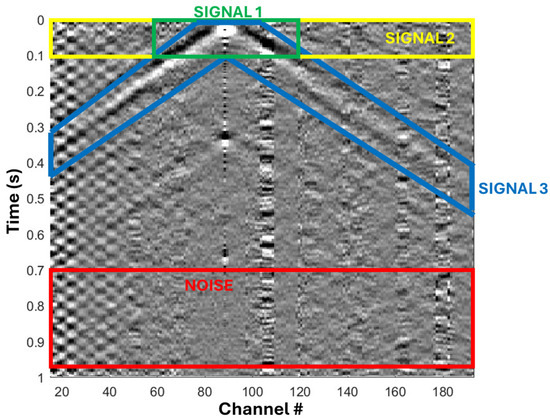
Figure 9.
Signal-to-noise calculation windows for selective stacking.
Figure 10 compares a virtual source gather before and after the SNR-weighted stacking. The SNR value has improved by five-fold, which is also reflected clearly in the virtual source gathers based on visual inspection.
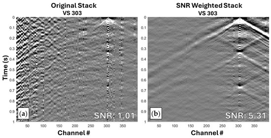
Figure 10.
A qualitative comparison for a geophone virtual source gather (a) before and (b) after SNR weighted stacking.
3.2. DAS Data Preparation
A similar workflow was applied to the surface DAS data. The surface DAS data have been down sampled to 4 ms and decimated spatially to 2.7 m spacing. Down sampling and decimation reduced the number of channels from 837 to 209, allowing for faster computation of subsequent steps. Bandpass and notch filtering were applied to the DAS data before spectral whitening and calculation of cross-correlations to generate virtual shot gathers.
Surface DAS data are noisier than geophone data; thus, selective signal-to-noise stacking enhances data quality. Using the green signal window in Figure 9, the virtual gathers with better-than-average SNR were selected and normalized by their mean RMS amplitude level before stacking them. After stacking, median filtering was applied to the stacked data to remove the common horizontal striping noise in the DAS data.
The resulting stacked virtual gathers varied in quality depending on the location on the 2D line. Selective signal-to-noise stacking was used to enhance data quality. The virtual gathers were then normalized by their mean RMS amplitude level before stacking them. Figure 11 compares four virtual source gathers on the 2D line at different locations. For virtual sources 22 and 88, located away from the drilling rig, SNR selective stacking generated satisfactory virtual source stacks. However, for virtual sources 95 and 180, located closer to the drilling rig, contrary to the original stacked virtual gathers, the SNR selective stacking did not produce better weighted stacks. Even though the SNR values indicate improvements after SNR-weighted stacking, visual inspection is required for confirmation, especially in cases where we lose signal continuity.
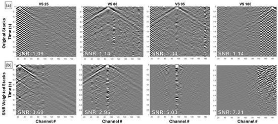
Figure 11.
A qualitative comparison for four different DAS virtual source gathers (a) before and (b) after SNR weighted stacking.
Virtual sources away from the rig (up to VS 25–88) were enhanced by SNR-weighted stacking, while virtual sources closer to the rig (VS 89–180) did not show any improvement after SNR-weighted stacking. The lack of signal improvement using SNR-weighted stacks for virtual gathers away from the drilling rig called for combining the data from the original and SNR-weighted stacks for subsequent data processing, as shown in Figure 12.
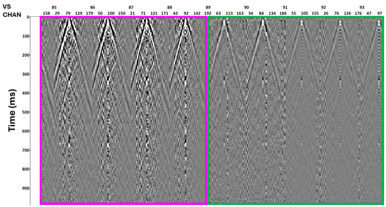
Figure 12.
The combined stacked DAS virtual source gathers, composed of the enhanced virtual sources (away from the rig), up to VS 88, as highlighted in magenta, and the remaining original virtual sources (closer to the rig), from VS 89 onward, as highlighted in green.
Virtual source gathers near drilling rig activities were contaminated by 30 Hz and 25 Hz mono-frequency noise from idling diesel engines and generators running at 1500–1800 rpm. The combined gathers were then equalized using the RMS amplitude to correct for different stack folds, as shown in Figure 13. After equalization, virtual source gathers corresponding to recording channels at both ends of the fiber-optic cable (channels 1–12 and 194–209), where the fiber cable is above the surface, were removed as they did not contain coherent signals due to poor coupling. The variable data quality demonstrates the importance of coupling for passive seismic surface wave analysis.
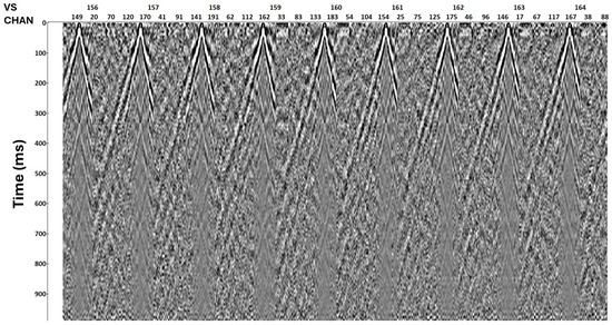
Figure 13.
A sample set of DAS virtual source gathers after mono-frequency filtering and trace equalization.
4. Data Analysis
4.1. Qualitative Analysis
4.1.1. Geophone Data Analysis
After preparing the passive geophone data, we look closely for amplitude anomalies in the data, such as strong noise or events. We computed an amplitude map for every acquisition day. We calculated a maximum absolute amplitude for every channel in a 30 s window. In this case, we limited the analysis to the vertical component of the geophone data for subsequent steps. The focus on the vertical component is due to the simplicity of processing workflows and the common use of one-component (1C) geophones for shallow subsurface surveys.
Figure 14 shows amplitude attribute sections computed for all surface geophones over the continuous recording period for each 30 s long record without gaps. Over nine hours during the first acquisition day, Figure 14a shows a detected linear event related to a fast-moving truck moving away from the well, marked by the magenta arrow. Shortly after that, closer to the well location, four major surface activities were recorded by many channels over one hour. This high amplitude noise (closer to the drilling pad) was related to the commencement of drilling operations on the first day. Much later in the evening, around 21:00, another linear event was detected, marked by the yellow arrow, of a fast-moving truck driving toward the well location. Figure 14b shows the continuation of the geophones recording on the second day and capturing the commencement of drilling on the second day around 09:00. Similar but stronger surface activities near the well location were detected. The cyan bars at the top of the plot mark periods of surface drilling activities, while magenta bars at the bottom mark periods of recording overlap with the DAS acquisition. The quiet period in the middle is the nighttime from 7 p.m. to 7 a.m. the next day.
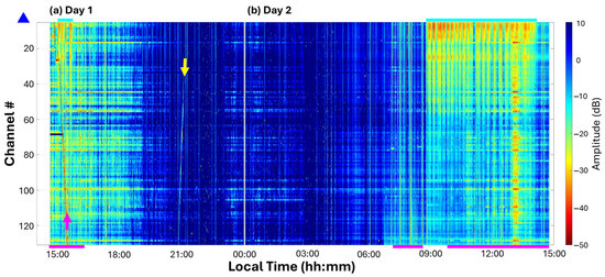
Figure 14.
Surface geophone data maximum absolute amplitude map of the (a) first day and (b) second day of continuous acquisition. The blue triangle marks the end of the 2D line closer to the well location. The magenta bars on the time scale denote recording periods overlapping with DAS acquisition, while cyan bars at the top mark periods of drilling surface activities. The magenta and yellow arrows mark instances where moving vehicles were detected along the 2D line, moving away and toward the drilling rig, respectively.
4.1.2. DAS Data Analysis
Similarly, after preparing the passive DAS data, we looked closely for amplitude anomalies in the data. We computed an amplitude map for every acquisition day to handle a large volume of accumulated data from the DAS. We calculated a maximum absolute amplitude for every channel in a 30 s window.
Figure 15 shows the amplitude attribute sections computed for all surface DAS channels over the whole recording period for each 30 s long record, with a couple of gaps in the DAS data recording. The first gap was due to daylight restriction, and the second was due to field issues encountered. Relative to the geophones nodal acquisition, the DAS data acquisition started four hours before and ended an hour and a half after. The high amplitude noise at the two ends of the fiber-optic cable is worth noting as they are above the surface. Over five hours during the first day of acquisition, Figure 15a shows some detected events that were related to a slow-moving truck and human activities heading toward the well location, marked by the blue arrow, during the deployment of surface wireless geophone nodes along the same track where the fiber-optic cable is buried. We can also see a faint hit of the fast-moving truck moving away from the well, marked by the magenta arrow, which was also identified on the geophone data. Shortly after that, closer to the well location, four major surface activities were recorded by many channels over one hour. This high amplitude noise (closer to the drilling pad) is related to the commencement of drilling operations on the first day. Figure 15b shows the commencement of the DAS recording on the second day, followed by a gap of an hour, during which drilling commenced for the second day. Similar surface activities near the well location were detected, followed by a fast-moving vehicle heading further from the well location, marked by a blue arrow. The cyan bars at the top of the plot mark periods of surface drilling activities, while magenta bars at the bottom mark periods of recording overlaps with the geophone acquisition.
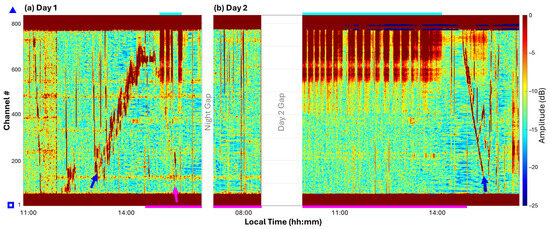
Figure 15.
Surface DAS data maximum absolute amplitude section of the (a) first and (b) second acquisition days, highlighting a couple of recording gaps. The blue square marks the location of the DAS interrogator by channel 1, and the blue triangle marks the end of the cable closer to the well location. The magenta bars on the time scale denote recording periods overlapping with the geophone array, while cyan bars at the top mark periods of drilling surface activities. The magenta arrow indicates the same moving vehicle heading away from the rig as detected at the start of geophone recording. The blue arrows mark a detected slow-moving vehicle along the 2D line during the geophone node deployment on the first day heading toward the drilling rig and a fast-moving vehicle moving away from the rig on the second day.
4.2. Comparisons
One of the main challenges of running a passive seismic survey at this site was purely operational. Due to nighttime restrictions, the collocated geophone array and DAS cable covered different periods of passive recording, with overlaps during the daytime. As such, our comparisons focused on one example from the first day of recording, where surface drilling activities were taking place, and the resulting seismic responses were recorded simultaneously by geophones and DAS.
Figure 16 shows two raw seismograms of three seconds in length recorded on day one at 15:33:30. The left side of these seismograms is closer to the drilling rig. Figure 17 shows the spectra computed for the corresponding color-coded windows in Figure 16. While recorded using two different special sampling rates, both seismograms cover the same 380 m distance profile. The raw seismograms show the same seismic event recorded by geophones and DAS, where P-wave and S-wave reflections can easily be recognized on both records. Horizontal striping is prominent at around two thousand milliseconds on the DAS data. Additionally, the 12 m gauge length caused smearing of the recorded reflections on the DAS data and made them look cleaner.
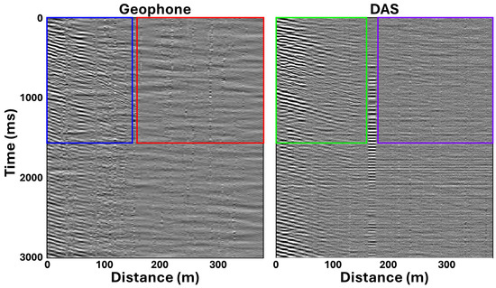
Figure 16.
A comparison between geophone and DAS recordings of the same event on day one at 15:33:30, with color-coded spectral analysis windows. The colored windows indicate where spectra were computed for comparisons. The blue and green windows represent the average amplitude spectra for drilling activity near the rig for geophone and DAS data, respectively. Similarly, the red and purple windows represent the spectra computed farther from the rig for geophone and DAS data, respectively.
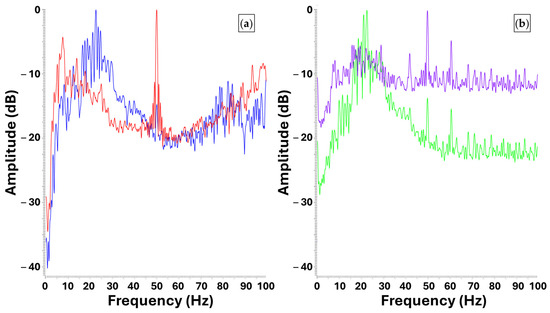
Figure 17.
Amplitude spectra for the color-coded windows in Figure 16, (a) where blue and red amplitude spectra are for drilling activity near and away from the rig for geophone data, respectively. (b) While the green and purple amplitude spectra are for DAS channels near and away from the rig, respectively.
On the other hand, the geophone data are contaminated by spikes of higher frequencies, as each channel was recorded by a single geophone without any array forming, which is evident in the spectra in Figure 17a. The spectra also show a clear 50 Hz mono-frequency on both the geophone and DAS data. However, 60 Hz mono-frequency noise appears only on the DAS data purple and green spectra.
The data used in this comparison were not used in the subsequent MASW workflow as they were contaminated by surface drilling activities around the drilling rig, limiting their frequency bandwidths, as shown in the blue and green spectra in Figure 17. This is explained further in the following subsection but by using computed dispersion curves. The red and purple spectra show different geophone and DAS data responses away from the drilling rig, with a noticeably flat DAS spectrum.
4.3. Dispersion Curves
Also known as spectral analysis of surface waves (SASW), this provides good horizontal resolution but comes with challenges, such as its susceptibility to coherent noise and the variable coupling of seismic sensors. On the other hand, MASW is a robust method [9], but it lacks horizontal resolution. Hence, we adapted the stacking of surface waves (SSW) method described in [33] to compute better quality and higher horizontal resolution dispersion images.
4.3.1. Geophone Data
We calculated dispersion images with a seven-meter step for the vertical component geophone data, phase velocity ranges from 100 to 2000 m/s, and frequency ranges from 0 to 80 Hz. We computed the images with a 300 m maximum offset window for frequencies below 15 Hz to improve phase velocity resolution. We used a smaller window of 150 m for frequencies above 15 Hz to improve spatial resolution. Dispersion images were computed for all the data, including drilling and non-drilling periods, and for data without drilling. RadExPro software was used to pick the dispersion curves manually.
To understand the drilling noise contribution for the experiment geometry, we compared the resulting virtual shot gathers obtained using all data with those computed excluding drilling time, as shown in Figure 18a,b. Excluding the drilling periods yielded less contaminated gathers. This is attributed to the recording of strong energy drilling noise, especially on closer geophones, which affects the low-frequency part of the spectrum, as is evident in the first two virtual gathers on the left of Figure 18a. Also, stacking several virtual shot gathers in a running window was applied to increase the signal-to-noise ratio of the dispersion images, as shown in Figure 18b.
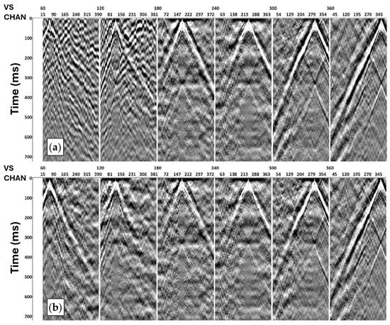
Figure 18.
A comparison of virtual shot gathers computed for (a) all data and (b) data excluding the time of the active drilling.
Figure 19 shows examples of dispersion images at the rig’s close and far proximity. The top panels of Figure 19a,b show limited frequency bandwidth compared to the bottom panels of Figure 19c,d. Images without drilling have better resolution at low frequencies, as shown in Figure 19b,d, which provides better inversion stability at deeper depths.
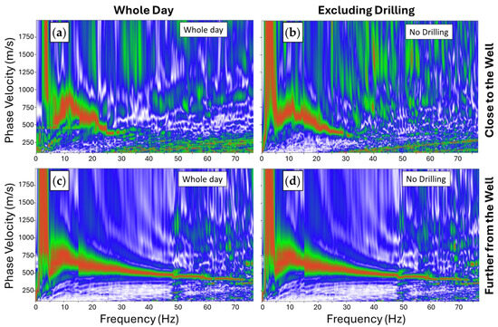
Figure 19.
Dispersion images for channels close to the rig (top panels) vs. channels away from the rig (bottom panels). Images (a,c) were calculated from geophone data at all times, while (b,d) were from data excluding drilling time.
4.3.2. DAS Data
Dispersion images were computed for all the virtual source gathers, as shown in Figure 20. Due to the daytime restriction for DAS acquisition, the recorded data are contaminated with noise due to the drilling surface activities. A couple more things need to be noted when comparing DAS dispersion images with those computed on the surface geophone vertical component data. First, they are of poor quality, even worse than the geophone dispersion images closer to the rig. They also have limited bandwidths ranging from 8 to 26 Hz, which are not adequate to generate a reliable model in depth. Second, they have a lower resolution in the vertical velocity axes, especially at lower frequencies, making them unusable for further analysis. This also provides a better understanding for future passive DAS data acquisitions.
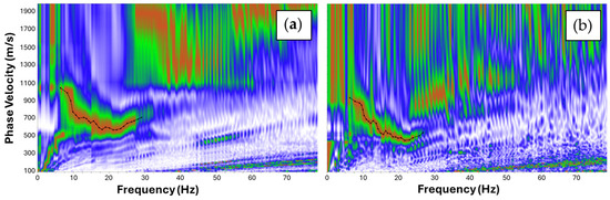
Figure 20.
Dispersion images from two different DAS virtual source gathers from (a) the beginning of the DAS 2D line (further from the well) and (b) the end of the DAS 2D line (closer to the well).
The resulting dispersion images from the DAS data are quite narrow-banded due to the nature of the DAS measurements at a certain gauge length. As the average shear wave velocity of the near-surface in the area is about 500 m/s, the recording parameter of around 12 m gauge length results in resolving frequencies without aliasing of up to 40–50 Hz. The Fotech Theta interrogator has good sensitivity but has internal filters in the low frequency band.
4.4. Inversion (MASW)
In the final step of the workflow, the fundamental modes of all dispersion curves were picked manually and then inverted using Occam’s inversion implementation to minimize the root-mean-squared error between computed curves for different virtual sources while maintaining model smoothness, which results in a 2D S-wave velocity profile. At this stage, the inversion was run separately for continuous recording at all times and for recordings excluding drilling for the geophone data.
The maximum wavelength is the main parameter controlling the maximum depth of the resulting model, which is usually . The maximum wavelengths were different for each of the two cases, as detailed further below. On the other hand, the minimum wavelength controls the minimum depth of the model above, for which we may not have reliable velocity information corresponding to shallow layers. In both cases, the maximum frequencies are around 73 Hz, corresponding to an equivalent wavelength of around 13.7 m.
Figure 21a shows the shear wave velocity profile obtained using dispersion curves computed for geophone data recorded at all times. In this case, the minimum frequency is around 7 Hz, equivalent to a wavelength of 143 m. The resulting inverted model is expected to have a maximum depth of around seventy-one meters. Even though Figure 21a shows a model that extends up to 100 m in depth, inverted velocities below 60 m are of low confidence. Yellow arrows highlight regions where inversion is unstable due to poor resolution at low frequencies and the noise from surface drilling activities.
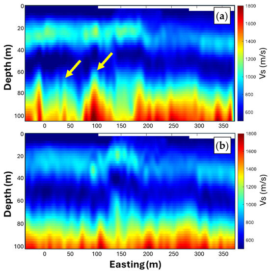
Figure 21.
Shear wave velocity profiles obtained (a) for all data where yellow arrows highlight areas of unstable inversion, (b) for data without drilling noise.
Figure 21b shows the shear wave velocity profile obtained using dispersion curves computed for geophone data without drilling noise. The results are much more consistent, especially at larger depths, due to better resolution at lower frequencies. In this case, the minimum frequency is around 5 Hz, equivalent to a wavelength of two hundred meters. The resulting inverted model is expected to have a maximum depth of around one hundred meters.
Downhole gamma logging tools are commonly used to measure subsurface layer rocks’ naturally occurring radioactivity, including elements such as potassium, radon, uranium and thorium. As such, different rock types would yield different intensities of measured gamma rays. The relative radioactivity of rocks is then used as an in-hole tool to map the stratigraphy of the subsurface [34]. Figure 22 visualizes the second result of the near-surface shear wave velocity model with an overlay of a gamma-log from a well of 65 m depth close to the middle of the 2D line, showing an excellent correlation of the gamma-log with the velocity trend. The correlation is clearly observed in the high-intensity gamma values for the low-velocity shallow layer, with an estimated four hundred meters per second velocity. Similarly, the gamma-log shows a high intensity for the deeper layer at around fifty meters, with an estimated velocity of 550 m per second. The intensity of the gamma-log decreased for the sandwiched layer between 12 to 50 m, which had a higher velocity of around eight hundred meters per second. A visual validation could not be made for depths larger than 65 m, where we do not have gamma-log measurements. This interpretation is consistent with other geological interpretations in the same region where gamma-logs show signatures of the Joffre, Whaleback Shale and Dale Gorge Members as previously interpreted by Kerr [35].
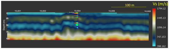
Figure 22.
Near-surface shear wave velocity (Vs) model with an overlay of gamma-log.
5. Discussion
5.1. Data Acquisition Considerations
Deploying a large array using fiber-optic cables and nodes is quite efficient. However, the 2D geometry did not allow for capturing the passive energy of sources from various azimuths. A 3D configuration of the sensor array geometries would be optimal to account for the direction of the energy arrivals. Cross-type sensor spreads with an array oriented at different azimuths can be considered for future surveys.
Any knowledge of passive energy sources such highways, mines, railways, and drilling should be considered in the design of passive surveys to orient the array optimally. An extended recording time of about twenty-four hours is helpful to obtain low-frequency data and cover different times of the day, focusing on various ambient noise patterns. A longer recording time is preferable to enhance the data quality and provide higher signal-to-noise ratios.
The choice of the DAS interrogator can significantly affect data quality. Two considerations must be taken when designing a passive seismic survey using DAS. First, using an interrogator capable of recording low and ultra-low frequency data, around and less than 1 Hz, is beneficial in reconstructing shear wave velocity profiles to achieve deeper model depths. Additionally, prior knowledge of the velocities should be considered to select suitable DAS recording parameters, such as gauge length and pulse length, to optimize the balance between signal-to-noise and resolution at high frequencies.
5.2. The Workflow
This article adopted a cross-correlations processing workflow to retrieve virtual shot gathers containing information about surface waves from long passive seismic records. These virtual gathers were then improved using spectral whitening and stacking before manually picking the fundamental mode and inverting them. MASW mainly lacks horizontal resolution due to the averaging of different wavelength components of surface waves, so it is worth looking at better ways to optimize the resolution [36].
6. Conclusions
A passive seismic survey was successfully conducted at a mineral exploration site in the Pilbara region of Western Australia. The survey collected passive seismic data using 3C geophones connected to nodes and a surface-buried fiber-optic cable co-located in a 2D array geometry. Passive data recordings were collected over two days. Geophone node recordings were acquired continuously and extended overnight, while DAS recordings were only acquired during daylight. A one-day delay in the commencement of drilling of the well allowed for the collection of more passive data during nighttime using the surface geophones, which provided valuable insight into the use of passive data and passive interferometric techniques in the presence of drilling noise. The recordings were just enough to assess the MASW workflow on both recordings. However, the lack of DAS recordings during nighttime did not allow for representative comparisons of data and inverted models, whereas geophone recordings resulted in satisfactory models. The dissatisfactory results from the DAS recordings do not imply that DAS cannot be used for MASW but rather provide insights into improving the application in future experiments. Noise created by drill rigs during active operations is coherent and narrow-banded for the surface wave analysis. It is mainly dominated by monotonous signals from the diesel engines, which affects the spectral analysis of surface waves, leading us to focus on data recorded, excluding drilling activities and using stacking to improve results [33].
The shear wave velocity models were reconstructed up to a depth of one hundred meters using geophone data acquired during the quiet nighttime period. The obtained S-wave velocity (Vs) model, using surface geophones, correlated well with the log data from a borehole in the middle of the 2D line. In summary, the complete workflow for MASW has been successfully demonstrated, starting with the data acquisition, processing, computation of dispersion curves, and then inverting for the shear wave velocity profiles. The assessment study showed the value of passive seismic data for subsurface characterization and the potential for further development and improvements.
Author Contributions
Conceptualization, K.T., R.I. and E.A.-H.; methodology, R.I. and E.A.-H.; software, R.P., R.I., E.A.-H.; validation, R.I. and E.A.-H.; formal analysis, R.I. and E.A.-H.; investigation, R.I. and E.A.-H.; resources, R.P. and K.T.; data curation, K.T. and P.S.; writing—original draft preparation, E.A.-H.; writing—review and editing, E.A.-H., R.I., K.T., P.S. and R.P.; visualization, E.A.-H. and R.I.; supervision, K.T. and R.P.; project administration, K.T.; funding acquisition, K.T. All authors have read and agreed to the published version of the manuscript.
Funding
This case study has been supported by the Mineral Exploration Cooperative Research Centre (MinEx CRC), whose activities are funded by the Australian Government’s Cooperative Research Centre Program. This is MinEx CRC document 2025/04.
Data Availability Statement
Restrictions apply to the availability of these data. Data were obtained from BHP and are available from the corresponding author with BHP’s permission.
Acknowledgments
The authors would like to thank Ashley Grant and Nathan Tabain from BHP for their support during the data acquisition campaign and permission to publish the data. We would also like to thank Dominic Howman and Murray Hehir for their assistance with the data acquisition.
Conflicts of Interest
The authors declare no conflicts of interest.
References
- Latham, G.V.; Ewing, M.; Press, F.; Sutton, G.; Dorman, J.; Nakamura, Y.; Toksöz, N.; Wiggins, R.; Derr, J.; Duennebier, F. Passive Seismic Experiment. Science 1970, 167, 455–457. [Google Scholar] [CrossRef]
- Dal Moro, G.; Pipan, M.; Forte, E.; Finetti, I. Determination of Rayleigh Wave Dispersion Curves for near Surface Applications in Unconsolidated Sediments. In Proceedings of the SEG Technical Program Expanded Abstracts 2003, Dallas, TX, USA, 26–31 October 2003; Society of Exploration Geophysicists: Houston, TX, USA, 2003; pp. 1247–1250. [Google Scholar]
- Asten, M.W. Passive Seismic Methods Using the Microtremor Wave Field. ASEG Ext. Abstr. 2004, 2004, 1–4. [Google Scholar] [CrossRef]
- Duncan, P.M. Is There a Future for Passive Seismic? First Break 2005, 23, 111–115. [Google Scholar] [CrossRef]
- Artman, B. Imaging Passive Seismic Data. Geophysics 2006, 71, SI177–SI187. [Google Scholar] [CrossRef]
- Artman, B. Passive Seismic Imaging; Stanford University: Stanford, CA, USA, 2007. [Google Scholar]
- Ivanov, J.; Leitner, B.; Shefchik, W.; Shwenk, J.T.; Peterie, S.L. Evaluating Hazards at Salt Cavern Sites Using Multichannel Analysis of Surface Waves. Lead. Edge 2013, 32, 298–305. [Google Scholar] [CrossRef][Green Version]
- Curtis, A.; Gerstoft, P.; Sato, H.; Snieder, R.; Wapenaar, K. Seismic Interferometry—Turning Noise into Signal. Lead. Edge 2006, 25, 1082–1092. [Google Scholar] [CrossRef]
- Park, C.B.; Miller, R.D.; Xia, J. Multichannel Analysis of Surface Waves. Geophysics 1999, 64, 800–808. [Google Scholar] [CrossRef]
- Park, C.B.; Miller, R.D.; Xia, J.; Ivanov, J. Multichannel Analysis of Surface Waves (MASW)—Active and Passive Methods. Lead. Edge 2007, 26, 60–64. [Google Scholar] [CrossRef]
- Miller, R.; Xia, J.; Park, C.B.; Ivanov, J.M. The History of MASW. Lead. Edge 2008, 27, 568. [Google Scholar] [CrossRef]
- Cheng, F.; Xia, J.; Xu, Y.; Xu, Z.; Pan, Y. A New Passive Seismic Method Based on Seismic Interferometry and Multichannel Analysis of Surface Waves. J. Appl. Geophys. 2015, 117, 126–135. [Google Scholar] [CrossRef]
- Cheng, F.; Xia, J.; Luo, Y.; Xu, Z.; Wang, L.; Shen, C.; Liu, R.; Pan, Y.; Mi, B.; Hu, Y. Multichannel Analysis of Passive Surface Waves Based on Cross-correlations. Geophysics 2016, 81, EN57–EN66. [Google Scholar] [CrossRef]
- Morton, S.L.; Ivanov, J.; Peterie, S.L.; Miller, R.D.; Livers-Douglas, A.J. Passive Multichannel Analysis of Surface Waves Using 1D and 2D Receiver Arrays. Geophysics 2021, 86, EN63–EN75. [Google Scholar] [CrossRef]
- Miller, R.D.; Xia, J.; Park, C.B.; Ivanov, J.M. Multichannel Analysis of Surface Waves to Map Bedrock. Lead. Edge 1999, 18, 1392–1396. [Google Scholar] [CrossRef]
- Park, C.B.; Miller, R.D.; Ryden, N.; Xia, J.; Ivanov, J. Combined Use of Active and Passive Surface Waves. JEEG 2005, 10, 323–334. [Google Scholar] [CrossRef]
- Da Col, F.; Papadopoulou, M.; Koivisto, E.; Sito, Ł.; Savolainen, M.; Socco, L.V. Application of Surface-Wave Tomography to Mineral Exploration: A Case Study from Siilinjärvi, Finland. Geophys. Prospect. 2020, 68, 254–269. [Google Scholar] [CrossRef]
- Glubokovskikh, S.; Pevzner, R.; Sidenko, E.; Tertyshnikov, K.; Gurevich, B.; Shatalin, S.; Slunyaev, A.; Pelinovsky, E. Downhole Distributed Acoustic Sensing Provides Insights Into the Structure of Short-Period Ocean-Generated Seismic Wavefield. J. Geophys. Res. Solid Earth 2021, 126, e2020JB021463. [Google Scholar] [CrossRef]
- Ajo-Franklin, J.B.; Dou, S.; Lindsey, N.J.; Monga, I.; Tracy, C.; Robertson, M.; Tribaldos, V.R.; Ulrich, C.; Freifeld, B.; Daley, T.; et al. Distributed Acoustic Sensing Using Dark Fiber for Near-Surface Characterization and Broadband Seismic Event Detection. Sci. Rep. 2019, 9, 1328. [Google Scholar] [CrossRef]
- Fang, G.; Li, Y.E.; Zhao, Y.; Martin, E.R. Urban Near-Surface Seismic Monitoring Using Distributed Acoustic Sensing. Geophys. Res. Lett. 2020, 47, e2019GL086115. [Google Scholar] [CrossRef]
- Ziramov, S.; Bona, A.; Tertyshnikov, K.; Pevzner, R.; Urosevic, M. Application of 3D Optical Fibre Reflection Seismic in Challenging Surface Conditions. First Break 2022, 40, 79–89. [Google Scholar] [CrossRef]
- Meneghini, F.; Poletto, F.; Bellezza, C.; Farina, B.; Draganov, D.; Van Otten, G.; Stork, A.L.; Böhm, G.; Schleifer, A.; Janssen, M.; et al. Feasibility Study and Results from a Baseline Multi-Tool Active Seismic Acquisition for CO2 Monitoring at the Hellisheiði Geothermal Field. Sustainability 2024, 16, 7640. [Google Scholar] [CrossRef]
- Lim Chen Ning, I.; Sava, P. Multicomponent Distributed Acoustic Sensing: Concept and Theory. Geophysics 2018, 83, P1–P8. [Google Scholar] [CrossRef]
- Innanen, K.A.; Lawton, D.; Hall, K.; Bertram, K.L.; Bertram, M.B.; Bland, H.C. Design and Deployment of a Prototype Multicomponent Distributed Acoustic Sensing Loop Array. In Proceedings of the SEG Technical Program Expanded Abstracts 2019, San Antonio, TX, USA, 15–20 September 2019; Society of Exploration Geophysicists: Houston, TX, USA, 2019; pp. 953–957. [Google Scholar]
- Daley, T.M.; Freifeld, B.M.; Ajo-Franklin, J.; Dou, S.; Pevzner, R.; Shulakova, V.; Kashikar, S.; Miller, D.E.; Goetz, J.; Henninges, J.; et al. Field Testing of Fiber-Optic Distributed Acoustic Sensing (DAS) for Subsurface Seismic Monitoring. Lead. Edge 2013, 32, 699–706. [Google Scholar] [CrossRef]
- Bakulin, A.; Silvestrov, I.; Pevzner, R. Surface Seismic with DAS: Looking Deep and Shallow at the Same Time. In Proceedings of the SEG Technical Program Expanded Abstracts 2018, Anaheim, CA, USA, 14–19 October 2018; Society of Exploration Geophysicists: Houston, TX, USA, 2018; p. 20. [Google Scholar]
- Bakulin, A.; Silvestrov, I.; Pevzner, R. Surface Seismics with DAS: An Emerging Alternative to Modern Point-Sensor Acquisition. Lead. Edge 2020, 39, 808–818. [Google Scholar] [CrossRef]
- Mellors, R.; Trabant, C. DAS Data Management Challenges and Needs; European Geosciences Union (EGU): Vienna, Austria, 2022; p. EGU22-6573. [Google Scholar]
- Rix, G.; Stokoe, K.; Roesset, J. Experimental Study of Factors Affecting the Spectral-Analysis-of-Surface-Waves Method. Interim Report; Center for Transportation Research Library, The University of Texas at Austin: Austin, TX, USA, 1991. [Google Scholar]
- Park, C.; Miller, R.; Laflen, D.; Neb, C.; Ivanov, J.; Bennett, B.; Huggins, R. Imaging Dispersion Curves of Passive Surface Waves. In Proceedings of the SEG Technical Program Expanded Abstracts 2004, Denver, CO, USA, 10–15 October 2004; Society of Exploration Geophysicists: Houston, TX, USA, 2004; pp. 1357–1360. [Google Scholar]
- Xia, J.; Miller, R.D.; Park, C.B. Estimation of Near-surface Shear-wave Velocity by Inversion of Rayleigh Waves. Geophysics 1999, 64, 691–700. [Google Scholar] [CrossRef]
- Constable, S.C.; Parker, R.L.; Constable, C.G. Occam’s Inversion: A Practical Algorithm for Generating Smooth Models from Electromagnetic Sounding Data. Geophysics 1987, 52, 289–300. [Google Scholar] [CrossRef]
- Neducza, B. Stacking of Surface Waves. Geophysics 2007, 72, V51–V58. [Google Scholar] [CrossRef]
- Russell, W.L. The Total Gamma Ray Activity of Sedimentary Rocks as Indicated by Geiger Counter Determinations. Geophysics 1944, 9, 180–216. [Google Scholar] [CrossRef]
- Kerr, T.L.; O’Sullivan, A.P.; Podmore, D.C.; Turner, R.; Waters, P. IRON: Geophysics and Iron Ore Exploration: Examples from the Jimblebar and Shay Gap-Yarrie Regions, Western Australia. ASEG Ext. Abstr. 1994, 1994, 355–368. [Google Scholar] [CrossRef]
- Ivanov, J.; Xia, J.; Miller, R.D. Optimizing Horizontal-Resolution Improvement of the MASW Method. In Proceedings of the Symposium on the Application of Geophysics to Engineering and Environmental Problems, Seattle, WA, USA, 2–6 April 2006; Environment and Engineering Geophysical Society: Denver, CO, USA, 2006; pp. 1128–1134. [Google Scholar]
Disclaimer/Publisher’s Note: The statements, opinions and data contained in all publications are solely those of the individual author(s) and contributor(s) and not of MDPI and/or the editor(s). MDPI and/or the editor(s) disclaim responsibility for any injury to people or property resulting from any ideas, methods, instructions or products referred to in the content. |
© 2025 by the authors. Licensee MDPI, Basel, Switzerland. This article is an open access article distributed under the terms and conditions of the Creative Commons Attribution (CC BY) license (https://creativecommons.org/licenses/by/4.0/).