Fine-Scale Stratigraphic Identification Using Machine Learning Trained on Multi-Site CPTU Data

Abstract

The piezocone penetration test (CPTU) provides rapid, continuous measurements of in situ geotechnical parameters, making it a valuable tool for soil classification and stratigraphic identification. However, conventional classification methods frequently exhibit poor cross-regional generalizability and remain limited in achieving fine-grained stratigraphic identification. To address these limitations, this study constructs a cross-regional CPTU soil classification dataset by integrating data from three sources: the Premstaller Geotechnik database, the Global-CPT/3/1196 database, and a Chinese engineering project database. The compiled dataset was subsequently partitioned into a training set of 454,184 samples and three independent test sets. Three feature combinations and four machine learning algorithms—Support Vector Machine (SVM), K-Nearest Neighbors (KNN), Artificial Neural Network (ANN), and Extreme Gradient Boosting (XGBoost), were evaluated in terms of classification performance and cross-regional robustness. Results indicate that the XGBoost-based model, using Depth, corrected cone resistance (q_t), friction ratio (R_f), pore pressure ratio (B_q), normalized friction ratio (F_r), and pore pressure (u₂) as inputs, achieved the highest performance across the three independent test sets. Misclassifications primarily occurred between adjacent soil types with similar physical characteristics. SHapley Additive exPlanations (SHAP) analysis indicated that F_r and q_t were the dominant contributors to model predictions; R_f played an important role in minority classes; Depth showed relatively balanced importance across classes, while B_q and u₂ made minimal contributions. Applying the best-performing model to unseen CPTU data and comparing the predictions with borehole logs showed that the model not only preserves overall stratigraphic trends but also identifies finer-scale stratigraphic details.

1. Introduction

For many years, the piezocone penetration test (CPTU) has been an efficient and widely used in situ method in geotechnical engineering. CPTU provides continuous, real-time measurements of key parameters—cone tip resistance (q_c), sleeve friction (f_s), and pore pressure (u₂), thereby greatly reducing the need for soil sampling and providing essential data for soil classification and geotechnical characterization.

In soil classification, chart-based methods are still the most common empirical approach. These methods classify soils by mapping CPTU measurements onto designated regions of two-dimensional classification charts. Early charts primarily relied on raw parameters such as q_c, f_s [1,2,3,4]. Subsequently, some studies proposed the importance of u₂, normalized cone resistance (Q_t), and normalized friction ratio (F_r) in distinguishing fine-grained soils and those near classification boundaries [5]. Other studies have introduced the soil behavior type index (I_c) as a numerical index to simplify soil classification from CPTU data [6]. However, these methods have limited ability to distinguish soil behavior in transitional soils where partial consolidation prevails [7]. Later, CPTU-based soil classification was revised into a behavior-based system that highlights soil response to stress–strain conditions, including contractive or dilative tendencies, sensitivity, and microstructural effects [8]. To address limitations in marine sediment studies, a triangular chart was introduced to classify sediments into seven types [9]. Although these approaches offer improved applicability and interpretability, they still struggle in areas of complex stratigraphy or transitional boundaries.

In recent years, machine learning methods based on CPTU data have been widely studied owing to their capability of handling large-scale, nonlinear data. Among them, clustering algorithms have been employed to detect intrinsic correlations within the data and thereby delineate soil strata and transitional boundaries [10,11,12,13,14,15,16]. Probabilistic models, typically grounded in statistical theory and inference, provide a framework in which results and predictions can be expressed and interpreted in terms of probability [17,18,19,20,21,22,23,24]. Neural networks, inspired by the information transfer and processing mechanisms of biological neurons, have been employed to capture complex subsurface features and patterns [25,26,27,28,29,30,31]. Since single models are limited in handling complex data, researchers have attempted different types of models, such as Support Vector Machine (SVM), K-Nearest Neighbors (KNN), and Decision Tree (DT), among others, to evaluate performance differences [32,33,34,35,36,37]. Some studies have employed various optimization strategies and ensemble machine learning approaches to enhance classification accuracy and model stability [38,39,40,41,42]. However, these studies often rely on data from a single site or region for model training. While this approach allows evaluation on local datasets, it can overestimate the model’s generalization to new areas because training and test samples may be spatially proximate or otherwise non-independent.

To address the limitations of existing studies, this study develops a machine learning model for soil classification based on a cross-regional CPTU dataset, aiming for robust generalization performance. The training set spans multiple countries and regions, comprising 454,184 samples. Model generalizability is evaluated on three independent test sets geographically distant from the training data. Four machine learning algorithms are compared across three feature combinations, with Balanced accuracy, F₁-weighted, and Cohen’s Kappa used as evaluation metrics. In addition, the SHapley Additive exPlanations (SHAP) method is employed to interpret the best-performing model, which is then applied to unseen CPTU data for stratigraphic prediction to assess its engineering applicability.

2. Methodologies

This study develops a soil classification model based on machine learning and CPTU data, with the framework overview presented in Figure 1. Model development proceeds in four steps. First, CPTU data are preprocessed and partitioned into a training set and independent test sets. Second, multiple machine learning models are trained on the training set, with hyperparameters optimized using 5-fold cross-validation to identify the optimal model configuration. Third, the generalization performance of the trained models is rigorously evaluated on the independent test sets. Finally, the best-performing model is deployed to predict stratigraphy on entirely unseen CPTU data. This framework ensures a clear separation between data preparation, training, validation, evaluation, and prediction, thereby enforcing rigorous and reproducible model development.

2.1. CPTU Dataset

The dataset was compiled from the Premstaller Geotechnik database, the Global-CPT/3/1196 database, and a CPTU database from a Chinese engineering project, covering multiple countries and regions. After data cleaning, 491,781 valid samples remained (all subsequent data refer to post-cleaning results).

Table 1. Summary of CPTU data sources and descriptive statistics compiled into the study dataset (soundings, samples, depth ranges, and mean parameter values).

Database	Country	Site	Soundings	Samples	Depth Range (m)	Mean qc (MPa)	Mean fs (kPa)	Mean u2 (kPa)
Premstaller Geotechnik	Austria	Salzburg Basin	30	67,787	0.01–40.01	7.45	51.97	300.15
		Salzach Valley	1	1319	0.01–13.90	15.68	121.62	41.70
		Zell Basin	27	67,892	0.01–49.94	3.49	36.56	129.12
		Grossarl Valley	3	3218	0.01–16.84	10.26	355.11	6.45
		Flachgau	11	11,382	0.01–20.68	4.54	85.91	54.99
		Enns Valley	8	10,844	0.01–44.94	7.91	53.84	133.44
		Mondsee Basin	3	1531	0.12–7.33	3.53	67.42	11.98
Global- CPT/3/1196	New Zealand	Marshland	24	22,562	0.01–15.00	7.51	47.86	−17.87
		Tauranga	28	66,945	0.01–32.89	6.43	92.79	97.62
		Hastings	13	32,500	0.50–30.80	6.87	62.73	145.45
		Richmond	13	10,513	0.01–9.69	5.34	208.91	−33.09
		Port Nelson	27	10,659	0.01–14.00	4.88	53.18	5.58
		Whangārei	30	21,047	0.01–14.96	3.26	88.99	135.04
		Lower Hutt	29	28,153	0.01–9.90	14.91	106.85	−39.73
	The Netherlands	Leiden	29	33,773	0.31–12.29	0.41	14.02	75.59
	USA	Baytown	9	3862	0.02–15.34	2.23	90.43	−2.38
		Hollywood	25	16,425	0.02–13.62	5.23	45.86	85.68
		Missouri	7	2526	0.05–24.05	7.77	329.20	23.68
	Italy	Bologna	34	38,844	0.04–35.30	2.18	81.31	304.09
	Japan	Oda River	25	1780	0.05–10.90	4.35	34.79	18.09
	China	Suqian	10	4016	0.05–22.15	5.27	65.15	52.28
Chinese engineering project	China	Shanghai	5	34,203	4.45–69.88	9.72	38.57	534.18
Total			391	491,781

summarizes the CPTU data sources, number of soundings, sample counts, depth ranges, and the mean values of each parameter.

The Premstaller Geotechnik database, compiled by Oberhollenzer et al., contains extensive in situ test data collected by Premstaller Geotechnik ZT GmbH in Austria and Germany, including the cone penetration test (CPT) and CPTU records [43]. This study selected several basin and valley sites in Austria (Salzburg Basin, Zell Basin, Salzach Valley, Grossarl Valley, Flachgau, Enns Valley, and Mondsee Basin), comprising 83 CPTU soundings and yielding 163,973 samples. The sampling locations cover two types of depositional environments: basin areas, characterized by high sedimentation rates, thick stratigraphic sequences, predominantly fine-grained deposits, and distinct bedding; and valley areas, influenced by glacial processes and primarily composed of gravel–sand–silt mixtures. This database represents a typical glacial–basin–valley depositional system and provides sufficient regional representation. CPTU measurements were conducted using a standard cone with a cross-sectional area of 15 cm² at a constant penetration rate of 2 cm/s.

The Global-CPT/3/1196 database was compiled by the ISSMGE Technical Committee TC304 (Engineering Practice of Risk Assessment and Management) and contains CPT and CPTU records from multiple countries and regions worldwide [44]. For this study, CPTU data from New Zealand, the Netherlands, the United States, Italy, Japan, and China were selected, totaling 303 soundings and 293,605 samples. The sampling interval ranged from 0.5 to 5 cm, and penetration depths ranged from 0.01 to 35.3 m. Since the Premstaller Geotechnik database primarily focuses on Austria and covers a limited range of geological environments, the inclusion of the Global-CPT/3/1196 database extends the dataset’s geographic and geological coverage, thereby substantially enhancing its diversity and representativeness.

This study incorporates CPTU data from a tunnel construction project between Chongming Island and Taicang in Shanghai, China, thereby extending coverage of riverine, offshore, and deeper stratigraphic conditions [45]. Five representative boreholes were selected, yielding a total of 34,203 samples, and the CPTU data were recorded at an interval of 1 cm, with a maximum penetration depth of 69.88 m. The study area is located in the Yangtze River Delta and is influenced by both the hydrodynamic forces of the Yangtze River and the tidal action of the East China Sea, resulting in stratigraphic sequences characterized by alternating marine and terrestrial facies. These deposits are mainly composed of loose clastic and muddy sediments. From the Pliocene to the Holocene, the region underwent pronounced sedimentary evolution from continental to marine environments, successively developing fluvial, estuarine–bay, shallow-marine, and deltaic depositional facies that reflect the changing sedimentary environments of the Yangtze River Delta. Figure 2 shows the geological profile and borehole locations of the Chinese engineering project.

2.2. CPTU Data Processing

2.2.1. Classification Method

Ensuring high data quality is essential for achieving generalizable model performance in machine learning. Therefore, this study first combined individual CPTU soundings into standardized columns (Depth, q_c, f_s, and u₂) using Microsoft Excel, and then employed Power Query in Microsoft Excel to remove missing values. The interquartile range (IQR) for the q_c, f_s, and u₂ columns was calculated using Excel’s QUARTILE functions, and the upper outlier thresholds were determined by multiplying the IQR by 1.5 and adding the third quartile. Outliers identified using conditional formatting were subsequently removed from the dataset prior to further analysis. Following this step, the retained data were then processed through parameter derivation and normalization, as detailed below. The friction ratio (R_f) represents the ratio between f_s and q_c:

$$R_{\mathrm{f}}={\displaystyle \frac{f_s}{q_c}}\times 100\%$$

(1)

In 1986, Robertson introduced a new parameter called the pore pressure ratio (B_q), which reflects the soil stress state and serves as an indicator for soil classification [46]. The parameter is defined as:

$$B_q={\displaystyle \frac{u_2-u_0}{q_{\mathrm{t}}-{\sigma }_{v0}}}$$

(2)

where u₀ is the in situ pore pressure, q_t is the corrected cone resistance, and σ_v0 is the total overburden pressure.

In 1990, Robertson proposed normalized Soil Behavior Type (SBTn) charts based on CPTU data, namely the Q_t–F_r chart and the Q_t–B_q chart, and used them to classify soils into nine types [5]. The formulas for normalized cone resistance (Q_t) and normalized friction ratio (F_r) are shown in Equation (3) and Equation (4), respectively.

$$Q_{\mathrm{t}}={\displaystyle \frac{q_{\mathrm{t}}-{\sigma }_{v0}}{\sigma {\prime }_{v0}}}$$

(3)

where σ’_v0 is the effective overburden pressure.

$$F_r={\displaystyle \frac{f_s}{q_t-{\sigma }_{v0}}}\times 100\%$$

(4)

In 1993, Jefferies defined the soil behavior type index (I_c), which combines Q_t and F_r to enable the quantitative classification of soil types and reduce the subjectivity of chart interpretation [6]. Subsequently, in 1998, Robertson and Wride modified the definition of I_c to make it applicable to the Q_t–F_r chart [47], as given in the following equation:

$$I_c=\sqrt{{\left(3.47-\log Q_{\mathrm{t}}\right)}^2+{\left(\log F_r+1.22\right)}^2}$$

(5)

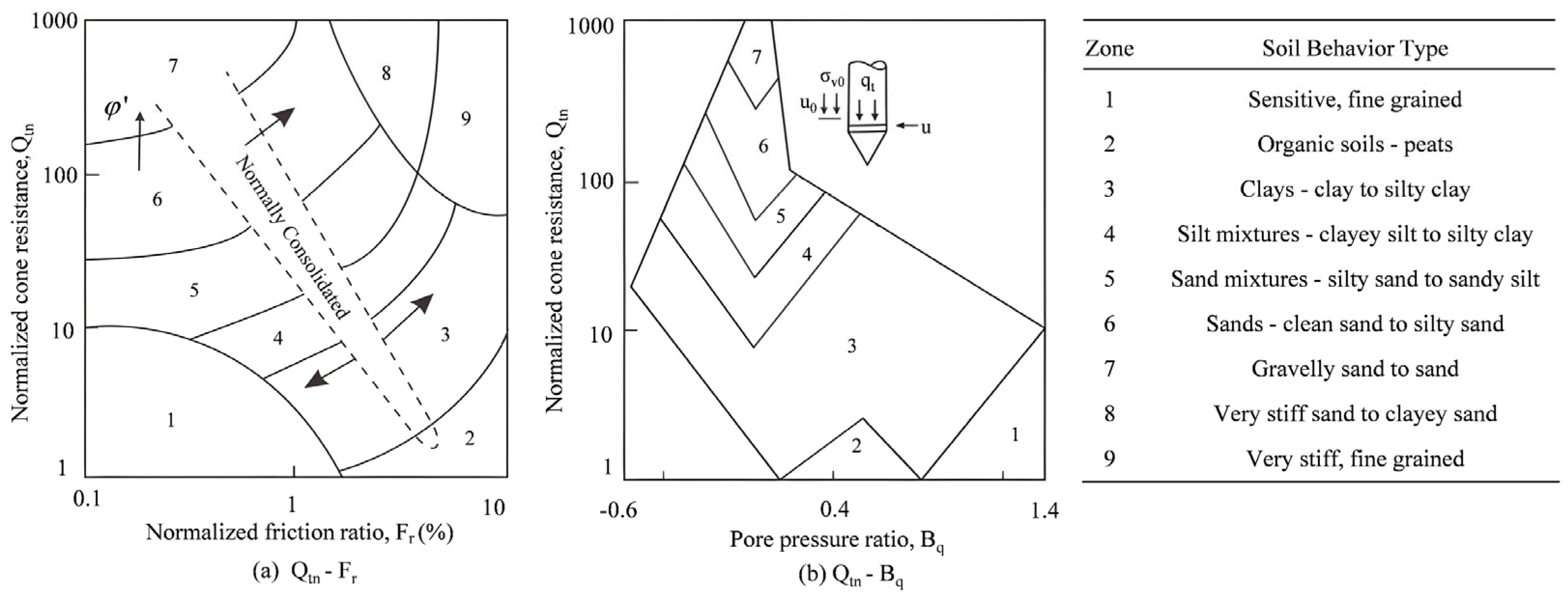
In 2009, Robertson updated his earlier soil behavior type charts, as illustrated in Figure 3a,b, by introducing the stress-normalized cone resistance (Q_tn), in which an exponent n was incorporated to account for stress level effects. The formulas for Q_tn and n are shown in Equation (6) and Equation (7), respectively.

$$Q_{tn}=\left({\displaystyle \frac{q_t-{\sigma }_{v0}}{p_a}}\right){\left({\displaystyle \frac{p_a}{{{\sigma }^{\prime }}_{v0}}}\right)}^n$$

(6)

$$n=0.381I_c+0.05\left({\displaystyle \frac{\sigma {\prime }_{v0}}{p_a}}\right)-0.15$$

(7)

where p_a is the atmospheric pressure.

The numbered zones in these charts correspond to distinct soil behavior types. For the purpose of constructing supervised-learning labels, each soil behavior type was mapped to a model output class: Sensitive, fine-grained → Class 1; Organic soils—peats → Class 2; Clays—clay to silty clay → Class 3; Silt mixtures—clayey silt to silty clay → Class 4; Sand mixtures—silty sand to sandy silt → Class 5; Sands—clean sand to silty sand → Class 6; Gravelly sand to sand → Class 7; Very stiff sand to clayey sand → Class 8; and Very stiff, fine grained → Class 9.

2.2.2. Dataset Partitioning

The dataset was partitioned according to two key principles: clarity of purpose and spatial independence. Clarity of purpose means that, according to the research objectives, data from different regions were explicitly partitioned into training and test sets. The training set was employed for model training and validation, whereas the test sets were reserved for independent evaluation of generalization performance. Spatial independence required that the training and test sets be completely separated geographically, with no overlapping areas, ensuring that the test sets can accurately reflect the model’s performance in previously unseen regions.

Three representative regions were selected from the dataset as independent test sets, while data from all other regions were combined to form the training set. The sample counts for the training and test sets are summarized in

Table 2. Sample distribution of training and independent test sets with Classes 1–9.

Dataset	Country	Class 1	Class 2	Class 3	Class 4	Class 5	Class 6	Class 7	Class 8	Class 9	Total
Train set	Austria	1769	5246	51,763	23,679	42,646	31,396	3868	1545	2061	163,973
	New Zealand	512	688	22,899	27,969	40,688	58,919	9383	2839	7310	171,207
	The Netherlands	29	18,732	9470	3184	2318	34	0	0	6	33,773
	USA	0	21	2190	2022	528	89	40	134	1364	6388
	Italy	1	1648	30,074	3704	1561	1222	23	23	588	38,844
	Japan	30	25	519	187	231	702	8	41	37	1780
	China	1074	10	3148	4989	16,952	11,989	44	13	0	38,219
Test set	New Zealand (Richmond)	15	32	1150	1311	1722	1035	17	1350	3881	10,513
	New Zealand (Port Nelson)	226	502	1940	1694	1896	3982	194	143	82	10,659
	USA (Hollywood)	24	80	1545	2055	4064	8049	280	205	123	16,425

. The training set contains 454,184 samples, while the three independent test sets are from Richmond and Port Nelson in New Zealand, and Hollywood in the United States. Each test site is geographically separated from the training set by more than 100 km, ensuring spatial independence. They also exhibit distinct differences in class composition. The Richmond test set contains the minority classes (Class 8 and Class 9) from the training set, while the Port Nelson test set contains the minority classes (Class 1 and Class 2). The class distribution of the Hollywood test set is similar to that of the training set, mainly consisting of Classes 3–6. Overall, the three test sets differ in their class distributions, offering diverse conditions to assess the model’s cross-regional generalization performance.

2.2.3. Data Standardization

Data standardization is a process that transforms data through specific mathematical operations, mapping them onto a unified range or distribution. Since the input features differ significantly in magnitude, directly feeding them into the model may cause features with larger values to dominate the results. To avoid such bias and ensure that different features are compared on the same scale, this study applies Z-score standardization for data preprocessing. For each feature x, we compute:

$$x*={\displaystyle \frac{x-\mu }{\sigma }}$$

(8)

where μ and σ are the feature mean and standard deviation computed from the training set, and x* denotes the standardized value of the feature.

2.3. Machine Learning Model

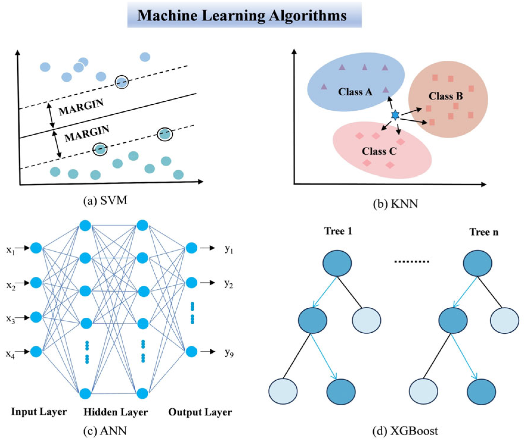
Machine learning (ML) has become an essential tool for analyzing large-scale geotechnical data. By learning nonlinear mappings from input features to target labels, ML can capture complex patterns from large volumes of training data. In this study, we evaluated four supervised algorithms: Support Vector Machine (SVM), K-Nearest Neighbors (KNN), Artificial Neural Network (ANN), and Extreme Gradient Boosting (XGBoost).

The Support Vector Machine (SVM) operates by identifying a separating hyperplane with the maximum margin in the feature space, which improves classification robustness. Figure 4a illustrates a linear SVM. Earlier studies have reported that SVM can be effective in handling minority soil classes [36].

The K-Nearest Neighbors (KNN) is an intuitive and commonly employed supervised learning algorithm. As illustrated in Figure 4b, it classifies a test sample by computing its distances to the training samples, selecting the k nearest ones, and inferring the label based on their classes. In classification tasks, the class occurring most frequently among the neighbors is usually assigned as the prediction [32].

The Artificial Neural Network (ANN) is a computational model inspired by biological neural systems. As shown in Figure 4c, it comprises an input layer, one or more hidden layers, and an output layer, with neurons in each layer linked through weighted connections to enable information transfer and processing. Training typically involves initialization, forward propagation, loss calculation, backpropagation, and parameter updating, repeated until convergence or predefined stopping criteria are satisfied [34].

The Extreme Gradient Boosting (XGBoost) uses decision trees as base weak learners and iteratively builds multiple weak models within the gradient boosting framework, combining them through weighted aggregation to form a more powerful ensemble model, as illustrated in Figure 4d. In each iteration, XGBoost generates a new tree by minimizing an objective function composed of a loss function and a regularization term, fitting the current residuals, and progressively optimizing the overall model performance [49].

To examine the impact of different feature combinations on classification performance and model generalization, three sets of input features were compared in this study: (1) Depth, q_c, f_s, u₂: original measured parameters to assess the model’s ability to learn from raw measurements; (2) Depth, q_t, R_f, B_q: incorporating derived parameters to examine their contribution to classification accuracy; (3) Depth, q_t, R_f, B_q, F_r, u₂: the second set was expanded with F_r and u₂ to assess whether these additional features improve classification performance.

2.4. Performance Evaluation Metrics

In classification performance evaluation, the core is the confusion matrix calculated on the test set, from which various performance metrics are derived.

Table 3. Definition of True Positive, False Negative, False Positive, and True Negative in the confusion matrix.

		Predicted
		Positive	Negative
Actual	Positive	True Positive (TP)	False Negative (FN)
	Negative	False Positive (FP)	True Negative (TN)

illustrates the structure of the confusion matrix, where True Positive (TP): number of samples that are truly positive and predicted as positive; False Negative (FN): number of samples that are truly positive but incorrectly predicted as negative; False Positive (FP): number of samples that are truly negative but incorrectly predicted as positive; True Negative (TN): number of samples that are truly negative and predicted as negative.

This study also employs commonly used metrics in classification tasks—Balanced accuracy, F₁-weighted, and Cohen’s Kappa (Kappa)—to evaluate model performance from multiple perspectives. Due to the significant class imbalance in the test set, using accuracy may obscure the model’s ability to correctly identify minority soil classes. Balanced accuracy, which averages the recall of each class, provides a more equitable assessment of the model’s performance across different classes:

$$\begin{array}{c}\mathit{Balanced} \mathit{accuracy}\end{array}={\displaystyle \frac{1}{K}}{\displaystyle \sum _{i=1}^K\frac{T{P}_i}{T{P}_i+F{N}_i}}$$

(9)

where K is the number of classes, TP_i and FN_i are the number of true positives and false negatives for class i, respectively.

F₁-weighted combines precision and recall, weighting each class according to its sample size, thereby reflecting the overall predictive quality of the model under the true data distribution:

$$\begin{array}{c}{F}_1-\mathit{weighted}\end{array}={\displaystyle \sum _{i=1}^K\frac{N_i}{N}}\cdot {\displaystyle \frac{2\cdot T{P}_i}{2\cdot T{P}_i+F{P}_i+F{N}_i}}$$

(10)

where N_i is the number of samples in class i, and N is the total number of samples. FP_i is the number of false positives for class i.

Cohen’s Kappa (Kappa) accounts for agreement occurring by chance, providing a more stringent and reliable measure of model performance than simple accuracy:

$$\mathit{kappa}={\displaystyle \frac{P_{\mathrm{o}}-P_e}{1-P_e}}$$

(11)

where P_o and P_e represent the observed accuracy and the expected accuracy, respectively.

3. Results

3.1. Performance Evaluation on the Test Set

This study compares the performance of four machine learning algorithms (SVM, KNN, ANN, and XGBoost) across three feature combinations for soil classification. Models are trained using 5-fold cross-validation, and their hyperparameters are optimized via Bayesian optimization. Each model is evaluated on three independent test sets (Richmond, Port Nelson, and Hollywood), reporting Balanced accuracy, F₁-weighted, and Kappa, and presenting confusion matrices to analyze the distribution of classification errors.

3.1.1. Performance Evaluation on the Richmond Test Set

The performance evaluation on the Richmond test set is summarized in

Table 4. Performance evaluation of SVM, KNN, ANN, and XGBoost on the Richmond test set across three feature combinations.

Feature Combinations	Algorithms	Balanced Accuracy	F1-Weighted	Kappa
Depth, qc, fs, u2	SVM	0.531	0.625	0.576
	KNN	0.632	0.657	0.642
	ANN	0.641	0.667	0.652
	XGBoost	0.814	0.944	0.923
Depth, qt, Rf, Bq	SVM	0.628	0.689	0.653
	KNN	0.735	0.766	0.758
	ANN	0.752	0.782	0.763
	XGBoost	0.846	0.948	0.928
Depth, qt, Rf, Bq, Fr, u2	SVM	0.762	0.792	0.774
	KNN	0.832	0.851	0.848
	ANN	0.829	0.871	0.843
	XGBoost	0.929	0.966	0.956

. Under a fixed feature combination, comparison of different algorithms shows that XGBoost outperforms SVM, KNN, and ANN on all evaluation metrics. When holding the algorithm constant and comparing different feature combinations, the feature set comprising raw measurements performs relatively poorly; performance improves markedly after the introduction of derived parameters, and improves further when F_r and u₂ are added. In particular, the XGBoost algorithm with the feature set Depth, q_t, R_f, B_q, F_r, u₂ achieves Balanced accuracy 0.929, F₁-weighted 0.966, and Kappa 0.956—the best performance among the twelve evaluated models. The corresponding confusion matrix for this model is given in

Table 5. Confusion matrix of the XGBoost algorithm with feature set Depth, q_t, R_f, B_q, F_r, u₂ on the Richmond test set.

Richmond		Confusion Matrix
		Predicted
		1	2	3	4	5	6	7	8	9
Actual	1	13	0	0	0	1	1	0	0	0
	2	0	25	7	0	0	0	0	0	0
	3	0	0	1127	13	0	0	0	0	10
	4	0	0	16	1256	11	0	0	0	28
	5	0	0	0	19	1656	27	0	20	0
	6	3	0	0	0	27	1004	0	1	0
	7	1	0	0	0	0	0	16	0	0
	8	0	0	0	4	38	25	0	1246	37
	9	0	0	25	30	0	0	0	16	3810

Note: The numerical labels on the rows and columns in the table correspond to the following soil behavior types. 1—Sensitive, fine-grained; 2—Organic soils—peats; 3—Clays—clay to silty clay; 4—Silt mixtures—clayey silt to silty clay; 5—Sand mixtures—silty sand to sandy silt; 6—Sands—clean sand to silty sand; 7—Gravelly sand to sand; 8—Very stiff sand to clayey sand; 9—Very stiff, fine grained. (The same labeling convention applies to Table 7 and Table 9).

. The confusion matrix provides an intuitive view of the distribution of correct and incorrect predictions on the test set: diagonal entries represent the numbers of correctly predicted samples (bolded), where larger diagonal values indicate higher classification accuracy; off-diagonal entries correspond to misclassifications. Specifically, Class 3, Class 4, Class 5, Class 8, and Class 9 show strong predictive performance, as their diagonal counts substantially exceed misclassification counts. Misclassifications are mainly concentrated between adjacent classes (Class 3 ↔ Class 4, Class 4 ↔ Class 5, and Class 5 ↔ Class 6), which is likely due to the continuous transitions in soil characteristics and CPTU signals, as well as the inherent fuzziness of class boundaries.

3.1.2. Performance Evaluation on the Port Nelson Test Set

The performance evaluation on the Port Nelson test set is summarized in

Table 6. Performance evaluation of SVM, KNN, ANN, and XGBoost on the Port Nelson test set across three feature combinations.

Feature Combinations	Algorithms	Balanced Accuracy	F1-Weighted	Kappa
Depth, qc, fs, u2	SVM	0.573	0.618	0.603
	KNN	0.665	0.692	0.675
	ANN	0.702	0.783	0.751
	XGBoost	0.827	0.883	0.848
Depth, qt, Rf, Bq	SVM	0.632	0.674	0.658
	KNN	0.725	0.753	0.748
	ANN	0.718	0.743	0.724
	XGBoost	0.923	0.961	0.947
Depth, qt, Rf, Bq, Fr, u2	SVM	0.743	0.782	0.765
	KNN	0.835	0.882	0.867
	ANN	0.848	0.872	0.865
	XGBoost	0.937	0.969	0.959

. The same conclusion as for the Richmond test set holds: the XGBoost algorithm with the feature set Depth, q_t, R_f, B_q, F_r, u₂ achieves Balanced accuracy 0.937, F₁-weighted 0.969, and Kappa 0.959. The corresponding confusion matrix is presented in

Table 7. Confusion matrix of the XGBoost algorithm with feature set Depth, q_t, R_f, B_q, F_r, u₂ on the Port Nelson test set.

Port Nelson		Confusion Matrix
		Predicted
		1	2	3	4	5	6	7	8	9
Actual	1	198	0	0	6	22	0	0	0	0
	2	0	497	5	0	0	0	0	0	0
	3	0	12	1888	39	0	0	0	0	1
	4	33	0	36	1563	62	0	0	0	0
	5	7	0	0	14	1861	13	0	1	0
	6	2	0	0	0	24	3940	8	8	0
	7	0	0	0	0	0	20	174	0	0
	8	0	0	0	2	4	3	0	134	0
	9	0	0	8	2	0	0	0	1	71

. Port Nelson contains more samples of Class 1 and Class 2 than Richmond; the model remains robust across different class distributions. Misclassifications remain concentrated among adjacent classes—especially between Class 3, Class 4, and Class 5—while other classes show misclassification to varying degrees but at lower frequency.

3.1.3. Performance Evaluation on the Hollywood Test Set

On the Hollywood test set, the performance of most models improves, as shown in

Table 8. Performance evaluation of SVM, KNN, ANN, and XGBoost on the Hollywood test set across three feature combinations.

Feature Combinations	Algorithms	Balanced Accuracy	F1-Weighted	Kappa
Depth, qc, fs, u2	SVM	0.728	0.752	0.736
	KNN	0.783	0.831	0.792
	ANN	0.803	0.825	0.816
	XGBoost	0.868	0.953	0.930
Depth, qt, Rf, Bq	SVM	0.776	0.793	0.782
	KNN	0.891	0.923	0.905
	ANN	0.918	0.952	0.947
	XGBoost	0.967	0.980	0.969
Depth, qt, Rf, Bq, Fr, u2	SVM	0.863	0.906	0.885
	KNN	0.901	0.942	0.927
	ANN	0.914	0.961	0.938
	XGBoost	0.972	0.982	0.973

. This may be attributed to the higher geological similarity between this test set and the training set, which reduces domain shift and enhances classification accuracy. When the input feature combination is Depth, q_t, R_f, B_q, F_r, u₂, XGBoost again delivers the best performance, with Balanced accuracy 0.972, F₁-weighted 0.982, and Kappa 0.973. The corresponding confusion matrix is presented in

Table 9. Confusion matrix of the XGBoost algorithm with feature set Depth, q_t, R_f, B_q, F_r, u₂ on the Hollywood test set.

Hollywood		Confusion Matrix
		Predicted
		1	2	3	4	5	6	7	8	9
Actual	1	23	0	0	1	0	0	0	0	0
	2	0	78	2	0	0	0	0	0	0
	3	0	0	1522	23	0	0	0	0	0
	4	3	0	17	2008	27	0	0	0	0
	5	9	0	0	41	3956	57	0	1	0
	6	0	0	0	0	61	7963	20	5	0
	7	0	0	0	0	0	16	264	0	0
	8	0	0	0	0	5	3	0	195	2
	9	0	0	1	0	0	0	0	0	122

. Both majority classes (Class 3, Class 4, Class 5, Class 6) and minority classes (Class 1, Class 2, Class 7, Class 8, Class 9) maintain high recognition rates, with misclassifications still concentrated along adjacent class boundaries.

3.2. Stratigraphic Prediction on Unseen CPTU Data

Based on the feature combination of Depth, q_t, R_f, B_q, F_r, and u₂, the XGBoost algorithm achieved the best performance across three independent test sets. Therefore, this model was applied to the unseen CPTU data from the Guangzhou site (China) and the New Lock site (The Netherlands) to perform stratigraphic prediction.

3.2.1. CPTU Data from Guangzhou

Figure 5 shows, from left to right, the CPTU measurements (q_c and f_s) at the Guangzhou site, the stratigraphy predicted by the model, Robertson’s SBTn-based classification, and the stratigraphy from an adjacent borehole. According to borehole data, the stratigraphy is dominated by Class 3, Class 5, and Class 6. The model reproduces these main units with high consistency and additionally resolves finer details: in the shallow layer (3–18 m), Classes 3–6 are alternately distributed; in the middle layer (18–39 m), Classes 3–5 are present; in the deep layer (39–61 m), the model identifies interbedded Class 4. Comparison with Robertson’s SBTn-based classification reveals a strong overall agreement, particularly in the shallow and middle sections where soil types alternate, indicating the model’s ability to accurately delineate complex stratigraphic distributions.

3.2.2. CPTU Data from New Lock

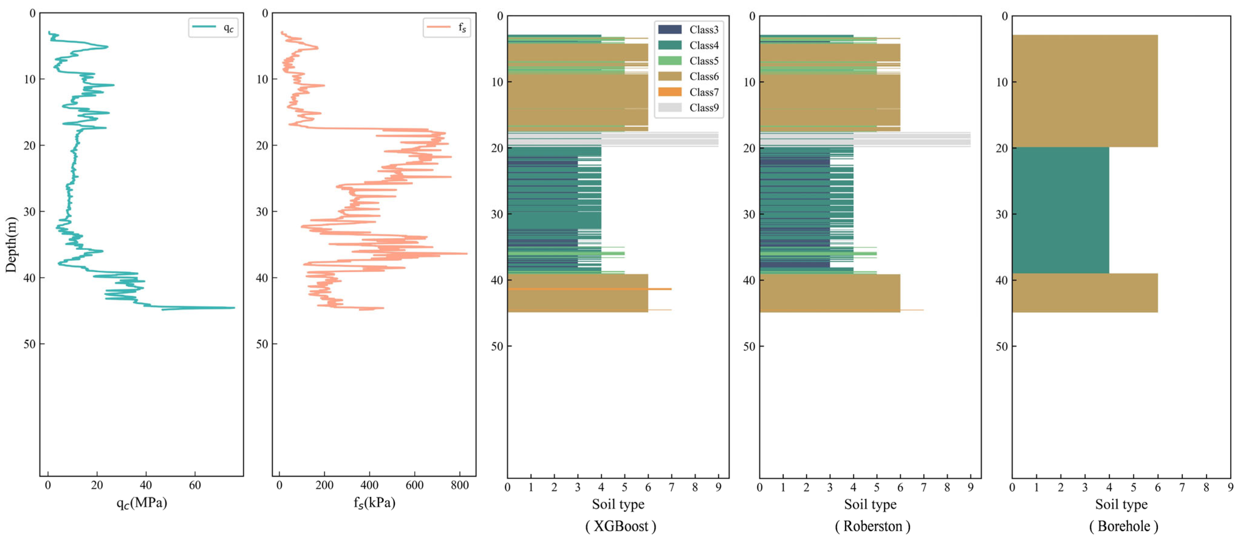
This model was also applied to the New Lock site in the Netherlands, and the predicted results are presented in Figure 6. Overall, the model’s prediction is consistent with the main layers revealed by borehole data. In the shallow layer (3–18 m), both q_c and f_s remain relatively stable, and the model identifies Classes 4–6; at 18–20 m, a sudden increase in f_s occurs, and the model successfully identifies Class 9; in the middle layer (20–39 m), the model detects an alternating distribution of Classes 3–5, while in the deep layer (39–45 m), Class 6 dominates with minor occurrences of Class 7. The model prediction is highly consistent with Robertson’s SBTn-based classification, further indicating that the model effectively captures the nonlinear relationships among CPTU data corresponding to different soil types and demonstrates potential for practical engineering applications.

3.3. Feature Importance Analysis

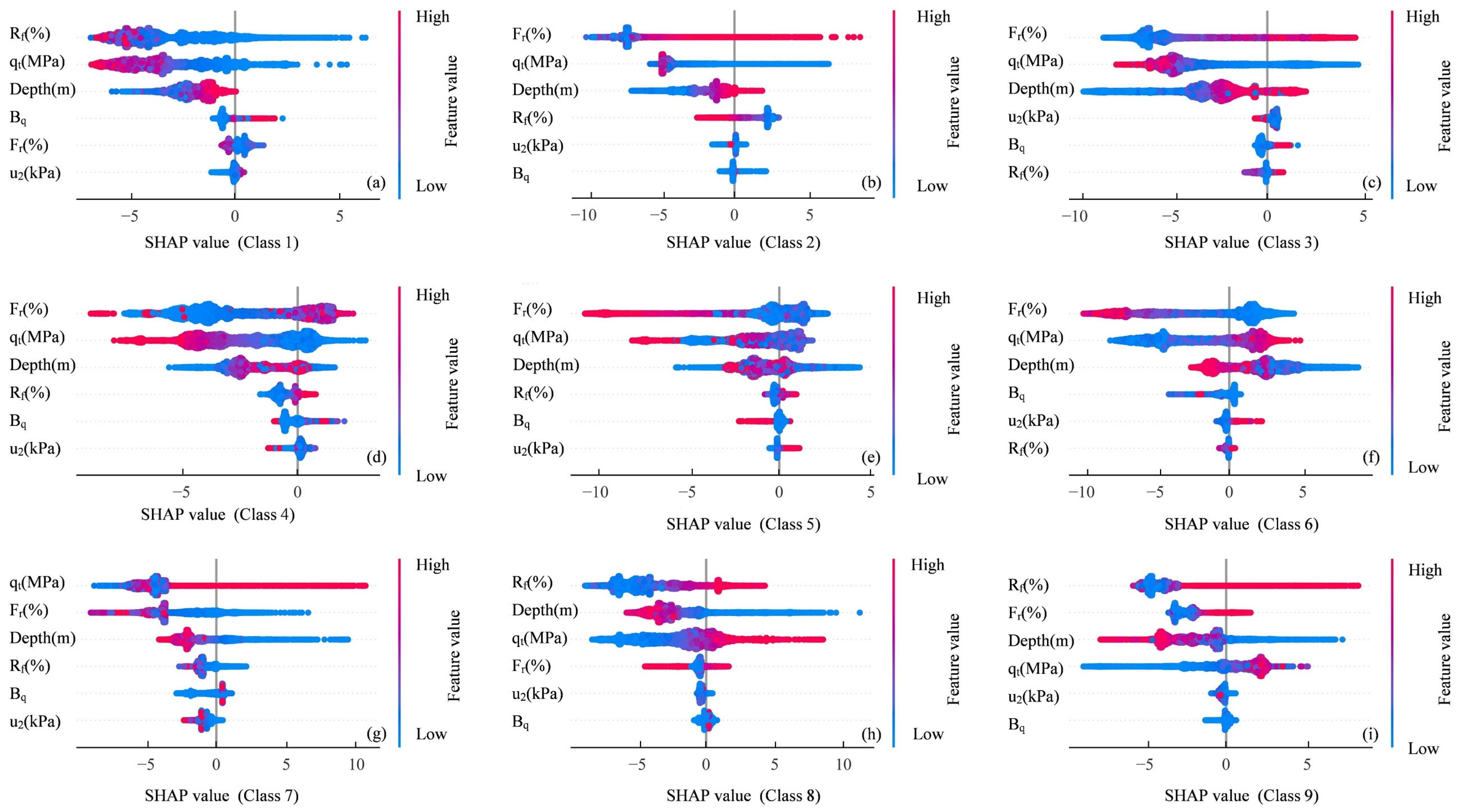
In this section, SHAP (SHapley Additive exPlanations) is applied to interpret the XGBoost algorithm trained with the feature set Depth, q_t, R_f, B_q, F_r, and u₂. This analysis provides insights into the contribution of each feature to class predictions. Figure 7 presents the feature-level explanations across the nine classes. Each point denotes the SHAP value of a specific observation for a given feature, with the x-axis representing the SHAP value and the color gradient reflecting the magnitude of the feature value from low (blue) to high (red). Features are ranked by importance, where larger absolute SHAP values indicate a more significant influence on the predictions [49].

The SHAP analysis indicates that F_r and q_t are the two most influential predictors, as measured by mean absolute SHAP values across classes. Specifically, F_r exhibits positive SHAP values for Class 3, implying that higher F_r increases the model’s predicted score—whereas it contributes negatively to Classes 5–7, implying that higher F_r reduces the model’s predicted score (and thus the predicted probability) for those classes. High q_t is positively associated with predictions of Classes 6–8 and tends to reduce predicted scores for Classes 3–4. R_f shows effects in several minority classes: high R_f increases predicted scores for Classes 8–9 but tends to decrease the predicted score for Class 1. Depth displays a more balanced distribution of SHAP values across classes. In contrast, B_q and u₂ have low mean absolute SHAP values and exhibit no consistent directional trend across most classes.

These SHAP-derived relationships are consistent with known geotechnical mechanisms underlying soil behavior. A higher F_r, generally reflects finer-grained, more cohesive, and less permeable soils. The positive SHAP contribution of F_r to Class 3 and its negative influence on sand-dominated Classes 5–7 therefore align with the mechanical behavior of cohesive soils, where high frictional resistance arises from greater adhesion and lower drainage capacity. Conversely, high q_t indicates dense or well-consolidated sands with higher strength and stiffness, which explains its strong positive SHAP association with Classes 6–8 and its negative association with softer fine-grained Classes 3–4. The observed effects of R_f and Depth also follow typical geotechnical trends: deeper strata and higher R_f values are often linked to over consolidated or cemented layers, corresponding to Classes 8–9 characterized by high strength and stiffness.

4. Discussion

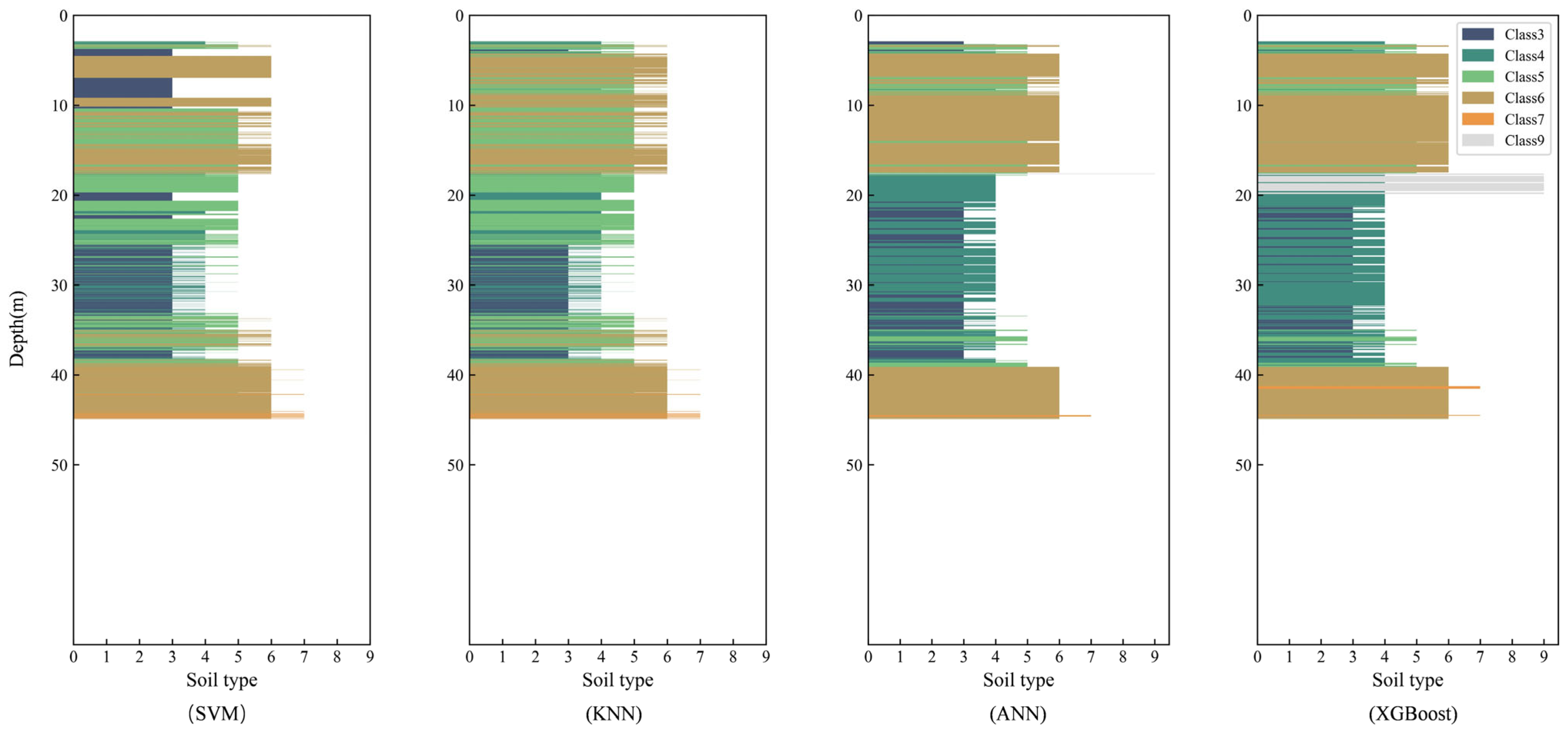
Results in Section 3.1 indicate that XGBoost achieved the best performance across the three test sets. In Section 3.2, the model was further applied to unseen data from Guangzhou and New Lock, where it also exhibited strong predictive capability. To investigate why SVM, KNN, and ANN underperformed relative to XGBoost, we applied these three algorithms to the same unseen data from Guangzhou and New Lock used in Section 3.2. Figure 8 and Figure 9, respectively, illustrate the stratigraphic predictions of the four algorithms for the two sites.

First, in the strata of both Guangzhou and New Lock, the primary misclassifications by SVM, KNN, and ANN occurred between adjacent soil classes with similar physical and behavioral characteristics (Class 3 ↔ Class 4, Class 4 ↔ Class 5, Class 5 ↔ Class 6), with error rates markedly higher than those of XGBoost. Second, these models exhibited limited capability in detecting interbeds—for example, the Class 9 interbed at 18–20 m in the New Lock strata was not correctly identified by any of the three algorithms. Finally, stratigraphically complex zones emerged as the major sources of misclassification. In particular, the intervals of 39–64 m in Guangzhou and 20–39 m in New Lock contain frequent alternations of soil types. Within these transitional layers, the misclassifications of these three algorithms were highly concentrated, often forming continuous or block-like error segments. This indicates that these algorithms lack sufficient robustness in handling local complexity and class boundaries.

From an algorithmic perspective, SVM can be sensitive to high-dimensional input features and class imbalance, which may lead to systematic misclassification. KNN is strongly influenced by the distribution of training samples as well as by the distance metric. When some classes occur more frequently than others, it tends to assign test instances to the majority class, resulting in higher omission rates for minority classes. ANN, due to its large number of parameters, is prone to overfitting during training and shows high sensitivity to initial weights and network design. In contrast, XGBoost, as a tree-based ensemble approach, has clear advantages in dealing with nonlinear relationships and class imbalance. By means of stepwise splitting and regularization, it can better capture complex decision boundaries, which explains its stronger performance in stratigraphically complex alternating layers. This indicates that XGBoost provides more stable and reliable results in cross-regional soil classification tasks with frequent stratigraphic changes.

This study developed a soil classification model based on cross-regional CPTU data, which demonstrated strong performance in typical geological settings such as valleys, basins, glaciers, and deltas. However, the training data are concentrated in limited regions and specific geological environments, with insufficient coverage of complex or challenging geological conditions such as karst terrains, red clay, tropical weathering crusts, and weakly structured soils. When the model is applied to regions with geological environments similar to those in the training samples (such as basins), it can identify soil types and stratigraphic distributions. While the model is applied to geologically distinct environments (such as karst), its generalization performance may decrease due to the lack of similar training samples, leading to increased uncertainty in the predictions. In addition, CPTU parameters vary continuously, and the boundaries between soil types are not sharply defined, often overlapping across classes. For example, in transitional strata such as silty clay and silt, the absence of clear boundaries introduces uncertainty into the model’s predictions, thereby reducing the consistency and accuracy of stratigraphic interpretation. Another limitation is that, predictive uncertainty in CPTU-based classification arises from multiple sources: measurement noise in q_c, f_s and u₂; label uncertainty introduced when mapping CPTU signals to discrete SBTn classes; class imbalance and limited samples for minority classes.

To address these limitations, future work may follow three directions. First, expanding the cross-regional dataset to include a more diverse set of geological settings will improve the model’s generalizability across a wider range of engineering scenarios. Moreover, testing the model on entirely unfamiliar geological regions—such as areas with distinctly different lithology, stratigraphic sequences, or tectonic settings—would provide a more rigorous evaluation of its extreme generalization capability. Second, differences in CPTU equipment, cone geometry, and testing procedures may introduce systematic biases. Therefore, future work will involve dedicated inter-instrument calibration efforts, including the collection of instrument metadata, paired-site testing, and the development of correction or domain-adaptation models, to further enhance the model’s cross-regional robustness. Third, employing stronger 1D sequence models—such as Transformer-based encoders or TCN–Transformer hybrids—can more effectively capture long-range dependencies along the depth dimension [50].

5. Conclusions

(1)

The dataset for this study integrates the Premstaller Geotechnik database, the Global-CPT/3/1196 database, and a Chinese engineering project database. It encompasses samples from multiple countries and diverse geological environments (basins, valleys, glaciers, and deltas).

(2)

The model using the feature set Depth, q_t, R_f, B_q, F_r, u_2, and the XGBoost algorithm performed best. Compared with SVM, KNN, and ANN, XGBoost can better capture nonlinear relationships and handle class imbalance in soil classification, while its regularization effectively reduces the risk of overfitting, leading to better predictive reliability.

(3)

The model demonstrates strong predictive capability when applied to new sites, showing well adaptability to unseen data. In engineering practice, it can be used as a rapid and cost-effective tool for preliminary stratigraphic interpretation and soil-type identification in tunneling, foundation, and slope projects, supplementing conventional borehole investigations.

References

1. Begemann, H.K.S. The Friction Jacket Cone as an Aid in Determining the Soil Profile. In Proceedings of the Sixth International Conference on Soil Mechanics and Foundation Engineering, Montreal, QC, Canada, 8–15 September 1965; ISSMGE: Montreal, QC, Canada, 1965; pp. 17–20. [Google Scholar]
2. Schmertmann, J.H. Guidelines for Cone Penetration Test: Performance and Design; U.S. Department of Transportation: Washington, DC, USA, 1978. [Google Scholar]
3. Douglas, B.J.; Olsen, R.S. Soil Classification Using Electric Cone Penetrometer. In Proceedings of the Conference on Cone Penetration Testing and Experience, St. Louis, MO, USA, 26–30 October 1981; ASCE: St. Louis, MO, USA, 1981; pp. 209–227. [Google Scholar]
4. Robertson, P.K.; Campanella, R.G. Interpretation of Cone Penetration Tests. Part I: Sand. Can. Geotech. J. 1983, 20, 718–733. [Google Scholar] [CrossRef]
5. Robertson, P.K. Soil Classification Using the Cone Penetration Test. Can. Geotech. J. 1990, 27, 151–158. [Google Scholar] [CrossRef]
6. Jefferies, M.; Davies, M. Use of CPTu to Estimate Equivalent SPT N60. Geotech. Test. J. 1993, 16, 458–468. [Google Scholar] [CrossRef]
7. Schneider, J.A.; Randolph, M.F.; Mayne, P.W.; Ramsey, N.R. Analysis of Factors Influencing Soil Classification Using Normalized Piezocone Tip Resistance and Pore Pressure Parameters. J. Geotech. Geoenviron. Eng. 2008, 134, 1569–1586. [Google Scholar] [CrossRef]
8. Robertson, P.K. Cone Penetration Test (CPT)-Based Soil Behaviour Type (SBT) Classification System—An Update. Can. Geotech. J. 2016, 53, 1910–1927. [Google Scholar] [CrossRef]
9. Eslami, A.; Heidarie Golafzani, S.; Naghibi, M.H. Developed Triangular Charts; Deltaic CPTu-Based Soil Behavior Classification Using AUT: CPTu-Geo-Marine Database. Probabilistic Eng. Mech. 2023, 71, 103380. [Google Scholar] [CrossRef]
10. Hegazy, Y.A.; Mayne, P.W. Objective Site Characterization Using Clustering of Piezocone Data. J. Geotech. Geoenviron. Eng. 2002, 128, 986–996. [Google Scholar] [CrossRef]
11. Facciorusso, J.; Uzielli, M. Stratigraphic Profiling by Cluster Analysis and Fuzzy Soil Classification from Mechanical Cone Penetration Tests. In Proceedings of the 2nd International Conference on Site Characterization ISC-2, Porto, Portugal, 19–22 September 2004; Millpress: Rotterdam, The Netherlands, 2004; pp. 905–912. [Google Scholar]
12. Liao, T.; Mayne, P.W. Stratigraphic Delineation by Three-Dimensional Clustering of Piezocone Data. Georisk Assess. Manag. Risk Eng. Syst. Geohazards 2007, 1, 102–119. [Google Scholar] [CrossRef]
13. Das, S.K.; Basudhar, P.K. Utilization of Self-Organizing Map and Fuzzy Clustering for Site Characterization Using Piezocone Data. Comput. Geotech. 2009, 36, 241–248. [Google Scholar] [CrossRef]
14. Wang, X.; Wang, H.; Liang, R.Y.; Liu, Y. A Semi-Supervised Clustering-Based Approach for Stratification Identification Using Borehole and Cone Penetration Test Data. Eng. Geol. 2019, 248, 102–116. [Google Scholar] [CrossRef]
15. Carvalho, L.O.; Ribeiro, D.B. Application of Kernel K-Means and Kernel x-Means Clustering to Obtain Soil Classes from Cone Penetration Test Data. Soils Rocks 2020, 43, 607–618. [Google Scholar] [CrossRef]
16. Hudson, K.S.; Ulmer, K.J.; Zimmaro, P.; Kramer, S.L.; Stewart, J.P.; Brandenberg, S.J. Unsupervised Machine Learning for Detecting Soil Layer Boundaries from Cone Penetration Test Data. Earthq. Eng. Struct. Dyn. 2023, 52, 3201–3215. [Google Scholar] [CrossRef]
17. Jung, B.-C.; Gardoni, P.; Biscontin, A. Probabilistic Soil Identification Based on Cone Penetration Tests. Géotechnique 2008, 58, 591–603. [Google Scholar] [CrossRef]
18. Cetin, K.O.; Ozan, C. CPT-Based Probabilistic Soil Characterization and Classification. J. Geotech. Geoenviron. Eng. 2009, 135, 84–107. [Google Scholar] [CrossRef]
19. Wang, Y.; Huang, K.; Cao, Z. Probabilistic Identification of Underground Soil Stratification Using Cone Penetration Tests. Can. Geotech. J. 2013, 50, 766–776. [Google Scholar] [CrossRef]
20. Depina, I.; Le, T.M.H.; Eiksund, G.; Strøm, P. Cone Penetration Data Classification with Bayesian Mixture Analysis. Georisk Assess. Manag. Risk Eng. Syst. Geohazards 2016, 10, 27–41. [Google Scholar] [CrossRef]
21. Cao, Z.-J.; Zheng, S.; Li, D.-Q.; Phoon, K.-K. Bayesian Identification of Soil Stratigraphy Based on Soil Behaviour Type Index. Can. Geotech. J. 2019, 56, 570–586. [Google Scholar] [CrossRef]
22. Hu, Y.; Wang, Y. Probabilistic Soil Classification and Stratification in a Vertical Cross-Section from Limited Cone Penetration Tests Using Random Field and Monte Carlo Simulation. Comput. Geotech. 2020, 124, 103634. [Google Scholar] [CrossRef]
23. Várady, C.; Tenório, J.; Silva, E.; Lima Junior, E.; Santos, J.; Dias, R.; Cutrim, F. Bayesian-Based Approach in Soil Characterization for Tophole Design. SPE J. 2024, 29, 5792–5803. [Google Scholar] [CrossRef]
24. Han, X.; Gong, W.; Juang, C.H. Probabilistic Evaluation of Earthquake-Induced Liquefaction Using Bayesian Network Based on a Side-by-Side SPT–CPT Database. Can. Geotech. J. 2024, 61, 2653–2666. [Google Scholar] [CrossRef]
25. Kurup, P.U.; Griffin, E.P. Prediction of Soil Composition from CPT Data Using General Regression Neural Network. J. Comput. Civ. Eng. 2006, 20, 281–289. [Google Scholar] [CrossRef]
26. Arel, E. Predicting the Spatial Distribution of Soil Profile in Adapazari/Turkey by Artificial Neural Networks Using CPT Data. Comput. Geosci. 2012, 43, 90–100. [Google Scholar] [CrossRef]
27. Cai, G.; Liu, S.; Puppala, A.J.; Tong, L. Identification of Soil Strata Based on General Regression Neural Network Model from CPTU Data. Mar. Georesources Geotechnol. 2015, 33, 229–238. [Google Scholar] [CrossRef]
28. Miao, Y.; Bai, G. Soil Layer Interface Identification Using Piezocone Penetration Test Based on Probabilistic Neural Network. J. Univ. Jinan Sci. Technol. 2017, 31, 279–284. [Google Scholar]
29. Reale, C.; Gavin, K.; Librić, L.; Jurić-Kaćunić, D. Automatic Classification of Fine-Grained Soils Using CPT Measurements and Artificial Neural Networks. Adv. Eng. Inform. 2018, 36, 207–215. [Google Scholar] [CrossRef]
30. Ghaderi, A.; Abbaszadeh Shahri, A.; Larsson, S. An Artificial Neural Network Based Model to Predict Spatial Soil Type Distribution Using Piezocone Penetration Test Data (CPTu). Bull. Eng. Geol. Environ. 2019, 78, 4579–4588. [Google Scholar] [CrossRef]
31. Erharter, G.H.; Oberhollenzer, S.; Fankhauser, A.; Marte, R.; Marcher, T. Learning Decision Boundaries for Cone Penetration Test Classification. Comput.-Aided Civ. Infrastruct. Eng. 2021, 36, 489–503. [Google Scholar] [CrossRef]
32. Carvalho, L.O.; Ribeiro, D.B. Soil Classification System from Cone Penetration Test Data Applying Distance-Based Machine Learning Algorithms. Soils Rocks 2019, 42, 167–178. [Google Scholar] [CrossRef]
33. Godoy, C.; Depina, I.; Thakur, V. Application of Machine Learning to the Identification of Quick and Highly Sensitive Clays from Cone Penetration Tests. J. Zhejiang Univ.-Sci. A 2020, 21, 445–461. [Google Scholar] [CrossRef]
34. Rauter, S.; Tschuchnigg, F. CPT Data Interpretation Employing Different Machine Learning Techniques. Geosciences 2021, 11, 265. [Google Scholar] [CrossRef]
35. Carvalho, L.O.; Ribeiro, D.B. A Multiple Model Machine Learning Approach for Soil Classification from Cone Penetration Test Data. Soils Rocks 2021, 44, 1–14. [Google Scholar] [CrossRef]
36. Chala, A.T.; Ray, R. Assessing the Performance of Machine Learning Algorithms for Soil Classification Using Cone Penetration Test Data. Appl. Sci. 2023, 13, 5758. [Google Scholar] [CrossRef]
37. Faraz Athar, M.; Khoshnevisan, S.; Sadik, L. CPT-Based Soil Classification through Machine Learning Techniques. In Proceedings of the Geo-Congress 2023 Geotechnical Systems from Pore-Scale to City-Scale, Los Angeles, CA, USA, 26–29 March 2023; ASCE: Los Angeles, CA, USA, 2023; pp. 277–292. [Google Scholar]
38. Xiao, T.; Zou, H.-F.; Yin, K.-S.; Du, Y.; Zhang, L.-M. Machine Learning-Enhanced Soil Classification by Integrating Borehole and CPTU Data with Noise Filtering. Bull. Eng. Geol. Environ. 2021, 80, 9157–9171. [Google Scholar] [CrossRef]
39. Wu, S.; Zhang, J.-M.; Wang, R. Machine Learning Method for CPTu Based 3D Stratification of New Zealand Geotechnical Database Sites. Adv. Eng. Inform. 2021, 50, 101397. [Google Scholar] [CrossRef]
40. Bai, R.; Shen, F.; Zhang, Z. An Integrated Machine-Learning Model for Soil Category Classification Based on CPT. Multiscale Multidiscip. Model. Exp. Des. 2024, 7, 2121–2146. [Google Scholar] [CrossRef]
41. Sottile, M.; Crocker, J.; Roldan, L. Interpretation of CPTu Data Using Machine Learning Techniques to Develop the Ground Model of a Dam. In Proceedings of the 7th International Conference on Geotechnical and Geophysical Site Characterization, Barcelona, Spain, 18–21 June 2024; CIMNE: Barcelona, Spain, 2024; pp. 1–8. [Google Scholar]
42. Xie, J.; Zeng, C.; Huang, J.; Zhang, Y.; Lu, J. A Back Analysis Scheme for Refined Soil Stratification Based on Integrating Borehole and CPT Data. Geosci. Front. 2024, 15, 101688. [Google Scholar] [CrossRef]
43. Oberhollenzer, S.; Premstaller, M.; Marte, R.; Tschuchnigg, F.; Erharter, G.H.; Marcher, T. Cone Penetration Test Dataset Premstaller Geotechnik. Data Brief 2021, 34, 106618. [Google Scholar] [CrossRef]
44. Ching, J.; Uzielli, M.; Phoon, K.-K.; Xu, X. Characterization of Autocovariance Parameters of Detrended Cone Tip Resistance from a Global CPT Database. J. Geotech. Geoenviron. Eng. 2023, 149, 04023090. [Google Scholar] [CrossRef]
45. Wang, Y.; Wang, Y.; Kong, L.; Chen, C.; Guo, A. Identification of Shallow Gas-Bearing Strata Based on in Situ Multi-Function Piezocone Penetration Test and Its Application. Rock Soil Mech. 2022, 43, 3474–3483. [Google Scholar]
46. Robertson, P.K.; Campanella, R.G.; Gillespie, D.; Greig, J. Use of Piezometer Cone Data. In Proceedings of the ASCE Specialty Conference Situ 86 Use of In Situ Tests in Geotechnical Engineering, Blacksburg, VA, USA, 23–25 June 1986; ASCE: Blacksburg, VA, USA, 1986; pp. 1263–1280. [Google Scholar]
47. Robertson, P.K.; Wride, C.E. Evaluating Cyclic Liquefaction Potential Using the Cone Penetration Test. Can. Geotech. J. 1998, 35, 442–459. [Google Scholar] [CrossRef]
48. Robertson, P.K. Interpretation of Cone Penetration Tests - A Unified Approach. Can. Geotech. J. 2009, 46, 1337–1355. [Google Scholar] [CrossRef]
49. Entezari, I.; Sharp, J.; Mayne, P. A Data-Driven Approach to Predict Shear Wave Velocity from CPTu Measurements: An Update. In Proceedings of the 7th International Conference on Geotechnical and Geophysical Site Characterization, Barcelona, Spain, 18–21 June 2024; CIMNE: Barcelona, Spain, 2024; pp. 374–380. [Google Scholar]
50. Zhou, X.; Shi, P. UNet-like Transformer for 1D Soil Stratification Using Cone Penetration Test and Borehole Data. Eng. Geol. 2024, 343, 107795. [Google Scholar] [CrossRef]
Figure 1. Framework for soil classification using machine learning and CPTU data.
Geosciences 15 00437 g001
Figure 2. Geological profile and the spatial distribution map of CPTU and borehole locations of the Chinese engineering project. The blue area represents the river, and the blue lines indicate the tunnel boundaries.
Geosciences 15 00437 g002
Figure 3. (a) Qtn–Fr chart and (b) Qtn–Bq chart, proposed by Robertson [5] and updated by Robertson [48].
Geosciences 15 00437 g003
Figure 4. Visualization of the applied machine learning algorithms. (a) Support Vector Machine. (b) K-Nearest Neighbors. (c) Artificial Neural Network. (d) Extreme Gradient Boosting.
Geosciences 15 00437 g004
Figure 5. CPTU data and stratigraphic prediction obtained with the XGBoost model, in comparison with Robertson’s SBTn-based classification and adjacent borehole stratigraphy from the Guangzhou site, China.
Geosciences 15 00437 g005
Figure 6. CPTU data and stratigraphic prediction obtained with the XGBoost model, in comparison with Robertson’s SBTn-based classification and adjacent borehole stratigraphy from the New Lock site, The Netherlands.
Geosciences 15 00437 g006
Figure 7. Feature importance interpretation using SHAP values. (ai) represent Classes 1–9.
Geosciences 15 00437 g007
Figure 8. Stratigraphic predictions of Guangzhou using four different algorithms.
Geosciences 15 00437 g008
Figure 9. Stratigraphic predictions of New Lock using four different algorithms.
Geosciences 15 00437 g009