Abstract
The sonic log is a key tool for assessing the mechanical properties of rocks, identifying structural features, calibrating seismic data, and monitoring well integrity. However, sonic data are often incomplete due to time and cost constraints, tool failures, or unreliable measurements. Traditional approaches to generate synthetic sonic logs usually rely on empirical relationships or statistical methods. In this study, we applied an artificial intelligence approach in which a deep neural network was trained with real data from an oilfield in Mexico to reconstruct sonic logs based on their relationships with other geophysical well logs. Three models, each using different input logs, were trained to predict the sonic response. The models were validated on wells excluded from training, and performance was evaluated using the root mean square error (RMSE) and mean absolute percentage error (MAPE), showing satisfactory accuracy. The models achieved RMSE values between 1.4 and 1.7 [s/ft] and MAPE values between 2.1 and 2.6% on independent test wells, confirming robust predictive performance. We also generated synthetic sonic logs for wells where no sonic data were originally acquired, demonstrating the practical value of the proposed method. This work integrates convolutional (CNN) and recurrent (GRU) layers in a single deep-learning architecture, trained under strict well-level validation. The workflow is demonstrated on wells from the Tabasco Basin, representing a field-scale deployment not previously reported in similar studies.
1. Introduction
Well logs are fundamental to subsurface evaluation. In hydrocarbon exploration, they provide in situ petrophysical parameters to appraise reservoirs, delineate lithologies, and correlate with surface geophysical data such as reflection seismics; their utility also extends to groundwater studies, mineral exploration, geothermal energy, and civil engineering [1]. Among these measurements, the sonic log is especially important. Sonic logs are essential for deriving porosity, elastic moduli, and synthetic seismograms, providing a bridge between well data and seismic interpretation [2].
Despite its importance, the sonic log is often incomplete or absent because of time and cost constraints, borehole conditions, tool failures, or unreliable measurements [3,4]. Synthetic sonic log generation has traditionally relied on geostatistical and empirical relationships [3,5,6,7], multiwell correlation [8,9], and workflows integrating seismic data [10,11]. While effective in specific settings, these methods struggle to capture the nonlinear dependencies between the sonic response and other logs that arise from heterogeneity and complex subsurface conditions [12].
To address these limitations, recent studies increasingly adopt artificial intelligence (AI). Most use artificial neural networks, but differ in architecture, input selection, and preprocessing [4,12,13,14,15,16]. Neural networks are well suited to this task because they can learn from large datasets and model nonlinear relationships. In this paper, we use the term prediction to refer to the computation of the synthetic sonic log, following AI terminology.
While previous AI-based studies have explored sonic prediction using feedforward or convolutional networks, most lacked consistent validation or field deployment. This study extends these efforts by implementing a hybrid CNN–GRU architecture with standardized preprocessing and strict well-level holdouts, providing a reproducible benchmark.
We present a deep learning framework to predict the sonic log from physically related geophysical well logs using real data from a field in Tabasco, Mexico. The Tabasco Basin was selected as the test site because it combines siliciclastic and carbonate sequences, frequent data gaps in sonic acquisition, and operational importance within Mexico’s producing fields—making it an ideal context for validating log-prediction models. Three models with distinct input sets are implemented in Python 3.11 (Lasio for log handling [17]; TensorFlow for model definition and training [18]) and evaluated with withheld wells. Performance is quantified with RMSE and MAPE, and the trained models are then used to generate synthetic sonic logs in wells where sonic measurements were not originally acquired, demonstrating their practical utility.
2. Background/Related Work
Among recent prior studies, ref. [4] combined deep learning with rock-physics constraints for hydrate-bearing sediments, while ref. [6] proposed geostatistical deep models for shear-wave estimation. In contrast, our approach applies a hybrid CNN–GRU model with well-level validation to predict compressional sonic logs in mixed lithologies.
2.1. Sonic-Log Fundamentals
Sonic logs record the travel time of compressional (P-wave) energy through the formation, providing an indirect measure of elastic and porosity properties. The measured slowness (s/ft) is inversely proportional to formation velocity () which varies with lithology, porosity, and fluid content. In consolidated sandstones and carbonates, increasing porosity or clay content increases slowness, while compaction and cementation reduce it. Because the sonic response is sensitive to lithological heterogeneity, it is widely used for time-to-depth conversion, porosity estimation, and synthetic seismogram generation. In this study, the sonic log serves as the target variable for data-driven prediction from other conventional logs (gamma ray, resistivity, density, and neutron porosity) [19,20,21,22].
2.2. Classical Empirical Relations for Sonic Synthesis
Classical empirical relations—still widely used—link sonic velocity ( or transit time () to other logs and petrophysical attributes.
The Faust relation ties to deep resistivity (R) and measured depth (Z):
where a is an empirical constant. A common variant uses the formation factor, defined as , where is the resistivity of the formation when fully saturated with water (), and is the resistivity of the formation water. In some practical implementations, (the true resistivity under partial saturation) is substituted for when saturation information is unavailable [7,23].
Mixing-style transit-time formulas incorporate shale effects by combining resistivity-derived porosity with gamma-ray-based shale volume, yielding a shale-corrected consistent with sand–shale end members [24].
On the density–velocity side, several relations are frequently applied:
- Birch’s law: an approximately linear dependence, , where is density and a is a fitted constant.
- Gardner’s relation: a power-law dependence, , where a and m are empirical constants.
- Lindseth’s relation: a rational form, , where a and b are fitting parameters [25,26,27].
In all cases, constants are calibrated per lithology or per field using multi-well data. These relations are attractive because they are simple, interpretable, and inexpensive to apply. However, their validity depends on local calibration, assumed mineral/fluid end members, and relatively clean lithologies. They often fail in thin-bedded, heterogeneous, or clay-rich intervals and cannot capture nonlinear cross-dependencies among logs or changing borehole conditions—limitations that motivate learning-based approaches for sonic synthesis.
Table 1 summarizes commonly used approaches and their typical limitations before we motivate learning-based methods.

Table 1.
Popular approaches for synthetic/estimated sonic logs and their typical limitations.
2.3. Learning-Based Approaches for Sonic-Log Prediction
In this study, predicting the sonic log is framed as a supervised regression problem: given collocated predictor logs at depth d, the task is to learn a function
that maps the input vector (comprising n predictor logs) to the sonic target [30,31]. Here, denotes the parameters of the model.
Performance is quantified with scale-aware and robust metrics such as the root mean square error (RMSE), the mean absolute error (MAE), the mean absolute percentage error (MAPE), and the coefficient of determination () [32]. Training, validation, and test sets are separated by well to avoid leakage across depths within the same borehole.
Feedforward artificial neural networks (ANNs) —multilayer perceptrons with nonlinear activation functions—are a natural baseline for tabular well-log data because they capture nonlinear cross-dependencies among logs while remaining relatively simple to train via backpropagation and stochastic gradient descent [30,31]. Typical configurations use ReLU or tanh activations, with dropout or batch normalization for regularization [33,34]. ANNs have been widely reported for sonic synthesis, showing consistent gains over empirical formulas when properly normalized and validated.
Convolutional neural networks (CNNs) extend ANNs by exploiting local depth context. One-dimensional convolutions slide small kernels along the depth axis to learn patterns such as thin-bed responses, local texture changes, and co-variations across multiple logs. Pooling layers reduce noise and enforce translation tolerance [31,35,36]. CNNs are particularly effective when the sonic response depends on short-range depth neighborhoods rather than isolated samples.
Recurrent neural networks (RNNs), including long short-term memory (LSTM) and gated recurrent unit (GRU) variants, explicitly model sequential dependence along depth. By maintaining a hidden state, RNNs capture longer-range trends (e.g., compaction or gradual facies transitions) that extend beyond the receptive field of shallow CNNs. LSTMs and GRUs mitigate vanishing-gradient issues and can be run bidirectionally when the entire depth window is used [31,37,38,39]. These models are powerful but computationally heavier and sensitive to missing-sample handling and sequence normalization.
Table 2 includes a concise comparison of the key characteristics, advantages, and limitations of ANN, CNN, and RNN architectures in the context of log prediction.
Table 2.
Comparison of common neural network architectures used for log prediction.
Across all architectures, models are optimized with mini-batch stochastic gradient descent (SGD) or Adam, combined with early stopping to prevent overfitting. Robust losses such as MAE or the Huber loss can reduce the influence of outliers caused by washouts or tool noise [32,40,41,42,43]. Practical considerations that strongly affect outcomes include whether standardization is performed per-well or globally, proper depth alignment of logs, masking of invalid flags, and strict well-level holdouts.
In summary, prior learning-based work spans ANNs, 1D CNNs, and RNNs for sonic-log synthesis. However, most reported studies differ widely in their input selection, data preprocessing, and validation procedures, making their results difficult to compare or reproduce. The present study contributes in three main ways:
- It applies a unified deep learning framework under a consistent preprocessing and training protocol across multiple models (CNN, GRU, and dense layers) to quantify the influence of different input-log combinations (5R, 4R, and 2R).
- It enforces strict well-level holdouts to prevent data leakage, which is often overlooked in previous work.
- It demonstrates field deployment of the trained model to predict sonic logs in wells where measurements were never acquired, providing a realistic test of operational applicability in a Mexican hydrocarbon field, a regional context not represented in previous literature.
These aspects make the workflow reproducible, regionally novel, and operationally verifiable.
3. Data and Study Area
This study uses well logs from a producing field in Tabasco, Mexico. Figure 1 shows the location map of the study area within the Tabasco Basin.
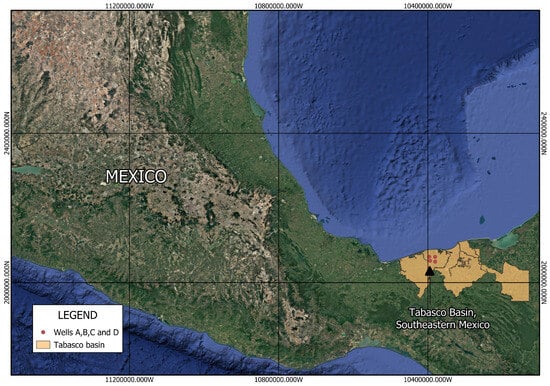
Figure 1.
Simplified location map of the study area within the Tabasco Basin, southeastern Mexico. Red circles mark the approximate well locations used in this study; boundaries are generalized to preserve confidentiality. The basin outline and main structural features are adapted from PEMEX and published sources.
Log availability varies by well and includes, in different combinations, caliper, gamma ray (GR), spontaneous potential (SP), resistivity, neutron porosity (NPHI), bulk density (RHOB), and sonic (DT). Measurements were acquired at a constant sampling interval of 0.15 m (15 cm).
The analyzed wells penetrate interbedded sandstone and shale sequences belonging to the upper Paleogene–Neogene formations of the Tabasco Basin, locally transitioning to carbonate layers toward the southeast. The alternation between clean sands and shaly intervals influences both resistivity and acoustic velocity, providing a suitable setting to test multi-log predictive models.
According to the provider, the logs had already undergone routine vendor corrections; we therefore worked directly with the delivered LAS files. Because the learning task is to predict the sonic log, only wells containing DT could be used for supervised training and evaluation. Of the available wells, six contain DT; four of these share a common set of predictor logs (GR, resistivity, NPHI, and Density) in addition to DT. For confidentiality, we refer to these four wells as A–D, and they constitute the core dataset used for model development and well-level validation.
Two additional wells contain DT but lack one or more of the predictor logs listed above; they are used only in experiments where reduced input sets are evaluated. Wells without DT are reserved for field deployment of the trained models to generate synthetic sonic logs.
Table 3 shows a summary of the available well logs and their usage in the study approach.
Table 3.
Usage of the available well logs.
To prevent information leakage across depths within a borehole, all experiments adopt strict well-level splits: training is performed on a subset of wells, while validation and testing use the remaining wells. Windows are generated only after the well-level split. For the four DT wells that share all predictors, we employ leave-one-well-out cross-validation: three wells are used for training and one for testing, with results averaged across folds. One fold is additionally used for hyperparameter tuning.
Subsequent sections describe preprocessing steps (depth alignment, QC masks, and normalization) and the alternative input configurations evaluated.
4. Methods
4.1. Preprocessing
We worked with LAS-format well logs sampled every 0.15 m (15 cm). Vendor corrections had already been applied. Prior to modeling, we performed geoscience-aware quality control and normalization:
- Outliers and flags: Obvious tool-failure values were masked, and suspect intervals (e.g., washouts) were visually inspected across all logs. Values were removed only when the anomaly was inconsistent with the multi-log context.
- Depth alignment: Each log was resampled onto a common 0.15 m depth grid per well. Minor misalignments between tools—typically on the order of a few centimeters—were corrected by linear interpolation so that corresponding measurements (e.g., GR, NPHI, Density) referred to the same depth levels. This process eliminates artificial phase shifts that could otherwise distort the multilog relationships.
- Resistivity stabilization: Because resistivity values (R) span several orders of magnitude and occasionally contain zero or negative artifacts (from tool noise or vendor flagging), a small positive constant ( m) was added before applying the natural logarithmic transform, i.e.,This prevents undefined values during the logarithmic scaling while preserving the overall distribution. The transformation compresses extreme high values and reduces skewness, facilitating more stable optimization during training.
- Windowing: To provide local depth context and stabilize training, each well was divided into overlapping windows of 200 samples (≈30 m) with 4-sample overlap. Windows containing >10% masked samples were discarded. Windows were shuffled only within the training set.
- Leakage control: All preprocessing steps involving fitted statistics (means, SDs, imputers) were computed on training wells and then applied to validation/test wells.
Figure 2 is the workflow that summarizes the preprocessing performed.
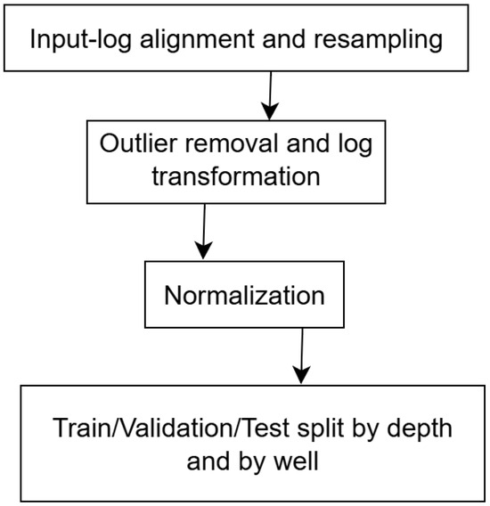
Figure 2.
Preprocessing workflow showing key steps: (1) input-log alignment and resampling, (2) outlier removal and log transformation, (3) normalization, and (4) train/validation/test split by depth and by well. This sequence ensures consistent input preparation prior to model training.
Exploratory scatter plots confirmed nonlinear dependencies between the sonic target and predictors (GR, resistivity, NPHI, RHOB). Figure 3 and Figure 4 illustrate these relationships before and after natural logarithmic-transformation.
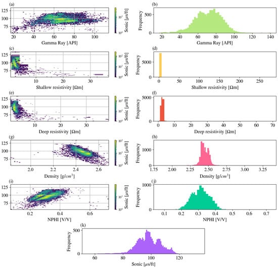
Figure 3.
Nonlinear dependencies between sonic and predictor logs using density heatmaps (a,c,e,g,i) and histograms (b,d,f,h,j,k). (a) Sonic vs. gamma ray; (b) gamma-ray histogram; (c) sonic vs. log(shallow resistivity); (d) histogram of log(shallow resistivity); (e) sonic vs. log(deep resistivity); (f) histogram of log(deep resistivity); (g) sonic vs. density (RHOB); (h) density histogram; (i) sonic vs. NPHI; (j) NPHI histogram; (k) sonic histogram. Heatmap color indicates sample density (log-scaled). All panels combine data from all wells (A–D).
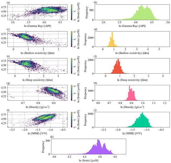
Figure 4.
Nonlinear dependencies between the logarithmically transformed sonic and predictor logs using two-dimensional density heatmaps and histograms. (a) ln (Sonic) versus ln(Gamma Ray) showing the inverse relationship between velocity and clay content. (b) Histogram of ln (Gamma Ray). (c) ln (Sonic) versus ln (Shallow Resistivity) illustrating increasing velocity with higher resistivity. (d) Histogram of ln (Shallow Resistivity). (e) ln (Sonic) versus ln (Deep Resistivity) highlighting compaction-related trends. (f) Histogram of ln (Deep Resistivity). (g) ln (Sonic) versus ln (Density) demonstrating the negative correlation between density and slowness. (h) Histogram of ln (Density). (i) ln (Sonic) versus ln (NPHI) showing the expected direct relation between porosity and slowness. (j) Histogram of ln (NPHI). (k) Histogram of ln (Sonic). Heatmap color indicates sample density (ln-scaled). All panels combine data from all wells (A–D).
4.2. Neural Network Architecture
The convolutional layers used a kernel size of 3, corresponding to a physical window of ≈0.45 m, sufficient to capture local depth trends in well logs while minimizing smoothing. Two stacked GRU layers were employed to encode sequential dependencies in depth without excessive parameter growth. Dropout () was applied after each dense layer to regularize the model; higher values caused underfitting, while lower ones increased validation loss variance. We evaluated a sequence model that combines local feature extraction with longer-range depth dependence:
- Convolutional front-end (feature extractor): Three 1-D convolutional layers along depth with 32, 64, and 64 filters and kernel sizes of 3, 7, and 14 samples, respectively. Stride = 1, same padding, ReLU activations, no pooling. Input logs are stacked as channels.
- Recurrent backbone (context): Two bidirectional gated recurrent unit (GRU) layers with 32 and 64 units, using tanh activations to capture sequential dependence along depth.
- Fully connected head (regression): Dense layers of 32 → 64 → 1 units; hidden tanh activations and linear activation at the output to predict continuous sonic values.
- Regularization: Dropout (rate = 0.2) after each block and weight decay = on dense layers.
- Implementation: TensorFlow/Keras.
Figure 5 shows the implemented neural network architecture.
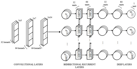
Figure 5.
Schematic of the hybrid CNN–GRU network architecture. Convolutional layers extract local spatial patterns from multi-log inputs; GRU layers capture sequential depth dependencies; dense layers map combined features to the predicted sonic () output.
To assess the role of different predictors, three input configurations were tested:
- 5R model includes all five logs (Gamma Ray, Resistivity, Neutron Porosity, Bulk Density, and Sonic);
- 4R model excludes one log (uses Gamma Ray, Resistivity, Neutron Porosity, and Bulk Density);
- 2R model uses only Gamma Ray and Resistivity as predictors.
These shorthand labels (5R, 4R, 2R) are used throughout Section 5 to refer to the respective input combinations.
4.3. Baselines
We compared the network against widely used baselines:
- Empirical relations: Faust-type velocity–resistivity–depth relation; Gardner and Lindseth density–velocity relations. Constants (a, b, m) were fitted by least squares on training wells.
- Linear/Multi-linear regression: Ordinary least squares (OLS) mapping from predictor logs to sonic. The same input sets as above were tested.
4.4. Training and Evaluation
- Loss and optimizer: Huber loss with (in normalized units) to reduce sensitivity to outliers. Optimizer Adam with initial learning rate = and cosine decay. Weight decay = .
- Batching: Mini-batches of 64 windows.
- Early stopping: Validation loss monitored with patience = 20 epochs; maximum 200 epochs; best weights restored.
- Metrics: Root mean square error (RMSE, in s/ft), mean absolute percentage error (MAPE, in%), mean absolute error (MAE, in s/ft), and coefficient of determination (). Metrics are reported per well and as aggregated mean ± standard deviation.
4.5. Ablations and Sensitivity
Targeted experiments were performed to test robustness:
- Input importance: Compare Full, Reduced-A, and Reduced-B configurations.
- Window length: 100, 200, and 300 samples to test receptive-field sensitivity.
- Normalization: Per-well vs. global z-score (expect per-well to generalize better).
- Loss function: Huber vs. MAE vs. MSE.
- Model variants: MLP-only (no CNN/RNN) and CNN-only (no RNN) to isolate contributions of sequence modeling.
4.6. Statistical Testing
Per-well, test-only errors (RMSE [s/ft] and MAPE [%]) from wells A–D were compared between models using paired Wilcoxon signed-rank tests (two-sided, ) to accommodate the small sample size and potential non-normality. We report mean and median paired differences alongside p-values and n. Boxplots illustrate the per-well error distributions for each model.
5. Results
For clarity, the model acronyms used here refer to their respective input sets: 5R (five logs: GR, Resistivity, NPHI, RHOB, and Sonic), 4R (four logs: GR, Resistivity, NPHI, and RHOB), and 2R (two logs: GR and Resistivity).
5.1. Convergence
All three models (5R, 4R, 2R) converged cleanly. The best validation losses selected by early stopping were (5R), (4R), and (2R), with corresponding training losses of , , and , respectively. The generalization gap is modest for 5R and 4R (≈2.6 and ≈2.4 ) and largest for 2R (≈7.1 ), consistent with the lower information content of its inputs (Figure 6).
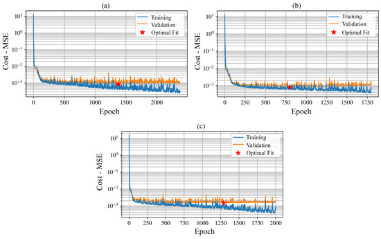
Figure 6.
Training and validation loss versus epoch for the (a) 5R, (b) 4R, and (c) 2R models. Each plot shows the cost function (mean squared error, MSE) evolution during training (blue) and validation (orange) phases, along with the epoch corresponding to the optimal fit (red marker). Panel (a) illustrates the 5R model, which stabilizes rapidly with the lowest generalization gap; panel (b) shows the 4R model, displaying similar convergence but with slightly higher variance;
and panel (c) presents the 2R model, which converges more slowly and exhibits a wider generalization
gap. All models reach stable minima, with the richer architectures (5R and 4R) achieving better
overall performance and smoother validation behavior.
5.2. Held-Out Performance (Within-Well Intervals)
On the held-out test intervals from the four wells used in modeling (A–D), all models achieved low error. Per-well test-only metrics (Table 4) show the following:
- Well A: best RMSE/MAPE from 4R (1.421, 2.02%); 5R is essentially tied (1.427, 2.03%).
- Well B: 5R performs best (1.348, 1.79%).
- Well C: 5R performs best (1.667, 2.98%).
- Well D: 4R performs best (1.211, 1.62%).
Averaged across wells (test-only), the models rank as follows: 5R (RMSE 1.43, MAPE 2.16%), 4R (1.46, 2.23%), and 2R (1.65, 2.81%). In general, richer inputs yield lower error, although 4R occasionally outperforms 5R on specific wells—likely when one of the additional logs introduces noise (Table 4).
Table 4.
Quantitative comparison of predicted versus measured sonic log for wells A–D. This table reports the held-out test intervals only. Lower is better. The 5R model performs best on average, with 4R occasionally superior on individual wells.
Table 4.
Quantitative comparison of predicted versus measured sonic log for wells A–D. This table reports the held-out test intervals only. Lower is better. The 5R model performs best on average, with 4R occasionally superior on individual wells.
| Model 5R | Model 4R | Model 2R | ||||
|---|---|---|---|---|---|---|
| Well Name | RMSE | MAPE | RMSE | MAPE | RMSE | MAPE |
| A-Test | 1.4267 | 2.03% | 1.4212 | 2.02% | 1.6251 | 2.61% |
| B-Test | 1.3483 | 1.79% | 1.4744 | 2.14% | 1.4693 | 2.18% |
| C-Test | 1.6672 | 2.98% | 1.7134 | 3.12% | 1.7995 | 3.44% |
| D-Test | 1.2911 | 1.84% | 1.2108 | 1.62% | 1.7004 | 3.02% |
5.3. Statistical Comparison of Models
We assessed whether performance differences among the three input configurations (5R, 4R, 2R) are statistically meaningful using the per-well, test-only RMSE and MAPE values for wells A–D (Table 4). Because each model was evaluated on the same wells (paired design) and the sample size is small (), paired, non-parametric Wilcoxon signed-rank tests were applied to the model-to-model differences.
Across wells, 5R exhibits the lowest average errors, 4R is close behind, and 2R is consistently worse (Table 5). However, with , the Wilcoxon tests did not reach conventional significance for 5R vs. 4R (RMSE , MAPE ), 5R vs. 2R (RMSE , MAPE ), or 4R vs. 2R (RMSE , MAPE ). Mean paired differences nonetheless favored richer inputs: 5R–2R improved RMSE by 0.22 s/ft and MAPE by 0.65% on average, while 4R–2R improved RMSE by 0.19 s/ft and MAPE by 0.59% (Table 5).
Table 5.
Paired statistical comparison of models using per-well, test-only errors (wells A–D). Negative indicates the first model has a lower error. Reported values are mean and median paired differences across wells, with Wilcoxon signed-rank test statistics and p-values.
Figure 7 shows the per-well distributions (boxplots), highlighting the upward shift and larger dispersion for 2R.
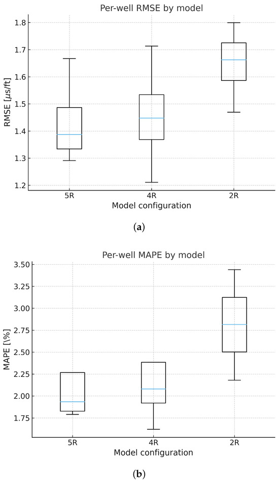
Figure 7.
Per-well RMSE and MAPE by model (test-only). (a) Per-well RMSE by model (test-only).
Each box summarizes the distribution of RMSE across wells A–D for the 5R, 4R, and 2R configurations.
(b) Per-well MAPE by model (test-only). Distributions across wells A–D show higher central tendency
and dispersion for the reduced-input 2R model.
These findings align with the trends reported earlier: richer input sets (5R, 4R) reduce error relative to 2R, while the small number of wells limits statistical power. This limitation is inherent to the dataset design (strict per-well holdouts among the four DT-and-predictor-complete wells) and has already been described in our validation protocol.
Table 6 confirms the overall ranking of models when all intervals are aggregated. Formal statistical comparisons, however, are restricted to the held-out test-only errors in Table 4. Across all depth segments, the ordering remains consistent: 5R (RMSE 1.28, MAPE 1.71%) < 4R (1.34, 1.87%) < 2R (1.43, 2.14%).
Table 6.
Quantitative comparison of predicted versus measured sonic log for wells A–D. This table aggregates train/validation/test segments.
5.4. Depth-Track Case Studies (A–D)
Figure 8 presents overlays of the predicted sonic curves from the 5R, 4R, and 2R models together with the measured sonic curve, restricted to three intervals of well A (the remaining wells appear in Appendix A). Visually, the predictions track lithologic trends closely. Misfits concentrate at sharp facies transitions and thin beds, where limited vertical resolution and log heterogeneities are most pronounced. Dashed brown rectangles highlight the test windows that were not included during training.
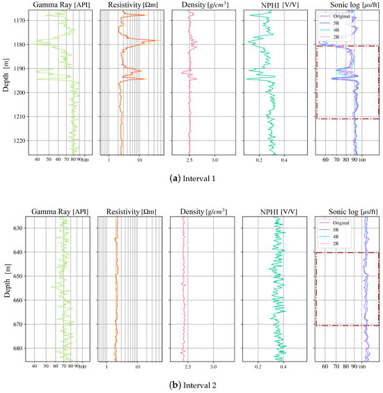
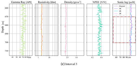
Figure 8.
Sonic-log prediction in well A. Track 5 shows the measured sonic log compared to the model outputs. Brown rectangles indicate test-only intervals.
5.5. Deployment to Wells Without Sonic
We applied the trained models to three additional wells in the same field where sonic was not acquired. When all predictors were present, predictions from 5R, 4R, and 2R were used (shown side-by-side in Figure 9); when only resistivity and gamma were available, 2R was used (Figure 10). The generated sonic logs show consistent stratigraphic trends and are ready for downstream use (synthetic seismograms, mechanical properties).
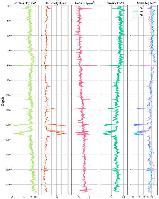
Figure 9.
Prediction sonic in Well X using models five, four, and two input logs (5R/4R/2R).
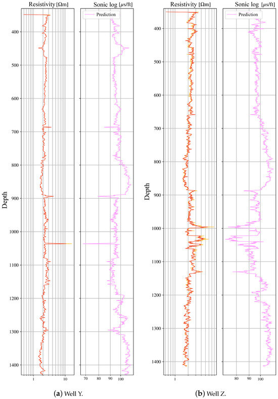
Figure 10.
Predicted sonic in Wells Y and Z using the two-input model (2R) owing to limited log availability.
Table 7 shows the comparison between the proposed ML models (5R,4R,2R) with the empirical and linear-regression baseline in terms of RMSE and MAPE across wells. This quantitative summary complements the figures and highlights the relative improvement achieved by the ML workflow.
Table 7.
Summary of predictive performance for machine-learning and baseline models across test wells.
Because only four wells with complete log suites were available, formal significance testing should be interpreted cautiously. The reported uncertainty ranges therefore reflect inter-well variability rather than population-level statistics.
6. Discussion
The results reveal a consistent agreement between measured and predicted sonic responses across wells with differing lithologies and data completeness. The discussion below links these quantitative metrics (RMSE, MAPE) to geological meaning, highlighting how the model captures stratigraphic variations and assessing its operational usefulness in field interpretation.
6.1. Data Treatment and Sampling Strategy
The log transformation applied to resistivity (and consistently to other inputs) stabilized heavy-tailed distributions while preserving inter-log dependencies. This aided optimization and reduced sensitivity to outliers. Random partitioning into train/validation/test (70/15/15) produced subsets with comparable distributions, indicating a statistically balanced split. However, random depth-wise sampling within wells risks optimistic estimates if neighboring samples leak across subsets. For this reason, results should be interpreted alongside stricter well-level validation, which is the recommended protocol for future work.
6.2. Convergence Behavior and Model Selection
Training followed the expected pattern for Adam: both training and validation losses decreased rapidly, with some stochastic jitter typical of adaptive optimizers. In later epochs, the training loss continued to decline while the validation curve flattened—a classic early sign of overfitting (Figure 6). Selecting checkpoints at the minimum validation loss (with training loss still close) was appropriate and prevented late-epoch drift. “Inspection of predicted sonic curves shows systematic increases in velocity within clean sandstone intervals and pronounced slowdowns in shale-rich layers, consistent with local lithological alternations documented in the Tabasco Basin. These depth-dependent trends suggest that the CNN–GRU network learned meaningful relationships between resistivity, gamma ray, and acoustic velocity that mirror stratigraphic layering. In well B, for example, predicted high-velocity zones coincide with the upper fluvial sandstone unit identified from RHOB and GR logs, confirming the model’s sensitivity to true subsurface changes rather than mere statistical smoothing.”
6.3. What the Metrics Really Say
Using RMSE (in physical units) alongside MAPE (scale-free) provides complementary views. RMSE reports the practical magnitude of errors in [s/ft], while MAPE highlights relative errors that may be masked in absolute units. Taken together, the reported values demonstrate low residuals on held-out intervals and support the case for operational deployment—particularly when predictor coverage is complete.
6.4. Comparing Input Configurations (5R vs. 4R vs. 2R)
Across wells, the 5R and 4R models perform similarly on average, with 5R favored in some wells and 4R outperforming in others. This is consistent with the observation that gamma ray contributes less direct information to sonic than density, neutron porosity, or resistivity in this field. The 2R model (resistivity + gamma) performs worst, as expected, yet still produces acceptable errors on test intervals. Its synthetic tracks reproduce first-order trends where only minimal logs are available. In practice, use 5R when possible, 4R when GR is noisy or absent, and 2R only as a fallback for legacy wells.
Comparison with Empirical Equations
To contextualize the machine-learning performance, we compared the best model (5R) against the empirical baselines. Across the four wells containing sonic data (A–D), the empirical formulas yielded mean RMSE values between 3.4 [s/ft] and 4.1 [s/ft], and mean MAPE between 5.8% and 6.5%. By contrast, the 5R deep-learning model achieved an average RMSE = 1.43 [s/ft] and MAPE = 2.16%, representing an error reduction of roughly 55–60%. The 4R and 2R models also outperformed the empirical approaches, although with smaller margins (≈ 40% and 25%, respectively). These results confirm that the learning-based approach captures nonlinear dependencies between the sonic response and predictor logs that empirical relations cannot, especially in heterogeneous or clay-rich intervals where resistivity–velocity scaling breaks down. The empirical models remain useful as first-order checks, but the neural approach provides a more consistent and geologically realistic reconstruction of the sonic log across wells.
6.5. Operational Value and Limits
Depth-track comparisons between measured and predicted sonic curves (see Figure 8, Figure 9, Figure 10, Figure A1, Figure A2 and Figure A3) show that the model reproduces compaction and stratigraphic patterns inferred from accompanying logs. In intervals where gamma-ray values are low and resistivity is high—conditions typical of cleaner sandstones—the predicted sonic velocities increase, reflecting denser, faster formations. Conversely, low-resistivity, high-gamma intervals, characteristic of shaly units, coincide with lower predicted velocities. These correlations indicate that the model captures geologically meaningful variations rather than purely statistical patterns. The residual mismatches occur mainly near sharp facies transitions or washouts, where borehole conditions degrade data quality. Misfits cluster at sharp facies transitions and in washouts—intervals where borehole effects and thin-bed limits challenge any model. This level of error is acceptable for downstream tasks such as generating synthetic seismograms or screening elastic properties, but users should remain cautious in clay-rich intervals and enlarged-hole zones, where errors and uncertainty increase. Although synthetic sonic logs provide valuable support for seismic-to-well ties and velocity modeling, their use in overpressure or fault-proximal zones carries risk. Misinterpretation of artificially smoothed or biased predictions could underestimate pore-pressure gradients or elastic contrasts, leading to unsafe drilling decisions. We therefore recommend that predicted sonic values be treated as supplementary inputs, validated against offset wells or mud-weight data when used for operational planning. Operationally, the workflow can fill sonic data gaps in real time during log acquisition or well correlation. In fields where sonic tools are unavailable due to borehole conditions, the predicted curves provide provisional velocity models for time–depth conversion and pore-pressure estimation. In the Tabasco Basin, where interbedded shale–sand sequences often cause tool failures, the model’s predictions can guide seismic tie and drilling decisions until measured data are acquired.
6.6. Recommendations for Future Work
Future work should focus on testing this workflow in wells outside the Tabasco Basin to verify transferability. Additional effort should go into incorporating borehole imaging and lithofacies logs to refine feature selection. Using ensemble dropout could help estimate depth-wise uncertainty, and integrating physics-based constraints (e.g., Gardner or Faust relations) would improve interpretability. Collaboration with operators could enable continuous retraining of the model as new field data become available. The following are the most important recommendations for future work.
- Cross-well validation: Implement leave-one-well-out testing to eliminate depth-adjacent data leakage and evaluate transferability.
- Uncertainty quantification: Use Monte Carlo dropout or lightweight ensembles to compute per-depth confidence intervals.
- Lithology-aware inputs: Integrate shale-volume or facies indicators so that similar lithologies cluster in feature space.
- Physics-guided regularization: Introduce soft constraints linking predictions to Gardner- or Lindseth-consistent density–velocity trends.
- Field-transfer calibration: Apply per-well normalization and light fine-tuning when transferring models across basins or logging vendors.
These recommendations summarize specific steps to improve robustness and generalization of the workflow.
Beyond hydrocarbon contexts, predictive log reconstruction has growing relevance in geothermal and mining projects, where sonic or density measurements are often incomplete due to operational constraints. Recent studies [4,44] highlight comparable machine-learning applications for geothermal reservoir characterization and mineralized-zone mapping. The present workflow—emphasizing rigorous preprocessing, uncertainty awareness, and lithology-specific calibration—can therefore serve as a transferable blueprint for other subsurface domains requiring synthetic log generation.
7. Conclusions
This study developed and evaluated a hybrid convolutional–recurrent (CNN + GRU) model for predicting sonic logs in wells from the Tabasco Basin, southeastern Mexico. The workflow incorporated rigorous preprocessing—depth alignment, log normalization, and train–test separation by well—to ensure that model evaluation reflected real operational conditions rather than inter-depth data leakage. The results show that the proposed approach substantially improves accuracy compared with traditional empirical and linear-regression baselines. The best configuration (5R) achieved RMSE = 1.43 ± 0.06 [s/ft] and MAPE = 2.1 ± 0.2%, representing roughly a 55–60% reduction in error relative to Faust- and Gardner-type relations. Predicted sonic profiles reproduced stratigraphic trends consistent with sandstone–shale alternations observed in measured logs, confirming that the model captures true geological variability rather than numerical smoothing. The principal contribution of this work lies in combining local convolutional feature extraction with depth-sequential GRU learning under strict well-level validation, producing a reproducible and interpretable framework for sonic-log reconstruction. Beyond its academic value, the workflow can be directly integrated into petrophysical interpretation and seismic-tie processes, particularly in fields where sonic acquisition is incomplete or technically limited.
Looking forward, the workflow can be extended from research implementation to operational deployment by embedding the trained models into well-log acquisition or petrophysical interpretation platforms. Integration with field data management systems would allow near-real-time generation of synthetic sonic logs in newly drilled wells, reducing dependence on time-consuming laboratory calibrations. Future collaboration with operators could explore transfer learning between basins, routine uncertainty reporting, and automated quality control to facilitate industry-scale adoption.
Key contributions:
- A field-tested pipeline that couples geoscience-aware preprocessing with a compact deep model to predict DT from routinely acquired logs.
- Strict leakage control at both depth and well levels, with performance quantified by RMSE, MAPE, MAE, and (see Table 7), and validated through qualitative depth-track comparisons in Section 6.5 that confirm geological plausibility.
- Operational deployment to wells lacking DT, enabling downstream tasks such as impedance estimation, synthetic seismograms, and rock-mechanics screening where sonic acquisition was skipped.
- Resilience to missing inputs: reduced-input models deliver usable first-order trends, supporting legacy wells and cost-constrained campaigns.
Practical implications:
- The workflow reduces the time and cost associated with running sonic tools in every well and offers a recovery path when logging fails, with immediate benefits for well-to-seismic ties and overpressure screening.
- Synthetic DT fills critical gaps not only in petroleum applications but also in geotechnical and geothermal projects.
Limitations:
- Generalization is currently field-specific: tool vintages, vendor corrections, and lithologic mixes can shift input distributions.
- Errors increase in shale-rich intervals and washouts, where borehole effects and thin beds challenge any method; uncertainty should be explicitly communicated to users.
Future work:
- Lithology/shale awareness: Incorporate a lithology column or shale volume (e.g., learned embeddings) to stabilize predictions across facies boundaries and improve accuracy when some logs are missing.
- Cross-well validation and transfer: Extend evaluation with leave-one-well-out protocols and adopt fine-tuning/domain normalization to transfer models across fields and tool vintages.
- Physics-guided learning: Regularize predictions toward rock-physics relations (e.g., Gardner, Lindseth) or use multi-task objectives (joint DT and RHOB) to encode structure without over-constraining.
- Uncertainty and calibration: Deliver per-depth prediction intervals (e.g., MC-dropout or ensembles) with coverage checks, so end-users can act on quantified risk.
In short, this study shows that data-driven sonic synthesis is operationally viable: it closes acquisition gaps at low cost while remaining faithful to geologic signals. With lithology-aware features, cross-well validation, and calibrated uncertainty, the approach is ready to scale beyond a single field.
Author Contributions
All authors contributed to the study conception and design. Material preparation, data collection, and analysis were performed by J.A.V.-A., J.C.O.-A., S.L.-J., C.C.-C. and A.T.-A. The first draft of the manuscript was written by J.A.V.-A. and all authors commented on the manuscript to update it. All authors have read and agreed to the published version of the manuscript.
Funding
This research received no external funding.
Data Availability Statement
The data presented in this study are available on request from the corresponding author. The data used in this study were obtained from institutions, governmental agencies, and private companies that impose restrictions on their use and distribution. Therefore, access to the dataset is limited in accordance with the confidentiality agreements established by these entities.
Acknowledgments
Sebastian López acknowledges scholarship grant No. 2070474 from SECIHTI.
Conflicts of Interest
The authors declare no conflicts of interest.
Appendix A
Figure A1, Figure A2 and Figure A3 show the remaining wells (B–D) of the predicted sonic curves from the 5R, 4R, and 2R models together with the measured sonic curve, as in Figure 8 for well A; the plots are restricted to three intervals per well.

Figure A1.
Sonic-log prediction in well B. Track 5 shows the measured sonic log compared to the model outputs. Dashed rectangles indicate test-only intervals.

Figure A2.
Sonic-log prediction in well C. Track 5 shows the measured sonic log compared to the model outputs. Dashed rectangles indicate test-only intervals.

Figure A3.
Sonic-log prediction in well D. Track 5 shows the measured sonic log compared to the model outputs. Dashed rectangles indicate test-only intervals.
References
- Lai, J.; Su, Y.; Xiao, L.; Zhao, F.; Bai, T.; Li, Y.; Li, H.; Huang, Y.; Wang, G.; Qin, Z. Application of geophysical well logs in solving geologic issues: Past, present and future prospect. Geosci. Front. 2024, 15, 101779. [Google Scholar] [CrossRef]
- Brie, A.; Endo, T.; Hoyle, D.; Codazzi, D.; Esmersoy, C.; Hsu, K. New Directions in Sonic Logging. Oilfield Rev. 1998, 10, 40–55. [Google Scholar]
- Mirhashemi, M.; Khojasteh, E.R.; Manaman, N.S.; Makarian, E. Efficient sonic log estimations by geostatistics, empirical petrophysical relations, and their combination: Two case studies from Iranian hydrocarbon reservoirs. J. Pet. Sci. Eng. 2004, 45, 123–134. [Google Scholar] [CrossRef]
- Li, Z.; Xia, J.; Liu, Z.; Lei, G.; Lee, K.; Ning, F. Missing sonic logs generation for gas hydrate-bearing sediments via hybrid networks combining deep learning with rock physics modeling. IEEE Trans. Geosci. Remote Sens. 2023, 61, 5921915. [Google Scholar] [CrossRef]
- Ojala, I. Using rock physics for constructing synthetic sonic logs. In Proceedings of the 3rd Canada-US Rock Mechanics Symposium, Toronto, ON, Canada, 9–15 May 2009; Available online: https://geogroup.utoronto.ca/wp-content/uploads/RockEng09/PDF/Session6/4016%20PAPER.pdf (accessed on 13 September 2025).
- Makarian, E.; Mirhashemi, M.; Elyasi, A.; Mansourian, D.; Falahat, R.; Radwan, A.E.; El-Aal, A.; Fan, C.; Li, H. A novel directional-oriented method for predicting shear wave velocity through empirical rock physics relationship using geostatistics analysis. Sci. Rep. 2023, 13, 47016. [Google Scholar] [CrossRef]
- Guntoro, T.; Putri, I.; Bahri, A.S. Petrophysical relationship to predict synthetic porosity log. Search Discov. Artic. 2013, 41124. Available online: https://www.searchanddiscovery.com/documents/2013/41124guntoro/ndx_guntoro.pdf (accessed on 5 September 2025).
- Bader, S.; Wu, X.; Fomel, S. Missing log data interpolation and semiautomatic seismic well ties using data matching techniques. Interpretation 2019, 7, T347–T361. [Google Scholar] [CrossRef]
- Bader, S.; Wu, X.; Fomel, S. Missing well log estimation by multiple well-log correlation. In Proceedings of the 80th EAGE Conference & Exhibition, Copenhagen, Denmark, 11–14 June 2018. [Google Scholar] [CrossRef]
- Lines, L.R.; Alam, M. Synthetic Seismograms, Synthetic Sonic Logs, and Synthetic Core. CREWES. 2012. Available online: https://www.crewes.org/Documents/ResearchReports/2012/CRR201259.pdf (accessed on 20 September 2025).
- Maalouf, E.; Torres-Verdín, C. Inversion-based method to mitigate noise in borehole sonic logs. Geophysics 2018, 83, D61–D71. [Google Scholar] [CrossRef]
- Zhang, D.; Chen, Y.; Meng, J. Synthetic well logs generation via Recurrent Neural Networks. Pet. Explor. Dev. 2018, 45, 629–639. [Google Scholar] [CrossRef]
- Wang, J.; Cao, J.; Fu, J.; Xu, H. Missing well logs prediction using deep learning integrated neural network with the self-attention mechanism. Energy 2022, 261, 125270. [Google Scholar] [CrossRef]
- Saleh, K.; Mabrouk, W.M.; Metwally, A. Machine learning model optimization for compressional sonic log prediction using well logs in Shahd SE field, Western Desert, Egypt. Sci. Rep. 2025, 15, 14957. [Google Scholar] [CrossRef]
- Pham, T.; Tran, T.; Nguyen, H. Missing well log prediction using convolutional long short-term memory network. Geophysics 2020, 85, WA159–WA170. [Google Scholar] [CrossRef]
- Cabello-Solorzano, K.; Ortigosa de Araujo, I.; Peña, M.; Correia, L.; Tallón-Ballesteros, A.J. The impact of data normalization on the accuracy of machine learning algorithms: A comparative analysis. In Proceedings of the 18th International Conference on Soft Computing Models in Industrial and Environmental Applications (SOCO 2023); García Bringas, P., Pérez García, H., Martínez de Pisón, F.J., Martínez-Álvarez, F., Troncoso Lora, A., Herrero, Á., Calvo-Rolle, J.L., Quintián, H., Corchado, E., Eds.; Springer: Berlin/Heidelberg, Germany, 2023; pp. 344–353. [Google Scholar] [CrossRef]
- Kirkham, T. Lasio: Log ASCII Standard (LAS) File Reader for Python. 2023. Available online: https://lasio.readthedocs.io (accessed on 10 January 2025).
- Abadi, M.; Agarwal, A.; Barham, P.; Brevdo, E.; Chen, Z.; Citro, C.; Corrado, G.S.; Davis, A.; Dean, J.; Devin, M.; et al. TensorFlow: Large-Scale Machine Learning on Heterogeneous Systems. 2016. Available online: https://www.tensorflow.org/ (accessed on 24 June 2025).
- Tixier, M.P.; Alger, R.P.; Doh, C.A. Sonic logging. Pet. Trans. AIME 1959, 216, 106–114. [Google Scholar] [CrossRef]
- Glover, P. Sonic Log. University of Leeds. 2016. Available online: https://homepages.see.leeds.ac.uk/~earpwjg/PG_EN/CD%20Contents/GGL-66565%20Petrophysics%20English/Chapter%2016.PDF (accessed on 10 September 2025).
- Serra, O. Fundamentals of Well Logging; Elsevier: Amsterdam, The Netherlands, 1984; Available online: https://books.google.com.mx/books?id=VfXElAEACAAJ (accessed on 27 September 2025).
- Liu, H. Principles and Applications of Well Logging; Springer: Berlin/Heidelberg, Germany, 2017. [Google Scholar] [CrossRef]
- Hacikoylu, P.; Dvorkin, J.; Mavko, G. Resistivity-velocity transforms revisited. Lead. Edge 2006, 25, 1006–1009. [Google Scholar] [CrossRef]
- Halliburton (s.f.). Pseudo Sonic Log ProMax. Halliburton. Available online: https://www.halliburton.com/en/products/geosciences-suite/geophysics-workflow (accessed on 13 September 2025).
- Potter, C.C.; Stewart, R.R. Density predictions using Vp and Vs sonic logs. CREWES Res. Rep. 1998, 10, 1–10. Available online: https://www.crewes.org/Documents/ResearchReports/1998/1998-10.pdf (accessed on 13 September 2025).
- Quijada, M.F.; Stewart, R.R. Density Estimations Using Density-Velocity Relations and Seismic Inversion. CREWES. 2007. Available online: https://www.crewes.org/Documents/ResearchReports/2007/2007-01.pdf (accessed on 13 September 2025).
- Atat, J.G.; Uko, E.D.; Tamunobereton-ari, I.; Eze, C.L. The Constants of Density-Velocity Relation for Density Estimation in Tau Field, Niger Delta Basin. IOSR J. Appl. Phys. 2020, 12, 19–26. [Google Scholar]
- Wyllie, M.R.J.; Gregory, A.R.; Gardner, G.H.F. Elastic wave velocities in heterogeneous and porous media. Geophysics 1956, 21, 41–70. [Google Scholar] [CrossRef]
- Gardner, G.H.F.; Gardner, L.W.; Gregory, A.R. Formation velocity and density—The diagnostic basics for stratigraphic traps. Geophysics 1974, 39, 770–780. [Google Scholar] [CrossRef]
- Mitchell, T.M. Machine Learning; McGraw-Hill: New York, NY, USA, 1997. [Google Scholar]
- Goodfellow, I.; Bengio, Y.; Courville, A. Deep Learning; MIT Press: Cambridge, MA, USA, 2016. [Google Scholar]
- Nie, F.; Hu, Z.; Li, X. An investigation for loss functions widely used in machine learning. Commun. Inf. Syst. 2018, 18, 37–52. [Google Scholar] [CrossRef]
- Ding, B.; Qian, H.; Zhou, J. Activation functions and their characteristics in deep neural networks. In Proceedings of the 2018 Chinese Control and Decision Conference (CCDC), Shenyang, China, 9–11 June 2018; pp. 1836–1841. [Google Scholar] [CrossRef]
- Lau, M.M.; Lim, K.H. Review of adaptive activation function in deep neural network. In Proceedings of the IEEE-EMBS Conference on Biomedical Engineering and Sciences (IECBES), Sarawak, Malaysia, 3–6 December 2018; pp. 686–690. [Google Scholar] [CrossRef]
- Ketkar, N. Deep Learning with Python: A Hands-On Introduction; Apress: New York, NY, USA, 2017. [Google Scholar]
- Zhang, A.; Lipton, Z.C.; Li, M.; Smola, A.J. Dive into Deep Learning; Cambridge University Press: Cambridge, UK, 2023; Available online: https://d2l.ai/ (accessed on 13 September 2025).
- Pascanu, R.; Gulcehre, C.; Cho, K.; Bengio, Y. How to construct deep recurrent neural networks. In Proceedings of the 3rd International Conference for Learning Representations (ICLR), San Diego, CA, USA, 7–9 May 2014. [Google Scholar] [CrossRef]
- Chung, J.; Gulchere, C.; Cho, K.; Benigo, Y. Empirical Evaluation of Gated Recurrent Neural Networks on Sequence Modeling. arXiv 2014, arXiv:1412.3555. [Google Scholar] [CrossRef]
- Shen, G.; Tan, Q.; Zhang, H.; Zeng, P.; Xu, J. Deep learning with gated recurrent unit networks for financial sequence predictions. Procedia Comput. Sci. 2018, 131, 895–903. [Google Scholar] [CrossRef]
- Ruder, S. An overview of gradient descent optimization algorithms. arXiv 2016. [Google Scholar] [CrossRef]
- Kingma, D.P.; Ba, J.L. Adam: A method for stochastic optimization. In Proceedings of the 3rd International Conference for Learning Representations (ICLR), San Diego, CA, USA, 7–9 May 2015. [Google Scholar] [CrossRef]
- Duchi, J.; Hazan, E.; Singer, Y. Adaptive subgradient methods for online learning and stochastic optimization. J. Mach. Learn. Res. 2011, 12, 2121–2159. Available online: https://dl.acm.org/doi/10.5555/1953048.2021068 (accessed on 13 September 2025).
- Hinton, G.; Srivastava, N.; Swersky, K. Overview of mini-batch gradient descent. In Neural Networks for Machine Learning (Lecture 6a); University of Toronto: Toronto, ON, Canada, 2012; Available online: http://www.cs.toronto.edu/~tijmen/csc321/slides/lecture_slides_lec6.pdf (accessed on 13 September 2025).
- Subiatmono, P.; Buntoro, A.; Lukmana, A.H.; David, M.; Kristanto, D. Brittleness prediction using sonic and density logs to determine sweet spot of Brown Shale reservoir. J. Multidiscip. Eng. Sci. Technol. 2022, 9, 15078–15084. [Google Scholar]
Disclaimer/Publisher’s Note: The statements, opinions and data contained in all publications are solely those of the individual author(s) and contributor(s) and not of MDPI and/or the editor(s). MDPI and/or the editor(s) disclaim responsibility for any injury to people or property resulting from any ideas, methods, instructions or products referred to in the content. |
© 2025 by the authors. Licensee MDPI, Basel, Switzerland. This article is an open access article distributed under the terms and conditions of the Creative Commons Attribution (CC BY) license (https://creativecommons.org/licenses/by/4.0/).