Abstract
Accounting for geotechnical property variability is crucial in seismic site response analysis. Traditionally, the influence of each geotechnical property on response parameters is assessed independently. However, this approach limits our understanding of the combined effects of multiple properties on ground response parameters. This study presents a novel, explainable machine learning (ML)-based approach to assess the influence of multiple geotechnical property variations on response parameters. Four ML models, namely AdaBoost, Extreme Gradient Boosting (XGBoost), Random Forest Regressor (RFR) and Gradient Boosting Machine (GBM), were developed for predictive models. The input factors were shear-wave velocity, plasticity index, soil thickness, input motion intensity and unit weight of the soils. The response parameters were peak ground acceleration (PGA) and peak ground displacement (PGD). Multiple statistical performance metrics were computed to evaluate the performance of the models. The results show the superior prediction performance of the GBM model with low error rates and high agreement index (AI), Kling–Gupta efficiency (KGE) and coefficient of determination . The output of the GBM model was further analyzed using Shapley Additive exPlanation (SHAP) technique to explain and identify the most significant factors contributing to the predictions. Finally, the model was used to develop user-friendly web-based software to facilitate rapid predictions of PGA and PGD.
1. Introduction
Earthquake-induced ground motion characterization plays a pivotal role in seismic hazard assessment and structural design. Accurate predictions of ground motion parameters are essential for developing effective safety protocols and ensuring structural resilience. However, the accuracy of these predictions is significantly influenced by geotechnical variability. Accounting for geotechnical variability is critical for improving the reliability of ground motion predictions. The inherent variability within soil profiles represents a key factor that significantly impacts ground motion and must be carefully considered to achieve reliable solutions [1]. A great deal of research has been devoted to evaluating the impact of geotechnical variability on ground motion [2,3,4,5,6,7,8,9]. Many of these variabilities are complex in nature and they primarily stem from various sources of uncertainties related to inherent soil variability, measurement errors and transformation uncertainties, as outlined in the study by Phoon and Kulhawy [10].
Ground motion induced by earthquakes is quantitatively assessed through site response analysis. One-dimensional (1D) equivalent-linear analysis is widely used due to its simplicity and computational efficiency. Traditional seismic site response analyses often evaluate the influence of geotechnical properties on response parameters (e.g., spectral acceleration, amplification factors, peak ground acceleration (PGA), and peak ground displacement (PGD)) separately. For instance, the study by [4] shows that when assessing the impact of shear-wave velocity (Vs) on site response, the shear-wave velocity profile is varied while the nonlinear soil properties and input motion characteristics remain unchanged. This approach enables a clear understanding of how changes in shear-wave velocity affect surface response parameters. Similarly, many previous studies, e.g., [11,12,13,14,15] evaluated the impact of various geotechnical variability on response parameters. In many cases, the variability of Vs is commonly quantified by randomizing the Vs profile using a procedure proposed by Toro [16] while nonlinear soil properties (shear modulus reduction and damping curves) remain unchanged. Similarly, the variability in nonlinear soil properties is evaluated without accounting for variability in Vs or layer thickness. Variability in input motions is evaluated without randomizing Vs or nonlinear soil properties, focusing only on the effects of input ground motion variability, e.g., see [12]. Such univariate analyses may oversimplify the true behavior of geological systems, potentially leading to less accurate risk assessments. Even when all geotechnical properties are varied during site response simulations, interpreting the combined effects of multiple geotechnical variabilities on response parameters remains challenging.
To address these challenges, a promising strategy is to harness the strong explanatory and high predictive power of machine learning (ML) models. The present study employs a multivariate interaction analysis using explainable ML techniques. This approach enables the simultaneous consideration of multiple geotechnical features to predict site response parameters. It represents a significant advancement in seismic risk analysis, aligning with recent trends that emphasize the importance of multivariate and data-driven models for response assessment. In this research, explainable ML algorithms are used to predict peak ground acceleration (PGA) and peak ground displacement (PGD) while evaluating the influence of geotechnical variability; an aspect that cannot be adequately captured through traditional univariate methods. These parameters were chosen due to their critical role in characterizing site response and assessing the seismic hazard impacts on infrastructure. PGA represents the highest acceleration experienced by the ground during an earthquake and serves as a direct indicator of the shaking intensity at a site. This parameter is essential in structural engineering as it influences the design and safety protocols for buildings, bridges, and other critical structures to withstand dynamic loading. On the other hand, PGD quantifies the maximum ground displacement, highlighting the potential for deformation or permanent ground shifts that may occur. PGD is particularly relevant for understanding the impact on long-span structures such as pipelines, railways, and large dams, which are sensitive to displacement. Explainable ML models offer a unique capability to identify the most influential geotechnical properties on these response parameters. Unlike traditional methods, explainable ML models facilitate a more flexible and comprehensive analysis, assessing the contribution of each geotechnical property within the context of the entire feature space.
Thus, this paper aimed to address the following aspects: (1) Develop various ML models for predicting PGA and PGD by accounting for variability of geotechnical properties. (2) Compare the performance and generalization capabilities of developed ML models. (3) Interpret the output of best-performing ML model and rank the input features based on their impact on PGA and PGD predictions using the unified SHAP technique. (4) Deploy the best-performing ML model through a user-friendly software tool.
2. Methods and Dataset
In this section, we will discuss the methodology adopted to develop and evaluate ML models for predicting PGA and PGD. Figure 1 shows a flowchart of the sequential steps undertaken in this study. As shown in the figure, the initial step begins with generating random soil data using Latin Hypercube Sampling (LHS), which is often preferred over simple Monte Carlo sampling due to its efficiency and ability to sample from entire parameter space. Five variables were selected as input features: reference peak ground acceleration (αgR), shear-wave velocity (Vs), soil thickness (H), plasticity index (PI), and unit weight of soil (γ), to develop the models. The selection of input features is based on their well-established relevance to seismic site response assessment. For instance, PI serves as an indirect indicator of soil nonlinearity. In equivalent-linear (EQL) site response evaluations, the stress–strain behavior of soils is commonly represented through modulus reduction and damping curves, which are governed by soil plasticity and other soil properties. These nonlinear characteristics were taken into account by varying PI values within the Darendeli [17] framework.
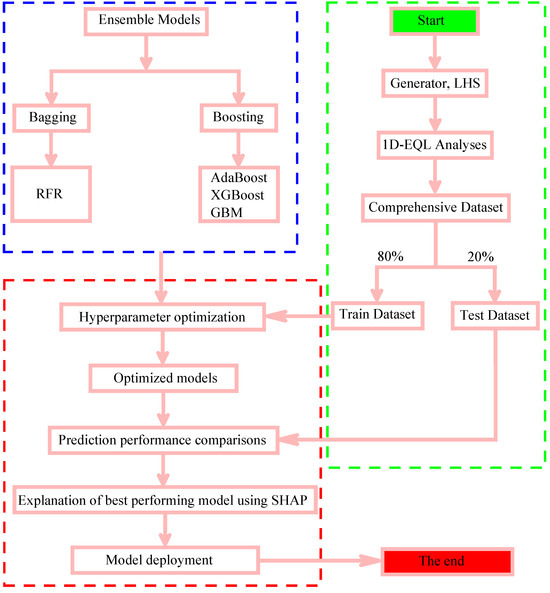
Figure 1.
Flow chart illustrating the methodology adopted in this study.
In reality, some soil properties (e.g., Vs and γ) exhibit correlations with depth or with each other. However, the primary goal of this study was to develop a comprehensive database for training ML models. This approach enables the models to learn from a wide range of soil property combinations, including extreme and less common scenarios, thereby improving their overall generalization capabilities. Consequently, a total of 500 random data points were generated, considering the realistic practical ranges for each input feature. The statistical summary of the generated input feature data is presented in Table 1. The correlation matrix in Figure 2 illustrates the relationships between each feature. Diagonal histograms display the distribution of features, and scatter plots in the lower triangle examine pairwise relationships. The upper triangle shows correlation coefficients, which indicate weak correlations between feature pairs. Using generated input feature data, a series of one-dimensional equivalent-linear (1D-EQL) analyses were conducted with the STRATA software. The primary response parameters obtained from the analyses were PGA and PGD at the ground surface level. The PGA and PGD data were then aggregated with the LHS-generated input features data to create a comprehensive dataset. Subsequently, the dataset was split into a training set (80%) and a test set (20%) to train and evaluate the ML models. For the ML models, the five variables (reference peak ground acceleration, shear-wave velocity, soil thickness, plasticity index, and unit weight of soil) serve as input features while PGA and PGD serve as target variables. The hyperparameters of each model were optimized using a next-generation hyperparameter optimization, Optuna [18] framework. Hyperparameter optimization was performed exclusively on the training set through 5-fold cross-validation. The prediction performance of the optimized models was assessed on the test dataset using various statistical metrics. The best-performing model’s output was further interpreted using SHAP analysis to understand the contribution of each input feature to the predictions. Finally, the model was deployed as a web-based application tool for practical use.

Table 1.
Statistical summary of input features.
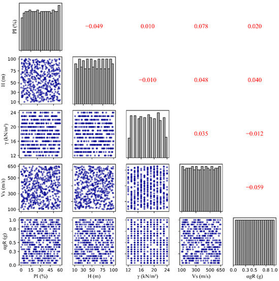
Figure 2.
Correlation matrix plot showing the relationships between input features.
2.1. One-Dimensional Equivalent-Linear (1D-EQL) Analysis
Seismic site response analysis is used to predict ground surface motions for various engineering applications. In most cases, the one-dimensional equivalent-linear (1D-EQL) analysis, proposed by [19], is often the preferred approach owing to its computational efficiency and well-established input parameters. This method simplifies the complex nonlinear problem of soil under seismic loading into an iterative linear process, while retaining acceptable accuracy [20]. The analysis requires careful selection of nonlinear dynamic soil properties, usually represented by normalized shear modulus and damping curves. These properties are typically obtained from laboratory and in situ tests. However, such tests can be resource-intensive, prompting the use of standardized nonlinear material models to approximate soil behavior. Among the widely adopted models, the Darendeli [17] and Vucetic–Dobry [21] nonlinear material models are frequently used in 1D-EQL site response analysis. The Darendeli model integrates essential soil parameters such as the plasticity index (PI), effective vertical stress, and over-consolidation ratio to characterize soil behavior. In this study, the variability of nonlinear soil properties (modulus reduction and damping) was captured by modifying the plasticity index within the Darendeli framework. Consequently, variations in PI serve as a proxy for representing the variability in the nonlinear soil properties.
In the 1D-EQL technique, input motion records (in the form of acceleration time-histories) are applied at the base of the site profile to perform response analysis. Often, these input motion records are selected from ground motion databases that compile real seismic data from monitoring stations worldwide. In this study, records from the Pacific Earthquake Engineering Research Center (PEER) [22] ground motion database were utilized to conduct a series of 1D-EQL response analyses. The Eurocode Type I and Type II spectra (Figure 3) were used as target spectra to identify suitable records in the database [23]. These spectra were customized for reference peak ground acceleration values ranging from 0.05 to 1 g for type A ground conditions. Based on Eurocode 8 [23], type A ground is characterized by Vs greater than 800 m/s. The variation in effectively represents the variability in input motion intensity. Therefore, in this study, the terms “reference peak ground acceleration ()” and “input motion intensity” are used interchangeably. Some of the selected records closely matched the target spectra, while others were scaled to fit the target spectra. Table 2 presents a summary of the input motion records used in this study. The table shows details on the earthquake name and year, faulting mechanisms (e.g., strike-slip, normal, reverse), average shear-wave velocity for the top 30 m (Vs30) of the site, and scale factors applied to the records. The records were then applied at the base of site profiles to compute peak ground acceleration (PGA) and displacement (PGD) at surface level. The statistical summary of obtained PGA and PGD values is presented in Table 3.
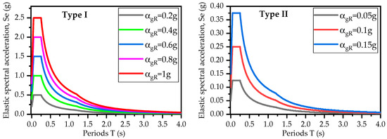
Figure 3.
Eurocode Type I and Type II spectra used as target spectra for record selection.
Table 2.
Summary of input motion records.
Table 3.
Statistical summary of PGA and PGD obtained from site response analyses.
2.2. Machine Learning (ML) Models
ML algorithms have gained substantial attention in predictive modeling across various fields, including geotechnical engineering (e.g., shear-wave velocity prediction [24,25,26,27,28], soil classification [29,30,31,32,33], liquefaction analysis [34,35,36,37], settlement prediction [38,39,40] and stability analysis [41,42]). The models selected for this study included AdaBoost [43], XGBoost [44], Random Forest Regressor (RFR) [45], and Gradient Boosting Machine (GBM) [46]. AdaBoost, introduced by Freund and Schapire, is an ensemble learning technique that combines multiple weak learners to create strong learners [43]. Each weak learner focuses on minimizing the weighted residual errors of previous learners. The final prediction for a regression problem is a weighted sum of the individual weak learners’ outputs. While its effectiveness is widely acknowledged, AdaBoost can be sensitive to noisy data and outliers, which may affect its performance in highly variable datasets. The objective function for AdaBoost can be expressed as follows:
where is the final model, is total number of learners, is the weak learner, and is its corresponding weight.
GBM is another ensemble technique that builds models sequentially, where each new model attempts to correct the errors made by the previous ones [46]. The update rule for GBM can be expressed as follows:
where is prediction at iteration , is a new base learner that minimizes the residuals, and is the learning rate that controls the contribution of each tree.
XGBoost is an advanced and highly optimized implementation of the gradient boosting framework [44]. It is widely recognized for its computational efficiency, scalability, and ability to handle large datasets with high-dimensional feature spaces. In XGBoost, regularization parameter was incorporated to reduce model complexity and prevent overfitting. The objective function of XGBoost is defined as follows:
where is the objective function, is the loss function that measures difference between actual value and predicted value , is the number of observations, is the number of estimators, and is the regularization parameter defined as
where is the number of nodes, is the weight of the leaf nodes, and and are regularization coefficients that control the model’s complexity.
RFR is a bagging-based ensemble algorithm that constructs multiple decision trees during training [45]. Each tree makes predictions, and the final output is obtained by averaging the predictions. The prediction for a new instance can be expressed as
where is the prediction from the tree and is the total number of trees in the forest.
2.3. ML Model Explanation
In the realm of ML, the interpretability of model predictions is paramount, especially as models grow in complexity. In this study, SHapley Additive exPlanations (SHAP) framework, introduced by [47], was used to interpret the output of the best-performing PGA and PGD predictive models. SHAP provides a unified approach to understanding feature importance in these models, enabling a clearer understanding of how input features (in this case, input ground motion intensity , shear-wave velocity , soil thickness , plasticity index , and unit weight of soil influence model outputs (PGA and PGD)). SHAP assigns a unique Shapley value () to each feature based on its contribution to the model output. For a prediction , SHAP is expressed as [47]
where is base value (average model output for the dataset), and is the SHAP value for feature and is defined as follows:
where is the total number of input features, is a subset of features excluding , is the model prediction for the subset , is the number of features in subset , and means that is a subset of the set of features excluding feature . The feature with the highest absolute SHAP value is considered the most influential in the model’s decision-making process.
2.4. Performance Metrics
The performance of each ML model is assessed using several statistical metrics (see Table 4), including root mean squared error (RMSE), mean absolute error (MAE), mean absolute percentage error (MAPE), coefficient of determination (), Index of Agreement (AI), and Kling–Gupta efficiency (KGE) [48,49]. In addition, residual-based prediction intervals were constructed for both PGA and PGD to quantify the predictive uncertainty of each model. The was derived using the standard deviation of residuals obtained from the testing datasets. For each prediction, the 95% prediction interval was calculated around the predicted mean value. These intervals provide an estimate of the range within which the true PGA or PGD values are expected to fall with 95% confidence.
Table 4.
Statistical metrics for evaluating the performance of ML models.
3. Results and Discussions
In this section, the performance of the developed machine learning models (AdaBoost, XGBoost, RFR, and GBM) were thoroughly evaluated. As previously discussed, the hyperparameters of the ML algorithms were optimized using Optuna, taking the root mean squared error (RMSE) as the evaluation metric on the training dataset. For AdaBoost, the optimized hyperparameters include the learning rate, number of estimators, loss function, maximum depth, minimum samples split, and minimum samples per leaf. For XGBoost, the tuning focused on the learning rate, number of estimators, maximum depth, minimum child weight, subsample, and column sample by tree (colsample_bytree). Similarly, the Random Forest Regressor (RFR) was optimized based on the number of estimators, maximum depth, minimum samples split, minimum samples per leaf, and maximum features.
Finally, for Gradient Boosting Machine (GBM), we optimized the learning rate, number of estimators, maximum depth, minimum sample split, minimum samples per leaf, and subsamples. The hyperparameters of each ML algorithm, along with their optimized values, are presented in Table 5 for both PGA and PGD predictive models.
Table 5.
Optuna-optimized hyperparameters of ML models for PGA and PGD predictions.
Table 6 and Figure 4, Figure 5 and Figure 6 illustrate the predictive capabilities of ML models for PGA on both the training and test datasets. The scatter plots of actual versus predicted PGA are presented in Figure 4 for each ML model. The dashed diagonal line (y = x) in each plot represents a perfect agreement between predicted and actual values, whereas the green dashed lines indicate the 95% prediction intervals, defining the range within which predictions are expected to fall with 95% confidence. Among the developed models, RFR and AdaBoost demonstrated the lowest predictive accuracy for PGA on the test and training datasets as can be observed from the spider plots (Figure 5). These two models exhibited relatively high error rates (RMSE, MAE, and MAPE) and lower and KGE values. On the other hand, GBM outperformed the other models for PGA predictions, achieving low error rates and high predictive accuracy. Notably, the GBM model approached ideal predictive performance, yielding IA, and KGE values close to 1. The scatter plots of residuals (differences between predicted and actual values) for PGA are displayed in Figure 6. These plots show that, for both training and testing datasets, the residuals are randomly scattered around the horizontal axis (green dashed line), indicating that each ML model provides unbiased predictions. On the right side of each figure, histograms and probability density curves display the distribution of residuals of the models. The histograms reveal that the residuals are approximately normally distributed and centered around the horizontal axis, indicating a symmetric error distribution, with most predictions close to the actual values and fewer extreme errors. Consistent with statistical metrics, GBM demonstrated exceptional performance, with residuals tightly centered around the horizontal axis and minimal extreme errors. Similarly, Table 7 and Figure 7, Figure 8 and Figure 9 illustrate the predictive capabilities of ML models for PGD across training and test datasets. Consistent with PGA predictive models, the RFR and AdaBoost demonstrated the lower predictive accuracy for PGD, while GBM model outperformed the other models, achieving low error rates and high predictive accuracy. Moreover, the scatter plots of actual vs. predicted PGD (Figure 7) for the GBM model shows clear concentrations along the diagonal line, indicating strong predictive accuracy. Furthermore, the scatter plots of the GBM model residuals (Figure 9) for PGD predictions show that the residuals are tightly centered around the horizontal axis and minimal extreme errors.
Table 6.
Summary of performance metrics for developed PGA prediction models.
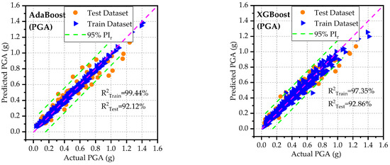
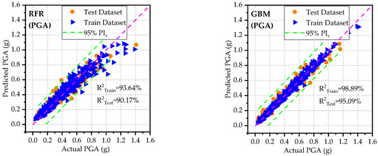
Figure 4.
Actual versus predicted PGA based on developed models for test and training datasets.
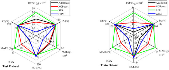
Figure 5.
Comparative performance analysis of models in predicting PGA for test and training datasets.
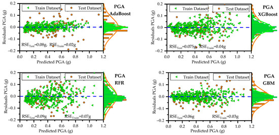
Figure 6.
Scatter plot of residuals showing the distribution of prediction errors for PGA across developed models.
Table 7.
Summary of performance metrics for developed PGD prediction models.
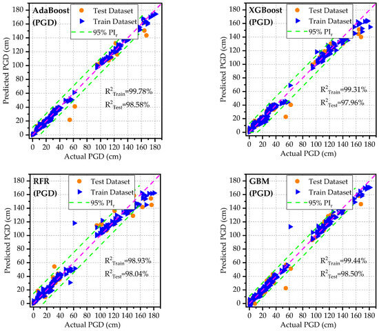
Figure 7.
Actual versus predicted PGD based on developed models for test and training datasets.
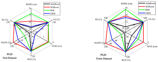
Figure 8.
Comparative performance analysis of models in predicting PGD for test and training datasets.
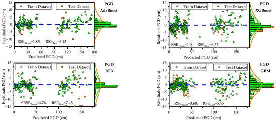
Figure 9.
Scatter plot of residuals showing the distribution of prediction errors for PGD across developed models.
Shap Value
Understanding the impact of key features on the predictive performance of ML models is essential in ground motion analysis. By identifying the most significant features, engineers can make informed decisions regarding ground motion parameters. Therefore, providing clear explanations for the results generated by ML models is a critical step in their effective implementation in practice. In this study, we utilized the SHAP method to interpret the outputs of a GBM model.
The SHAP summary plot (Figure 10) illustrates the influence of each feature on ground response parameters (PGA and PGD). In this plot, each point corresponds to a SHAP value associated with a feature and an individual observation within the dataset. The x-axis represents SHAP values, indicating the impact of each feature on the prediction, while the y-axis lists the features in order of importance. Feature values are color-coded, with red indicating higher values and blue indicating lower values. For instance, high values of shear-wave velocity (Vs) and input motion intensity tend to increase ground response parameters. This observation aligns with geotechnical principles, as Vs is a key determinant of soil stiffness and its ability to transmit seismic waves, while higher input motion intensity corresponds to greater seismic energy input, leading to increased ground motion. Based on their significance and influence on response parameters, the factors affecting PGA (Figure 10a) are ranked as follows: shear-wave velocity > input motion intensity > soil thickness > plasticity index > soil unit weight. For PGD (Figure 10b), the order is as follows: input motion intensity > shear-wave velocity > soil thickness > plasticity index > soil unit weight.
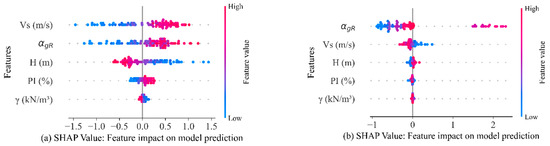
Figure 10.
Beeswarm plot summarizing the global impact of input features using SHAP analysis for (a) PGA and (b) PGD.
The overall importance of each feature is determined by averaging its absolute Shapley values across the entire dataset. These averages are then ranked and displayed in descending order of importance, as shown in Figure 11. A feature with the highest absolute SHAP value is considered the most impactful factor influencing the prediction of GBM. For PGA (Figure 11a), soil shear-wave velocity is identified as the most influential feature, while for PGD (Figure 11b), input motion intensity emerges as the most influential feature. Soil layer thickness () ranks third in importance for both PGA and PGD, indicating its role in modulating wave amplification and energy dissipation through soil strata. The plasticity index () and unit weight () show lower overall importance but still contribute meaningfully to the models’ predictions.
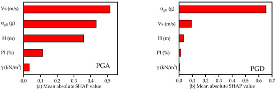
Figure 11.
Global importance of the input features for (a) PGA and (b) PGD.
These findings confirmed that PGA and PGD are dominated by different controlling factors. PGA is primarily governed by Vs, which determines the amplification of high-frequency components of motion. Sites with higher Vs values tend to exhibit greater PGA because stiffer soils more effectively transmit and amplify short-period motions. In contrast, PGD is more sensitive to the intensity and duration of input ground motions, which induce larger cyclic strains. As input motion intensity increases, soils experience greater modulus degradation and damping, dissipating high-frequency energy and reducing PGA while allowing larger cumulative deformation and thus higher PGD. Similar observations were reported by Che et al. [50], who found that prolonged and intense shaking leads to increased strain accumulation in softer deposits.
For the practical implementation of the model, a user-friendly software tool was developed based on the best-performing model (in this case, the Gradient Boosting Machine, GBM model). The graphical user interface (GUI) for the software is shown in Figure 12 and is accessible at https://github.com/Ayele-Tesema/PGA_PGD_Predictor (accessed on 15 October 2025). The model provides rapid predictions of PGA and PGD based on user-input values for the features , , , , and . For instance, entering values of 15% for , 30 m for , 19.5 kN/m3 for , 425 m/s for , and 0.25 g for yields predicted PGA and PGD values of 0.448 g and 5.275 cm, respectively. The 95% prediction interval for PGA is 0.300–0.565 g, while for PGD it ranges from 0 to 15.59 cm. While the predicted values represent the most probable estimates, the prediction intervals quantify the uncertainty associated with model predictions at a 95% confidence level. This information is particularly important in geotechnical engineering, where variability in soil properties and ground motion parameters can significantly influence engineering decisions. Predictions are generated when the “Predict” button is clicked. For the same input feature values, a 1D-EQL analysis using STRATA software produced PGA and PGD values of 0.47 g and 5.25 cm, respectively, demonstrating the effectiveness and reliability of the developed tool in providing comparable results.
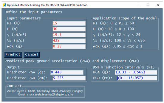
Figure 12.
The graphical user interface (GUI) of software created for PGA and PGD predictions.
It is important to recognize that the dataset utilized in this study was generated through LHS combined with 1D-EQL simulations. For these simulations, input ground motions were selected and scaled to meet Eurocode Type I and Type II target spectra, which introduce an element of simplification. Additionally, the response analyses incorporated a simplification in soil layering by averaging layer thicknesses to a single representative value H, rather than modeling the full stratigraphy with variable layer thicknesses. While these modifications are effective for controlled simulation studies, real field data commonly contain higher levels of noise, heterogeneity, and variability. Applying similar preprocessing steps to real field data is required to predict response parameters with quantifiable uncertainty.
4. Conclusions
A great deal of research effort has been devoted to evaluating the effect of various geotechnical properties on ground motion. Traditionally, these studies assess the influence of individual geotechnical parameters on response parameters. However, this approach limits our understanding of the combined effects of multiple variables on ground response parameters. To bridge this gap, the present study establishes an alternative, explainable ML-based multivariate response analysis. This framework represents a major advancement over traditional univariate approaches. This paradigm shift enhances seismic response evaluation by moving beyond isolated parameter assessments toward an integrated, multivariate understanding of ground motion behavior. Accordingly, four ML models, AdaBoost, XGBoost, GBM and RFR, were developed to predict PGA and PGD using five key geotechnical variables.
The hyperparameters of each model were optimized with the next-generation optimization framework, Optuna, to enhance the accuracy of PGA and PGD predictions. The application of explainable ML models enables a more detailed and insightful identification of key factors influencing ground motion analysis. The study utilized a comprehensive database of 500 1D-EQL analyses to develop the ML predictive models. The database of input parameters, namely, plasticity index , shear-wave velocity , soil thickness , reference peak ground acceleration at bedrock level , and soil unit weight , were generated using LHS, taking their practical ranges into account. The SHAP technique was utilized to rank the input parameters and explain their influence on PGA and PGD predictions. Ultimately, this research demonstrates the potential of explainable ML in advancing ground motion analysis, marking a step toward more data-driven, interpretable, and holistic predictive models in earthquake engineering. The following conclusion can be drawn from this study:
- The developed boosting-based ML models demonstrated a high level of accuracy in predicting PGA and PGD, except for the RFM model. Among the developed ML models, GBM emerged as the best-performing model, achieving the highest predictive accuracy and generalization capability. This model was utilized to develop a user-friendly software tool for practical applications.
- The PGA model achieved excellent performance, with an of 95.95%, a KGE of 93.93%, and an IA of 98.92%, all with minimal errors (RMSE = 0.059 g, MAE = 0.041 g, and MAPE = 12.07%). Similarly, the PGD model achieved an of 98.81%, a KGE of 97.17%, and an IA of 99.69%, with errors of RMSE = 4.71 cm and MAE = 2.01 cm on the test dataset. Notably, for both PGA and PGD models, the residuals had the smallest ranges centered around zero for the test dataset.
- The SHAP method was utilized to interpret and explain the outputs of the GBM model, providing insights into the significance of key features influencing the response parameters. For PGA predictions, the feature importance ranked as follows: shear-wave velocity > input motion intensity > soil thickness > plasticity index > soil unit weight. In contrast, for PGD predictions, the feature importance order was as follows: input motion intensity > shear-wave velocity > soil thickness > plasticity index > soil unit weight. These rankings highlight the clear differences in how geotechnical and seismic parameters influence PGA and PGD, underscoring the value of explainable ML techniques in ground motion analysis.
- Overall, the developed ML models demonstrated effectiveness in predicting PGA and PGD. However, the models rely on input ground motion characterized solely by reference peak ground acceleration as a scalar, which simplifies the complex, rich frequency-dependent behavior of seismic signals. Future research should focus on integrating additional ground motion signatures (e.g., spectral accelerations over multiple frequency bands) and incorporating a broader spectrum of ground motion intensity measures to enhance the versatility and applicability of the developed models.
Author Contributions
Conceptualization, A.T.C. and M.M.; methodology, A.T.C.; software, A.T.C.; validation, J.L. and R.R.; writing—original draft preparation, A.T.C. and M.M.; writing—review and editing, J.L., E.K. and R.R.; supervision, J.L., E.K. and R.R.; All authors have read and agreed to the published version of the manuscript.
Funding
This research received no external funding.
Data Availability Statement
The data utilized in this study is openly accessible in the GitHub repository at https://github.com/Ayele-Tesema/PGA_PGD_Predictor/blob/master/model/pData.csv (accessed on 15 October 2025).
Conflicts of Interest
The authors declare no conflicts of interest.
References
- Tran, T.-T.; Salman, K.; Han, S.-R.; Kim, D. Probabilistic Models for Uncertainty Quantification of Soil Properties on Site Response Analysis. ASCE-ASME J. Risk Uncertain. Eng. Syst. Part A Civ. Eng. 2020, 6, 04020030. [Google Scholar] [CrossRef]
- Idriss, I.M. Evolution of the State of Practice. In Proceedings of the International Workshop on the Uncertainties in Nonlinear Soil Properties and Their Impact on Modeling Dynamic Soil Response; Pacific Earthquake Engineering Research Center Richmond: Richmond, CA, USA, 2004. [Google Scholar]
- Barani, S.; De Ferrari, R.; Ferretti, G. Influence of Soil Modeling Uncertainties on Site Response. Earthq. Spectra 2013, 29, 705–732. [Google Scholar] [CrossRef]
- Rathje, E.M.; Kottke, A.R.; Trent, W.L. Influence of Input Motion and Site Property Variabilities on Seismic Site Response Analysis. J. Geotech. Geoenviron. Eng. 2010, 136, 607–619. [Google Scholar] [CrossRef]
- Aladejare, A.E.; Wang, Y. Sources of Uncertainty in Site Characterization and Their Impact on Geotechnical Reliability-Based Design. ASCE-ASME J. Risk Uncertain. Eng. Syst. Part A Civ. Eng. 2017, 3, 04017024. [Google Scholar] [CrossRef]
- Phoon, K.K.; Kulhawy, F.H. Evaluation of Geotechnical Property Variability. Can. Geotech. J. 1999, 36, 625–639. [Google Scholar] [CrossRef]
- Bommer, J.J.; Abrahamson, N.A. Why Do Modern Probabilistic Seismic-Hazard Analyses Often Lead to Increased Hazard Estimates? Bull. Seismol. Soc. Am. 2006, 96, 1967–1977. [Google Scholar] [CrossRef]
- Wang, M.X.; Wu, Q.; Li, D.Q.; Du, W. Numerical-Based Seismic Displacement Hazard Analysis for Earth Slopes Considering Spatially Variable Soils. Soil Dyn. Earthq. Eng. 2023, 171, 107967. [Google Scholar] [CrossRef]
- Wang, M.X.; Li, D.Q.; Liu, Y.; Du, W.Q. Probabilistic Decoupled Approach to Estimate Seismic Rotational Displacements of Flexible Slopes Considering Depth-Dependent Soil Variability. Acta Geotech. 2022, 17, 1551–1567. [Google Scholar] [CrossRef]
- Phoon, K.K.; Kulhawy, F.H. Characterization of Geotechnical Variability. Can. Geotech. J. 1999, 36, 612–624. [Google Scholar] [CrossRef]
- Rathod, G.W.; Rao, K.S.; Gupta, K.K. Monte Carlo Simulation for Modelling Uncertainties in Ground Response Analysis. Jpn. Geotech. Soc. Spec. Publ. 2015, 2, 709–714. [Google Scholar] [CrossRef]
- Chala, A.; Ray, R. Impact of Randomized Soil Properties and Rock Motion Intensities on Ground Motion. Adv. Civ. Eng. 2024, 2024, 9578058. [Google Scholar] [CrossRef]
- Sun, Q.; Guo, X.; Dias, D. Evaluation of the Seismic Site Response in Randomized Velocity Profiles Using a Statistical Model with Monte Carlo Simulations. Comput. Geotech. 2020, 120, 103442. [Google Scholar] [CrossRef]
- Tran, T.T.; Han, S.R.; Kim, D. Effect of Probabilistic Variation in Soil Properties and Profile of Site Response. Soils Found. 2018, 58, 1339–1349. [Google Scholar] [CrossRef]
- Bazzurro, P. Ground-Motion Amplification in Nonlinear Soil Sites with Uncertain Properties. Bull. Seismol. Soc. Am. 2004, 94, 2090–2109. [Google Scholar] [CrossRef]
- Toro, G.R. Probabilistic Models of Site Velocity Profiles for Generic and Site-Specific Ground-Motion Amplification Studies. Tech. Rep 1995, 779574. [Google Scholar]
- Darendeli, M.B. Development of a New Family of Normalized Modulus Reduction and Material Damping Curves; The University of Texas at Austin: Austin, TX, USA, 2001; ISBN 0493366970. [Google Scholar]
- Akiba, T.; Sano, S.; Yanase, T.; Ohta, T.; Koyama, M. Optuna: A Next-Generation Hyperparameter Optimization Framework. In Proceedings of the ACM SIGKDD International Conference on Knowledge Discovery and Data Mining; ACM: New York, NY, USA, 2019; pp. 2623–2631. [Google Scholar]
- Idriss, I.M.; Seed, H.B. Seismic Response of Horizontal Soil Layers. J. Soil Mech. Found. Div. 1968, 94, 1003–1031. [Google Scholar] [CrossRef]
- Hatheway, A.W. Geotechnical Earthquake Engineering. Environ. Eng. Geosci. 1997, III, 158–159. [Google Scholar] [CrossRef]
- Vucetic, M.; Dobry, R. Effect of Soil Plasticity on Cyclic Response. J. Geotech. Eng. 1991, 117, 89–107. [Google Scholar] [CrossRef]
- Ancheta, T.D.; Darragh, R.B.; Stewart, J.P.; Seyhan, E.; Silva, W.J.; Chiou, B.S.-J.; Wooddell, K.E.; Graves, R.W.; Kottke, A.R.; Boore, D.M. NGA-West2 Database. Earthq. Spectra 2014, 30, 989–1005. [Google Scholar] [CrossRef]
- Code, P. Eurocode 8: Design of Structures for Earthquake Resistance—Part 1: General Rules, Seismic Actions and Rules for Buildings; British Standard: London, UK, 2005. [Google Scholar]
- Olayiwola, T.; Tariq, Z.; Abdulraheem, A.; Mahmoud, M. Evolving Strategies for Shear Wave Velocity Estimation: Smart and Ensemble Modeling Approach. Neural Comput. Appl. 2021, 33, 17147–17159. [Google Scholar] [CrossRef]
- Akhundi, H.; Ghafoori, M.; Lashkaripour, G. Prediction of Shear Wave Velocity Using Artificial Neural Network Technique, Multiple Regression and Petrophysical Data: A Case Study in Asmari Reservoir (SW Iran). Open J. Geol. 2014, 04, 303–313. [Google Scholar] [CrossRef]
- Taheri, A.; Makarian, E.; Manaman, N.S.; Ju, H.; Kim, T.H.; Geem, Z.W.; Rahimizadeh, K. A Fully-Self-Adaptive Harmony Search GMDH-Type Neural Network Algorithm to Estimate Shear-Wave Velocity in Porous Media. Appl. Sci. 2022, 12, 6339. [Google Scholar] [CrossRef]
- Tsiaousi, D.; Travasarou, T.; Drosos, V.; Ugalde, J.; Chacko, J. Machine Learning Applications for Site Characterization Based on CPT Data. In Geotechnical Earthquake Engineering and Soil Dynamics V; American Society of Civil Engineers: Reston, VA, USA, 2018; pp. 461–472. [Google Scholar]
- Assaf, J.; Molnar, S.; El Naggar, M.H. CPT-Vs Correlations for Post-Glacial Sediments in Metropolitan Vancouver. Soil Dyn. Earthq. Eng. 2023, 165, 107693. [Google Scholar] [CrossRef]
- Carvalho, L.O.; Ribeiro, D.B. Soil Classification System from Cone Penetration Test Data Applying Distance-Based Machine Learning Algorithms. Soils Rocks 2019, 42, 167–178. [Google Scholar] [CrossRef]
- Eyo, E.; Abbey, S. Multiclass Stand-Alone and Ensemble Machine Learning Algorithms Utilised to Classify Soils Based on Their Physico-Chemical Characteristics. J. Rock Mech. Geotech. Eng. 2022, 14, 603–615. [Google Scholar] [CrossRef]
- Aydın, Y.; Işıkdağ, Ü.; Bekdaş, G.; Nigdeli, S.M.; Geem, Z.W. Use of Machine Learning Techniques in Soil Classification. Sustainability 2023, 15, 2374. [Google Scholar] [CrossRef]
- Carvalho, L.O.; Ribeiro, D.B. A Multiple Model Machine Learning Approach for Soil Classification from Cone Penetration Test Data. Soils Rocks 2021, 44, e2021072121. [Google Scholar] [CrossRef]
- Chala, A.T.; Ray, R. Assessing the Performance of Machine Learning Algorithms for Soil Classification Using Cone Penetration Test Data. Appl. Sci. 2023, 13, 5758. [Google Scholar] [CrossRef]
- Demir, S.; Sahin, E.K. An Investigation of Feature Selection Methods for Soil Liquefaction Prediction Based on Tree-Based Ensemble Algorithms Using AdaBoost, Gradient Boosting, and XGBoost. Neural Comput. Appl. 2023, 35, 3173–3190. [Google Scholar] [CrossRef]
- Demir, S.; Şahin, E.K. Liquefaction Prediction with Robust Machine Learning Algorithms (SVM, RF, and XGBoost) Supported by Genetic Algorithm-Based Feature Selection and Parameter Optimization from the Perspective of Data Processing. Environ. Earth Sci. 2022, 81, 459. [Google Scholar] [CrossRef]
- Samui, P.; Sitharam, T.G. Machine Learning Modelling for Predicting Soil Liquefaction Susceptibility. Nat. Hazards Earth Syst. Sci. 2011, 11, 1–9. [Google Scholar] [CrossRef]
- Jas, K.; Dodagoudar, G.R. Explainable Machine Learning Model for Liquefaction Potential Assessment of Soils Using XGBoost-SHAP. Soil Dyn. Earthq. Eng. 2023, 165, 107662. [Google Scholar] [CrossRef]
- Nejad, F.P.; Jaksa, M.B. Load-Settlement Behavior Modeling of Single Piles Using Artificial Neural Networks and CPT Data. Comput. Geotech. 2017, 89, 9–21. [Google Scholar] [CrossRef]
- Nejad, F.P.; Jaksa, M.B.; Kakhi, M.; McCabe, B.A. Prediction of Pile Settlement Using Artificial Neural Networks Based on Standard Penetration Test Data. Comput. Geotech. 2009, 36, 1125–1133. [Google Scholar] [CrossRef]
- Chen, R.; Zhang, P.; Wu, H.; Wang, Z.; Zhong, Z. Prediction of Shield Tunneling-Induced Ground Settlement Using Machine Learning Techniques. Front. Struct. Civ. Eng. 2019, 13, 1363–1378. [Google Scholar] [CrossRef]
- Wang, L.; Wu, C.; Tang, L.; Zhang, W.; Lacasse, S.; Liu, H.; Gao, L. Efficient Reliability Analysis of Earth Dam Slope Stability Using Extreme Gradient Boosting Method. Acta Geotech. 2020, 15, 3135–3150. [Google Scholar] [CrossRef]
- Bharti, J.P.; Mishra, P.; Moorthy, U.; Sathishkumar, V.E.; Cho, Y.; Samui, P. Slope Stability Analysis Using Rf, Gbm, Cart, Bt and Xgboost. Geotech. Geol. Eng. 2021, 39, 3741–3752. [Google Scholar] [CrossRef]
- Freund, Y.; Schapire, R.E. A Decision-Theoretic Generalization of On-Line Learning and an Application to Boosting. J. Comput. Syst. Sci. 1997, 55, 119–139. [Google Scholar] [CrossRef]
- Chen, T.; Guestrin, C. Xgboost: A Scalable Tree Boosting System. In Proceedings of the 22nd Acm Sigkdd International Conference on Knowledge Discovery and Data Mining, San Francisco, CA, USA, 13–17 August 2016; pp. 785–794. [Google Scholar]
- Breiman, L. Random Forests. Mach. Learn. 2001, 45, 5–32. [Google Scholar] [CrossRef]
- Friedman, J.H. Greedy Function Approximation: A Gradient Boosting Machine. Ann. Stat. 2001, 29, 1189–1232. [Google Scholar] [CrossRef]
- Lundberg, S. A Unified Approach to Interpreting Model Predictions. arXiv 2017, arXiv:1705.07874. [Google Scholar] [CrossRef]
- Willmott, C.J. On the Validation of Models. Phys. Geogr. 1981, 2, 184–194. [Google Scholar] [CrossRef]
- Gupta, H.V.; Kling, H.; Yilmaz, K.K.; Martinez, G.F. Decomposition of the Mean Squared Error and NSE Performance Criteria: Implications for Improving Hydrological Modelling. J. Hydrol. 2009, 377, 80–91. [Google Scholar] [CrossRef]
- Che, W.; Wang, W.; Chen, Z.; Ye, S. Assessing the Effect of Input Motion Duration on Seismic Site Responses of Layered Soil Deposits Using Spectrally Equivalent Records. Soil Dyn. Earthq. Eng. 2024, 177, 108434. [Google Scholar] [CrossRef]


Disclaimer/Publisher’s Note: The statements, opinions and data contained in all publications are solely those of the individual author(s) and contributor(s) and not of MDPI and/or the editor(s). MDPI and/or the editor(s) disclaim responsibility for any injury to people or property resulting from any ideas, methods, instructions or products referred to in the content. |
© 2025 by the authors. Licensee MDPI, Basel, Switzerland. This article is an open access article distributed under the terms and conditions of the Creative Commons Attribution (CC BY) license (https://creativecommons.org/licenses/by/4.0/).