Abstract
A seismic hazard can be quantified by using probabilities. Modern seismic forecasting models (e.g., Operational Earthquake Forecasting systems) allow us to quantify the short-term variations in such probabilities. Indeed these probabilities change with time and space, in particular after strong seismic events. However, the short-term seismic hazard could also change during seismic swarms, i.e., a sequence with several small-/medium-sized events. The goal of this work is to quantify these changes, using the Italian Operational Earthquake Forecasting system, and also estimate the variations in the Gutenberg–Richter b-value. We focus our attention on three seismic swarms that occurred in Central Italy in October–November 2023. Our results indicate that short-term variations in seismic hazard are limited, less than an order of magnitude, and also that b-value variations are not significant. Placing our findings in a more general context, we can state that according to currently available models and catalogs, the occurrence of seismic swarms does not significantly affect the short-term seismic hazard.
1. Introduction
Seismic sequences are usually of two types. The first one is the classical “mainshock-aftershock” sequence (MAs), where an initial strong event E1 gives birth to its own progeny of triggered events, generally occurring within the triggering area of the mainshock, from the first generation on. The starting event E1 is usually the largest of the sequence, but it may also happen that a stronger offspring E2 occurs. In such a case, either one simply acknowledges the possibility that an aftershock stronger than the mainshock can occur, or the initial shock E1 is re-labeled as foreshock together with all the events preceding E2, the latter becomes the new mainshock, and all its triggered events represent the new progeny (“foreshock-mainshock-aftershock” sequence type).
The second kind of earthquake sequence is instead named “seismic swarm” (SW), and is characterized by numerous series of small-to-moderate events occurring in a local area within a relatively short period of time.
The definition of both the two types of sequences presents a delicate point, about which there is no clear agreement in the literature. Regarding MAs, the main drawback is related to the fact that there is no general rule to identify an event as a mainshock. The labeling of events as “foreshocks”, “mainshocks” and “aftershocks” is completely subjective and not always accepted by the scientific community, since no difference in their physical mechanisms has been proven (e.g., [1]). For example, the most used probabilistic model in statistical seismology, the Epidemic-Type Aftershock Sequence (ETAS) branching process [2,3], distinguishes only between triggered and background events. The latter represents the stationary component of the seismic process, which generates the family of offsprings just because is the first event in time (not the strongest at all). The delicate point in the definition of SWs relies instead on the fact that there is not a precise minimum number of small events for the sequence to be characterized as a swarm type, nor a reference maximum magnitude threshold the events should have. It is also important to stress that, in both cases, it is very difficult to understand into which of the two types an ongoing seismic sequence will evolve; the labeling of MAs or SWs is possible, just a posteriori, after the end of the sequence itself (not to mention the yet non-shared and non-rigid definition of the “end of the sequence” itself).
Another term of comparison between MAs and SWs concerns the seismic hazard in the short term. The need to deliver quasi-real-time earthquake forecasts is becoming more and more important nowadays to help communities prepare for possibly destructive seismic sequences. A leading method in this regard is the probabilistic approach, which allows us to quantify how likely the occurrence rate of events in a given space–time–magnitude domain will be. Operational Earthquake Forecasting (OEF [4]) systems have been developed in several countries worldwide (e.g., Italy [5]; New Zealand [6]; United States [7]; Israel [8]) to produce these short-term probabilities in real time, thus allowing us to highlight (and interpret) their evolution in space and time. More precisely, OEF systems regularly (e.g., daily) deliver the forecast of earthquakes over a specific spatiotemporal window of interest (e.g., one week in 0.1° × 0.1° cells) and above a given threshold of magnitude, based on some probabilistic models typically used in statistical seismology, such as ETAS. Evaluating the evolution of the delivered probabilistic forecasts in near-real time may give insights into the difference between MAs and SWs, as well as into how they affect the short-term probabilistic rate. In general, the models used in OEF to date are expected to better catch the spatiotemporal changes in seismicity in the case of MAs, since the occurrence of a strong initial event more easily influences the probabilistic rates by inducing a large increase. However, there is no condition/hypothesis behind the OEF models that would impede the short-term seismic hazard from also changing when SWs occur. In this paper, we contribute to this discussion by investigating how earthquake swarms affect the short-term probabilistic seismic rate in the case of three real seismic sequences in Central Italy. Save for the drawbacks previously discussed, we ascribe all these sequences to the swarm type.
To complement the analysis, we also investigate the effect of earthquake swarms on short-term seismic hazard in terms of the temporal evolution of the b-value parameter of the Gutenberg–Richter frequency magnitude distribution (FMD). The b-value controls the slope of the FMD in a semi-log plot: the larger this parameter, the smaller the proportion of strong shocks with respect to the little ones. Great interest has been shown in the literature about the possibility of interpreting the spatiotemporal variability of the b-value in terms of the physical process, both before the occurrence of a strong event and during an ongoing seismic sequence, thus considering the capability this parameter could have in acting as a proxy for the average stress condition in the crust. A heated debate has been sparked among seismologists on this matter.
On the one hand, anomalies and transient variations in the b-value have been observed both preceding strong shocks (e.g., [9,10]) and during earthquake sequences (e.g., [11,12]), these changes being explained by some evidence of correlation between the b-value and differential stress, material heterogeneity, or fluid diffusion [13,14,15,16]. In light of these results, some authors proposed to analyze temporal changes in the b-value in terms of precursors for an upcoming large event: examples are the traffic light classification by [17] and the combination of ionospheric GPS-TEC data by [18].
On the other hand, high uncertainty is related to the estimation of the b-value, which is indeed prone to several potential sources of bias, such as catalog incompleteness, magnitude binning, and the size of the earthquake catalog [19,20,21,22]. Obviously, a wrong estimation inevitably leads to apparent variations that do not have any real physical meaning.
In this paper, we investigate the temporal evolution of the b-value by considering the weighted likelihood method [23], which bases the estimation of this parameter on the full history of data (likelihood estimation), with positive weights depending on the time lag between the first event in the catalog and all the other events [24]. Uncertainties are also determined by considering the Gaussian confidence interval [25]. This method does not require subjective choices in the estimation procedure, thus allowing us to obtain robust b-value time series that can be properly evaluated in terms of “different effect of MAs and SWs on short-term seismic hazard”.
2. Materials and Methods
2.1. The Seismic Catalog
To study the effect of earthquake swarms on short-term seismic hazards, we focused on three catalogs from Central Italy, the latter being one of the most active seismic areas in this country. More precisely, we considered the events inside circles with a 30 km radius, centered at the geographical coordinates of (1) the municipality of Sora (Frosinone, Lazio region), i.e., Longitude 13.617° and Latitude 41.717°; (2) the municipality of Monte Cavallo (Macerata, Marche, Italy), i.e., Longitude 13.001° and Latitude 42.992°; and (3) the municipality of Lucoli (L’Aquila, Abruzzo, Italy), i.e., Longitude 13.339° and Latitude 42.291°. The temporal interval considered was 1 January 2018–27 November 2023. We also set a maximum depth of 40 km, to overcome issues related to the likely unreliable hypocentral location of deeper events, and a minimum threshold magnitude ML of 1.0. The seismic map is given in Figure 1, along with time vs. magnitude plots. All these three areas experienced strong earthquakes in recent centuries, according to the CPTI15 historical seismic catalog [26].
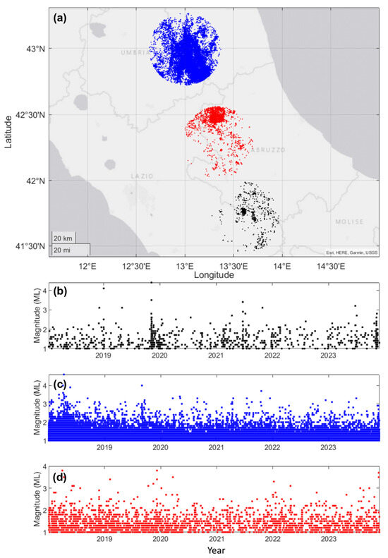
Figure 1.
Panel (a): epicenters of the events considered in this work; black for the Sora catalog, blue for the Monte Cavallo catalog, and red for the Lucoli catalog. Panels (b–d): time vs. magnitude plot for the events in the Sora, Monte Cavallo, and Lucoli catalogs, respectively.
In recent months, these three areas have experienced swarm-like seismic activity, characterized by a high number of events, all with relatively small magnitudes. More precisely, since 1 October 2023, the recorded events with ML 1+ are seventy-eight in the Sora catalog (two events with ML 2.5+, maximum magnitude ML 2.8), three hundred and sixty-three in the Monte Cavallo catalog (five events with ML 2.5+, maximum magnitude two events with ML 2.9) and fifty-nine in the Lucoli catalog (three events with ML 2.5+, maximum magnitude ML 3.7). From Figure 1b–d, it is possible to note an increase in the seismicity in the right part of the plots. Figure 1b shows a huge increase in the number of events, while in the two other zones, this increase is partially masked by the higher background seismicity level.
Since the events’ magnitudes are expected to follow the Gutenberg–Richter frequency distribution [27], we estimated the completeness threshold for the three considered catalogs by means of the Lilliefors test [28,29] for magnitudes’ exponentiality. The determination of the proper completeness magnitude is actually a delicate point to address, as several factors may produce artifacts biasing its estimate and consequently the estimate of the b-value. Several methods have been proposed in the literature to estimate , such as the Maximum Curvature (MaxC) or the 90% and 95% goodness of fit of the FMD to the exponential distribution (e.g., [30,31,32]). However, none of them is specific for testing the exponential property of the magnitudes, well acknowledged in statistical seismology. The canonical statistical test in this scope is the Lilliefors, which is indeed a modification of the classical nonparametric one-sample Kolmogorov–Smirnov, where data are tested for coming from an exponential distribution instead of the classical Gaussian one [28,33]. Despite being less conservative than, for example, the MaxC method, the Lilliefors test allows us to obtain a statistically robust result. Because of the closeness of the three areas, all in Central Italy, and due to the comparable seismic activity, we also stress that we estimated a single completeness magnitude for all the cases, obtaining a value of 1.5.
2.2. The Italian Operational Earthquake Forecasting System
As anticipated in the Introduction, in order to study the evolution of these swarm-type sequences and to investigate potential scenarios after the temporal window of analysis, we followed two main methods. The first one is related to the Operational Earthquake Forecasting (OEF) Italian system [5], which produces real-time short-term earthquake forecasts in each 0.1° × 0.1° cell of a spatial grid covering the entire Italian territory, according to the standards of the Collaboratory for the Study of Earthquake Predictability (CSEP [34]). At midnight every day and after the occurrence of any ML 3.5+ event, the OEF-Italy system delivers the weekly expected rate of events with ML 4+ and 5.5+, with Modified Mercalli Intensity (MMI) VI+, VII+, and VIII+. The forecast is probabilistic and based on the ensemble combination of three models typically used in statistical seismology: the Epidemic-Type Aftershock Sequence (ETAS) proposed by [35], the Epidemic-Type Earthquake Sequence (ETES) by [36], and the Short-Term Earthquake Probability (STEP) by [37]. Common to all these models is the Omori–Utsu law for the temporal decay of aftershocks [38,39] and the decreasing exponential Gutenberg–Richter law for the magnitudes. Both ETAS and ETES belong to the class of self-exciting Hawkes processes of branching type and are based on the rationale that seismic events cluster in space and time and evolve in successive generations independently of the others. Instead, the STEP model first recasts the forecasts in terms of strong ground-shaking probability; then, it combines a time-dependent model of earthquake occurrence, based on faults and historical data, with (i) a Reasenberg and Jones type of clustering model [40], (ii) a sequence-specific model, and (iii) a spatially heterogeneous model. The combination of ETAS, ETES, and STEP is weighted according to the past performance of the three models considered. As input, OEF uses events with ML 2.5+ and is continuously updated according to the catalog recorded by the seismic surveillance system of the INGV. The OEF-Italy system is shown to deliver globally reliable forecasts [41,42], and is therefore the first tool we used in this study to investigate the evolution of the considered swarm-type seismic sequences.
2.3. The Gutenberg–Richter b-Value Estimation
The second method we followed is instead related to the well-known b-value parameter of the Gutenberg–Richter law, which, as anticipated in the Introduction, controls the proportion of larger shocks with respect to the smaller ones. In this paper, we analyzed the temporal variation of the b-value by means of the weighted likelihood method [23], which allowed us to estimate this parameter based on the full history of available data. The weights for the likelihood are defined as in [24]: each weight (i = 1, …, N events) is positive and expressed as an exponential kernel depending on the time lag between the i-th event and the first event in the catalog:
where is a normalizing constant and is a “forgetting parameter”, which quantifies the amount of relevant past information. The parameter is found through a maximum likelihood estimate (MLE) approach.
The weighted likelihood estimation of the b-value, properly corrected to account for magnitudes’ binning (see also [43]), is then obtained as follows:
where are the events’ magnitudes, is the completeness magnitude, and is the magnitude binning (in our case, 0.1). The uncertainty was finally determined by considering the normal approximation, with the b-value standard error σ equal to / [19,25,44]. The difference between the weighted likelihood method and the classical [25] MLE approach is straightforward, with the first approach being a generalization of the latter. In the MLE case, each event has the same importance in the estimation. In the weighted likelihood case, the importance is related to the temporal distance of events used in the estimation: the larger the distance between the time of the event and the actual time ( in Equation (1)), the smaller the importance in the estimation. The advantage of this method is that we do not need subjective choices for the building of the b-value time series: in the classical rolling-window approach, a fixed number of events is used to build the time series (usually 50, 100, or 200), and this number is a subjective decision of the researcher. Here, the parameter , which rules the importance of past information in the estimation of the actual b-value, is estimated through an MLE approach, avoiding subjective choices on the number of events used.
3. Results and Discussion
3.1. OEF Probabilities
The OEF probabilities of MMI VI+, VII+, or VIII+ and ML 4+ or 5.5+ events, for the three areas under analysis, are given in Table 1. Specifically, we report the background rate computed during the last 5 years for each case, together with the maximum peaks of probability since October 2023, as well as the weekly probabilities delivered on the last date considered in our catalogs, i.e., 27 November 2023.

Table 1.
OEF probabilities for the three considered catalogs.
The OEF-Italy graphical interfaces relative to the case ML 5.5+ are also given in Figure S1 of the Supplementary Material (the top, middle, and bottom panels are for the Sora, Monte Cavallo, and Lucoli catalogs, respectively). The results show that, for all the catalogs considered, there is a small increase from the background rates to the highest peaks observed during the swarm activity since October 2023. Precisely, from the zero increase obtained for Monte Cavallo in the cases of MMI VI+ and ML 5.5+, we observe a maximum increase of about four times in the MMI VII+ and MMI VIII+ rates for Lucoli. The latter is indeed the catalog for which the OEF rates are shown to be more influenced by the seismic activity, although very slightly. Interestingly, the swarm sequence in Lucoli is not the one containing the highest number of ML 2.5+ events among the catalogs considered here (we recall that only these events are accounted for, in computing the OEF rate). That is to say, one ML 3.7+ event (as in Lucoli) weighs more than a higher number of smaller events, provided they all have an ML of 2.5+, including two ML 2.9 (as in Monte Cavallo). Finally, Sora shows consistency for the five cases (all rates increase by about 1.5 times).
It is important to stress that, after the occurrence of the strongest events in the three considered areas during the entire operating period of OEF (from 2009), the OEF rates actually increased considerably. Regarding Sora, the maximum peaks were obtained during the 2009 L’Aquila sequence, which indeed also affected this area due to its proximity to the Abruzzo region, and during the 2013 sequence, the rates increased by factors from 20 to 35, reaching, for example, an MMI VIII+ rate of 2 × 10⁻³ and an ML 4+ rate of 0.05. The same sequence induced an increase in the OEF rates relative to Lucoli from two to three orders of magnitude. On 6 April 2009 at 8:00 a.m., OEF released an 80% probability of this area having an ML 4+ event during the following week. A 90% probability was finally released for MMI VI+ and ML 4+ events after the Norcia Mw 6.5 earthquake in the area around Monte Cavallo; here, OEF rates increased by factors from 100 to 250 during the Central Italy sequence. Overall, comparing the OEF maxima probabilities delivered after the strongest events experienced since 2005 with those obtained during the current swarm activity, we observe an increase factor IF from the background that is about 20 times higher for Sora, 60 times higher for Lucoli, until 250 times higher for Monte Cavallo. The factors of increase for all the cases are given in Table S1 of the Supplementary Materials.
In conclusion, we can deduce that the occurrence of a swarm-type sequence does not significantly increase the OEF-Italy system probabilities, and the observed increases are smaller than one order of magnitude (i.e., less than 10 times) with respect to the background probabilities.
3.2. Temporal b-Value Variations
The results of the estimation of the temporal b-value variations from 1 January 2019 to 27 November 2023 are shown in Figure 2. These results show three different situations for the three catalogs. In the case of Sora (Figure 2a), the b-value shows no significant variation for the whole time period. This also reflects the result that this catalog shows, with respect to the other catalogs, the smallest OEF increase factor IF from the background when comparing the maxima probabilities delivered after the strongest events experienced since 2005 with those obtained during the current swarm activity.
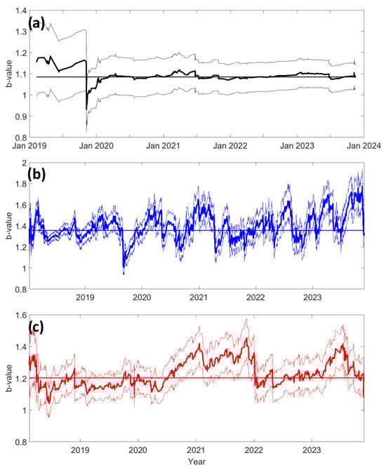
Figure 2.
b-value time series (thick lines), with the associated uncertainty (+/− σ, thin lines), for the Sora catalog (a), the Monte Cavallo catalog (b), and the Lucoli catalog (c). Horizontal lines represent the b-value computed for all catalogs (considered the background value).
Regarding the Monte Cavallo catalog, we have a larger number of events during the analyzed time period, and we can observe a fluctuation in the b-value. In the last month, it is possible to observe a decrease in the b-value; however, this decrease led to the b-value being near the background value (i.e., the value computed using all the events in the complete part of the catalog). Recalling that this parameter is estimated by means of the magnitudes (usually the local ML), the evidence just discussed agrees with the fact that Monte Cavallo shows, for the OEF ML4+ and ML5.5+ rates, an IF∼1 during the current swarm activity and experienced some of the highest IFs after the largest shock (see Table S1 of the Supplementary Materials).
For the Lucoli catalog, we observe moderate fluctuations of the b-value, and generally, these fluctuations are not significantly different from the background value. Also in this case, we can observe a small decrease in the b-value in the last part of the catalog; nevertheless, its decrease is not significant and is constrained within the uncertainty range. Recalling that Lucoli is indeed the catalog for which we observed a slightly higher influence of the swarm activity on the OEF rates, we could have expected to obtain a more evident fluctuation of the b-value in this case. However, we have to recall that Lucoli experienced the lowest number of events during the current swarm activity: 84% and 24% less than in Monte Cavallo and Sora, respectively. Furthermore, it experienced the highest magnitude, i.e., one ML 3.7, which is quite but not significantly higher than the single ML 2.8 and the pair of ML 2.9 that occurred in Sora and Monte Cavallo, respectively. Now, recalling that a sufficient statistic for the b-value estimate is indeed the mean magnitude [19,25,45], it seems reasonable to have obtained variations for this parameter, in the case of Lucoli, which are lower than but comparable to those for Monte Cavallo and slightly higher than for Sora.
In conclusion, the b-value variations for all three catalogs do not show significant deviation from the background value during the seismic swarms of October and November 2023, i.e., estimated values considering the uncertainty are similar to the background value. Overall, the results obtained for the b-value are consistent with those obtained for the OEF rates, in terms of their relative variations. Moreover, since the b-value time series of Monte Cavallo and Lucoli shows general fluctuations in recent years (Figure 2a,b), we underline the difficulty of identifying significant b-value variations in such a type of time series. Statistical b-value fluctuations, not related to any physical phenomena, mask the possible identification of increased/decreased b-value patterns if we have a limited number of events, as in our swarm seismicity case. Therefore, the study of b-value variations of aftershock sequences is clearly different from our situation, since the number of available events is dissimilar, at most hundreds in the swarm case vs. thousands for aftershock sequences.
Finally, we stress that for all the catalogs, the maximum observed magnitude in the considered time period is smaller than ML 4.5; therefore, we do not expect short-term aftershock incompleteness problems related to our 1.5 completeness threshold. We also verified this argument by observing that the sequential number of events shows a homogeneous pattern when plotted versus the magnitudes (heuristic technique [46]; see Figure S2 of the Supplementary Materials). We recall that short-term aftershock incompleteness could lead to a biased estimation of the b-value [22]. For the sake of comparison, we finally performed the estimation of the b-values for the three catalogs by considering also the classical method of a rolling window with a fixed number of 100 events. As expected, results are consistent with those obtained above, but the estimations present a higher volatility (see Figure S3 of the Supplementary Materials).
4. Conclusions
Seismic swarms are characterized by numerous series of small-to-moderate events occurring in a local area within a relatively short period of time. Some of these swarms can lead to strong seismic events, as in the case of the 2009 L’Aquila earthquake in Central Italy (Mw 6.1 [47]). In this work, we analyze the effect of three seismic swarms on the probability released by the Italian Operational Earthquake Forecasting system (OEF) and on the temporal b-value variations. The study of b-value variations is important because its significant decrease could be related to an increase in the probability of a large impending earthquake. Our results highlight how the effect of swarms in OEF is very limited. No matter how many events occur, if they remain “small” (i.e., smaller than 4.0), the increase in the weekly probability of strong events in that area is less than one order of magnitude (i.e., 10 times).
The b-value temporal variations show, for two out of three time series, several fluctuations over recent years. These fluctuations include both increases and decreases in the b-value, making the interpretation of a deviation from the background value during the seismic swarms difficult, and consequently making it impossible to infer something from this parameter.
We can therefore conclude that, although the Central Italy zone is a well-monitored seismic area, with a completeness magnitude of ML 1.5 and with the OEF Italian system operating for more than 10 years, the occurrence of the three studied seismic swarms is not indicative of a significant variation in the probability of large impending events. Since both the OEF system and the studies of b-value variations are similar in other parts of the world, we can generalize our results. Seismic swarms containing about 50–200 events, and with a maximum observed magnitude smaller than 4.0, do not significantly increase the probability of strong impending events for OEF and b-value methodologies.
These findings should push seismologists to find other ways of studying seismic swarms if they want to extract information related to future large events, for example, investigating new spatio-temporal and magnitude statistical relations or using machine or deep learning techniques (e.g., [48,49]). Such techniques adopt optimized methods to reveal the temporal seismic structure, as they are truly trained from data.
Supplementary Materials
The following supporting information can be downloaded at https://www.mdpi.com/article/10.3390/geosciences14020049/s1, Figure S1: OEF probabilities of ML 5.5+ events: top, middle, and bottom panels for Sora, Monte Cavallo, and Lucoli catalogs, respectively; Figure S2: Magnitudes versus sequential number of events: top, middle and bottom panels respectively for Sora, Monte Cavallo and Lucoli catalogs; Figure S3: b-value time series (thick lines), with the associated uncertainty (+/− σ, thin lines), estimated by means of a rolling window with a fixed number of 100 events: panels (a–c) respectively for Sora, Monte Cavallo and Lucoli catalogs; Table S1: Factor of increase in the OEF probabilities for the three considered catalogs, from the background to both the maximum probability during the swarm current activity and the maximum probability after the occurrence of the corresponding past strongest events.
Author Contributions
Conceptualization, I.S. and M.T.; methodology, software, and formal analysis, I.S. and M.T; writing—original draft preparation, I.S.; writing—review and editing, I.S. and M.T. All authors have read and agreed to the published version of the manuscript.
Funding
This research was partially funded by Centro di Pericolosità Sismica (CPS) of INGV, Italy.
Data Availability Statement
Seismic catalog data can be freely accessed on the Istituto Nazionale di Geofisica e Vulcanologia (INGV) website http://terremoti.ingv.it/ (accessed on 15 December 2023).
Acknowledgments
The authors are grateful to the president of the Istituto Nazionale di Geofisica e Vulcanologia (INGV) Carlo Doglioni, and to the the coordinator of the Seismic Hazard Center (Centro di Pericolosità Sismica, CPS, INGV) André Herrero, for the very useful discussion that inspired this study. The authors also thank the Editor-in-Chief, the assistant Editor and the two anonymous reviewers for their useful comments and suggestions that helped to improve the quality of the manuscript.
Conflicts of Interest
The authors declare no conflicts of interest.
References
- Helmstetter, A.; Sornette, D. Foreshocks explained by cascades of triggered seismicity. J. Geophys. Res. Solid Earth 2003, 108. [Google Scholar] [CrossRef]
- Ogata, Y. Statisticals Models for Earthquake Occurrences and Residual Analysis for Point Processes. J. Amer. Statist. Assoc. 1988, 83, 9–27. [Google Scholar] [CrossRef]
- Ogata, Y. Space-time point-process models for earthquake occurrences. Ann. Inst. Stat. Math. 1998, 50, 379–402. [Google Scholar] [CrossRef]
- Jordan, T.H.; Marzocchi, W.; Michael, A.J.; Gerstenberger, M.C. Operational earthquake forecasting can enhance earthquake preparedness. Seismol. Res. Lett. 2014, 85, 955–959. [Google Scholar] [CrossRef]
- Marzocchi, W.; Lombardi, A.M.; Casarotti, E. The establishment of an operational earthquake forecasting system in Italy. Seismol. Res. Lett. 2014, 85, 961–969. [Google Scholar] [CrossRef]
- Christophersen, A.; Rhoades, D.A.; Gerstenberger, M.C.; Bannister, S.; Becker, J.; Potter, S.H.; McBride, S. Progress and challenges in operational earthquake forecasting in New Zealand. In Proceedings of the New Zealand Society for Earthquake Engineering Annual Technical Conference, Wellington, New Zealand, 26 April 2017. [Google Scholar]
- Field, E.H.; Milner, K.R.; Hardebeck, J.L.; Page, M.T.; van der Elst, N.; Jordan, T.H.; Michael, A.J.; Shaw, B.E.; Werner, M.J. A spatiotemporal clustering model for the third Uniform California Earthquake Rupture Forecast (UCERF3-ETAS): Toward an operational earthquake forecast. Bull. Seismol. Soc. Am. 2017, 107, 1049–1081. [Google Scholar] [CrossRef]
- Falcone, G.; Spassiani, I.; Ashkenazy, Y.; Shapira, A.; Hofstetter, R.; Havlin, S.; Marzocchi, W. An operational earthquake forecasting experiment for israel: Preliminary results. Front. Earth Sci. 2021, 9, 729282. [Google Scholar] [CrossRef]
- Chen, X.; Li, Y.; Chen, L. The characteristics of the b-value anomalies preceding the 2004 M w9. 0 Sumatra earthquake. Geomat. Nat. Hazards Risk 2022, 13, 390–399. [Google Scholar] [CrossRef]
- Gunti, S.; Roy, P.; Narendran, J.; Pudi, R.; Muralikrishnan, S.; Kumar, K.V.; Subrahmanyam, M.; Israel, Y.; Kumar, B.S. Assessment of geodetic strain and stress variations in Nepal due to 25 April 2015 Gorkha earthquake: Insights from the GNSS data analysis and b-value. Geod. Geodyn. 2022, 13, 288–300. [Google Scholar] [CrossRef]
- De Gori, P.; Lucente, F.P.; Lombardi, A.M.; Chiarabba, C.; Montuori, C. Heterogeneities along the 2009 L’Aquila normal fault inferred by the b-value distribution. Geophys. Res. Lett. 2012, 39, L15304. [Google Scholar] [CrossRef]
- Montuori, C.; Murru, M.; Falcone, G. Spatial variation of the value observed for the periods preceding and following the 24 August 2016. Amatrice earthquake ML 6.0) (Central Italy). Ann. Geophys. 2016, 59. [Google Scholar] [CrossRef]
- Henderson, J.; Main, I.; Pearce, R.; Takeya, M. Seismicity in North-Eastern Brazil: Fractal clustering and the evolution of the b value. Geophys. J. Int. 1994, 116, 217–226. [Google Scholar] [CrossRef]
- Gerstenberger, M.; Wiemer, S.; Giardini, D. A systematic test of the hypothesis that the b value varies with depth in California. Geophys. Res. Lett. 2001, 28, 57–60. [Google Scholar] [CrossRef]
- Amitrano, D. Brittle-ductile transition and associated seismicity: Experimental and numerical studies and relationship with the b-value. J. Geophys. Res. 2003, 108, 2044. [Google Scholar] [CrossRef]
- Scholz, C. On the stress dependence of the earthquake b-value, Geophys. Res. Lett. 2015, 42, 1399–1402. [Google Scholar] [CrossRef]
- Gulia, L.; Wiemer, S. Real-time discrimination of earthquake foreshocks and aftershocks. Nature 2019, 574, 193–199. [Google Scholar] [CrossRef]
- Nayak, K.; Romero-Andrade, R.; Sharma, G.; Zavala, J.L.C.; Urias, C.L.; Trejo Soto, M.E.; Aggarwal, S.P. A combined approach using b-value and ionospheric GPS-TEC for large earthquake precursor detection: A case study for the Colima earthquake of 7.7 Mw. Mexico. Acta Geod. Geophys. 2023, 58, 515–538. [Google Scholar] [CrossRef]
- Marzocchi, W.; Spassiani, I.; Stallone, A.; Taroni, M. How to be fooled searching for significant variations of the b-value. Geophys. J. Int. 2020, 220, 1845–1856. [Google Scholar] [CrossRef]
- Geffers, G.M.; Main, I.G.; Naylor, M. Biases in estimating b-values from small earthquake catalogues: How high are high b-values? Geophys. J. Int. 2022, 229, 1840–1855. [Google Scholar] [CrossRef]
- Spassiani, I.; Taroni, M.; Murru, M.; Falcone, G. Real time Gutenberg–Richter b-value estimation for an ongoing seismic sequence: An application to the 2022 marche offshore earthquake sequence (ML 5.7 central Italy). Geophys. J. Int. 2023, 234, 1326–1331. [Google Scholar] [CrossRef]
- Lombardi, A.M. Anomalies and transient variations of b-value in Italy during the major earthquake sequences: What truth is there to this? Geophys. J. Int. 2023, 232, 1545–1555. [Google Scholar] [CrossRef]
- Hu, F.; Zidek, J.V. The weighted likelihood. Can. J. Stat. 2002, 30, 347–371. [Google Scholar] [CrossRef]
- Taroni, M.; Vocalelli, G.; De Polis, A. Gutenberg–Richter B-value time series forecasting: A weighted likelihood approach. Forecasting 2021, 3, 561–569. [Google Scholar] [CrossRef]
- Aki, K. Maximum likelihood estimate of b in the formula log N = a-bM and its confidence limits. Bull. Earthq. Res. Inst. Tokyo Univ. 1965, 43, 237–239. [Google Scholar]
- Rovida, A.; Locati, M.; Camassi, R.; Lolli, B.; Gasperini, P. The Italian earthquake catalogue CPTI15. Bull. Earthq. Eng. 2020, 18, 2953–2984. [Google Scholar] [CrossRef]
- Gutenberg, B.; Richter, C.F. Frequency of earthquakes in California. Bull. Seismol. Soc. Am. 1944, 34, 185–188. [Google Scholar] [CrossRef]
- Lilliefors, H.W. On the Kolmogorov-Smirnov test for the exponential distribution with mean unknown. J. Am. Stat. Assoc. 1969, 64, 387–389. [Google Scholar] [CrossRef]
- Herrmann, M.; Marzocchi, W. Inconsistencies and lurking pitfalls in the magnitude–frequency distribution of high-resolution earthquake catalogs. Seismol. Res. Lett. 2021, 92, 909–922. [Google Scholar] [CrossRef]
- Wyss, M.; Schorlemmer, D.; Wiemer, S. Mapping asperities by minima of local recurrence time: San Jacinto-Elsinore fault zones. J. Geophys. Res. Solid Earth 2000, 105, 7829–7844. [Google Scholar] [CrossRef]
- Wiemer, S.; Wyss, M. Minimum magnitude of completeness in earthquake catalogs: Examples from Alaska, the western United States, and Japan. Bull. Seismol. Soc. Am. 2000, 90, 859–869. [Google Scholar] [CrossRef]
- Wiemer, S. A software package to analyze seismicity: ZMAP. Seismol. Res. Lett. 2001, 72, 373–382. [Google Scholar] [CrossRef]
- Massey, F.J., Jr. The Kolmogorov-Smirnov test for goodness of fit. J. Am. Stat. Assoc. 1951, 46, 68–78. [Google Scholar] [CrossRef]
- Schorlemmer, D.; Werner, M.J.; Marzocchi, W.; Jordan, T.H.; Ogata, Y.; Jackson, D.D.; Mak, S.; Rhoades, D.A.; Gerstenberger, M.C.; Hirata, N.; et al. The collaboratory for the study of earthquake predictability: Achievements and priorities. Seismol. Res. Lett. 2018, 89, 1305–1313. [Google Scholar] [CrossRef]
- Lombardi, A.M.; Marzocchi, W. The ETAS model for daily forecasting of Italian seismicity in the CSEP experiment. Ann. Geophys. 2010, 53, 155–164. [Google Scholar]
- Falcone, G.; Console, R.; Murru, M. Short-term and long-term earthquake occurrence models for Italy: ETES, ERS and LTST. Ann. Geophys. 2010, 53, 41–50. [Google Scholar]
- Woessner, J.; Christophersen, A.; Zechar, J.D.; Monelli, D. Building self-consistent, short-term earthquake probability (STEP) models: Improved strategies and calibration procedures. Ann. Geophys. 2010, 53, 141–154. [Google Scholar]
- Omori, F. On aftershocks of earthquakes. J. Coll. Sci. Imp. Univ. Tokyo 1894, 7, 111–200. [Google Scholar]
- Utsu, T. Magnitude of earthquakes and occurrence of their aftershocks. Zisin 1957, 10, 6–23. [Google Scholar] [CrossRef]
- Reasenberg, P.A.; Jones, L.M. Earthquake hazard after a mainshock in California. Science 1989, 243, 1173–1176. [Google Scholar] [CrossRef]
- Taroni, M.; Marzocchi, W.; Schorlemmer, D.; Werner, M.J.; Wiemer, S.; Zechar, J.D.; Heiniger, L.; Euchner, F. Prospective CSEP evaluation of 1-day, 3-month, and 5-yr earthquake forecasts for Italy. Seismol. Res. Lett. 2018, 89, 1251–1261. [Google Scholar] [CrossRef]
- Spassiani, I.; Falcone, G.; Murru, M.; Marzocchi, W. Operational Earthquake Forecasting in Italy: Validation after 10 years of operativity. Geophys. J. Int. 2023, 234, 2501–2518. [Google Scholar] [CrossRef]
- Marzocchi, W.; Sandri, L. A review and new insights on the estimation of the b-value and its uncertainty. Ann. Geophys. 2003, 46. [Google Scholar]
- Utsu, T. A statistical significance test of the difference in b-value between two earthquake groups. J. Phys. Earth 1966, 14, 37–40. [Google Scholar] [CrossRef]
- Utsu, T. A method for determining the value of b in a formula log n = a = bM showing the magnitude frequency relation for earthquakes. Geophys. Bull. Hokkaido Univ. 1965, 13, 99–103. [Google Scholar]
- Zhuang, J.; Ogata, Y.; Wang, T. Data completeness of the Kumamoto earthquake sequence in the JMA catalog and its influence on the estimation of the ETAS parameters. Earth Planets Space 2017, 69, 36. [Google Scholar] [CrossRef]
- Chiaraluce, L.; Chiarabba, C.; De Gori, P.; Di Stefano, R.; Improta, L.; Piccinini, D.; Schlagenhauf, A.; Traversa, P.; Valoroso, L.; Voisin, C. The 2009 L’Aquila (Central Italy) Seismic Sequence. Boll. Geofis. Teor. Appl. 2011, 52. [Google Scholar]
- Gentili, S.; Di Giovambattista, R. Forecasting strong aftershocks in earthquake clusters from northeastern Italy and western Slovenia. Phys. Earth Planet. Inter. 2020, 303, 106483. [Google Scholar] [CrossRef]
- Rundle, J.B.; Donnellan, A. Nowcasting earthquakes in Southern California with machine learning: Bursts, swarms, and aftershocks may be related to levels of regional tectonic stress. Earth Space Sci. 2020, 7, e2020EA001097. [Google Scholar] [CrossRef]
Disclaimer/Publisher’s Note: The statements, opinions and data contained in all publications are solely those of the individual author(s) and contributor(s) and not of MDPI and/or the editor(s). MDPI and/or the editor(s) disclaim responsibility for any injury to people or property resulting from any ideas, methods, instructions or products referred to in the content. |
© 2024 by the authors. Licensee MDPI, Basel, Switzerland. This article is an open access article distributed under the terms and conditions of the Creative Commons Attribution (CC BY) license (https://creativecommons.org/licenses/by/4.0/).