


Modeling the Stiffening Behavior of Sand Subjected to Dynamic Loading


Abstract
1. Introduction
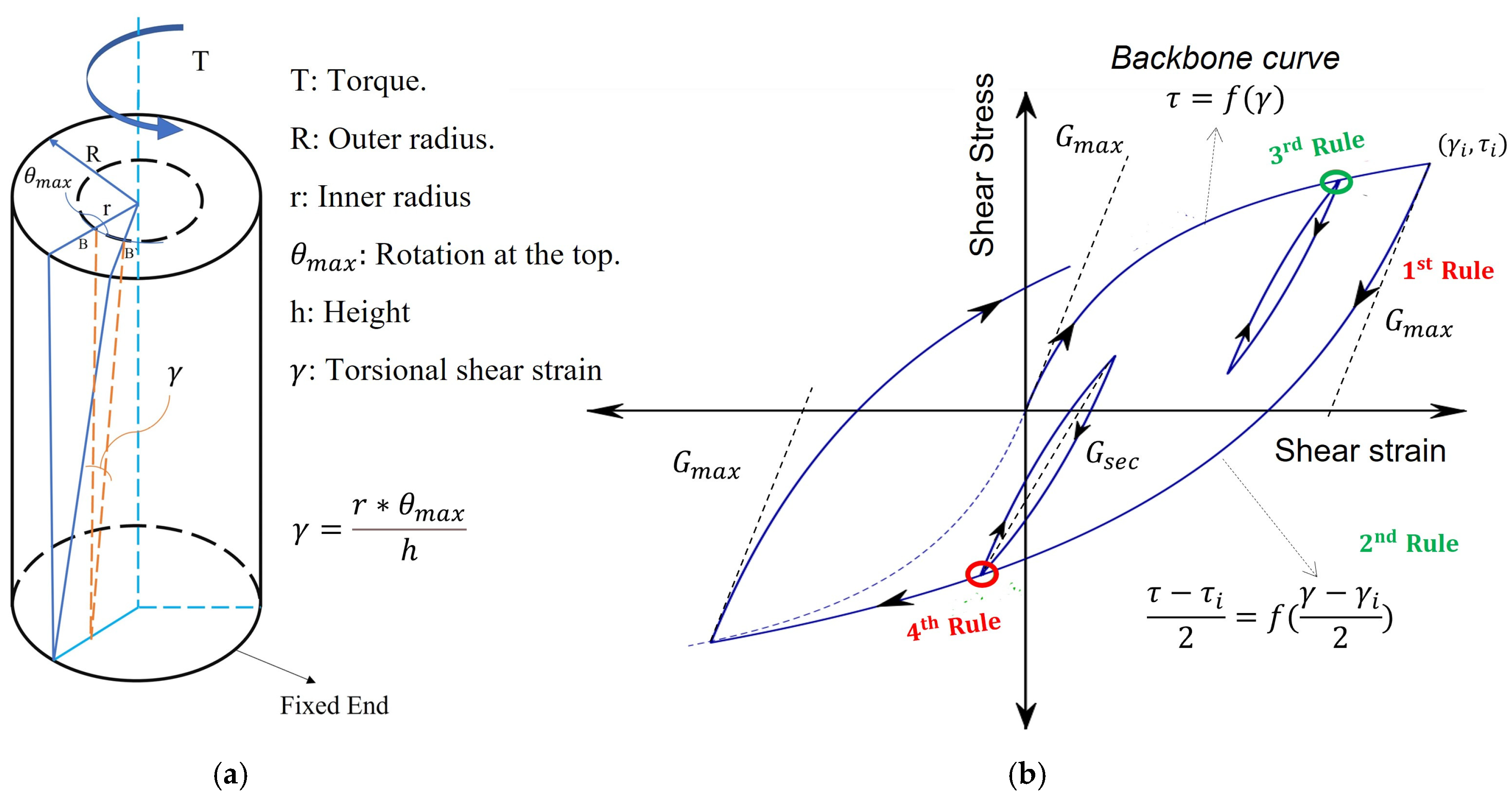
- (1)
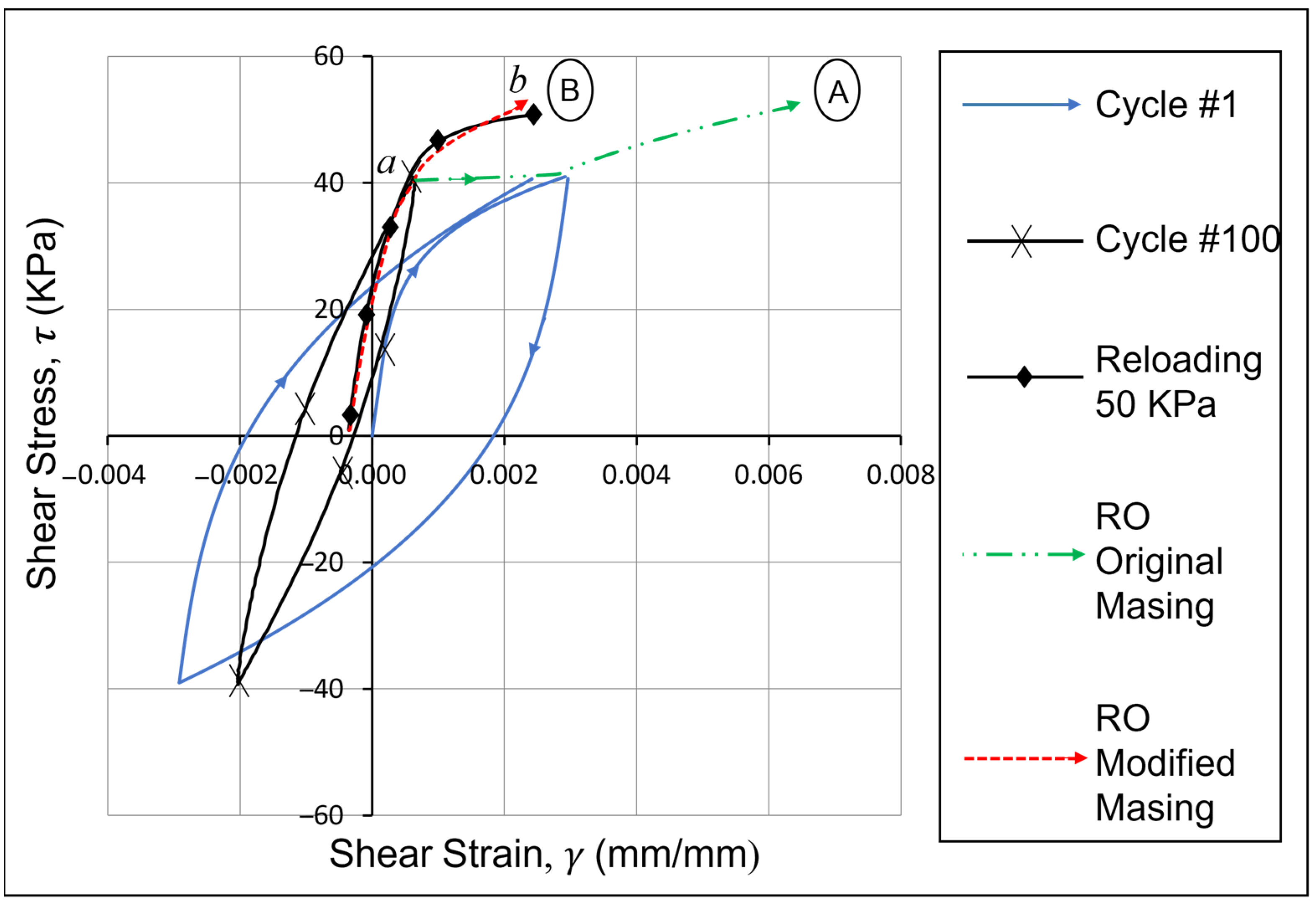
- The shear modulus in unloading/reloading is equal to the initial tangent modulus for the initial loading curve.
- (2)
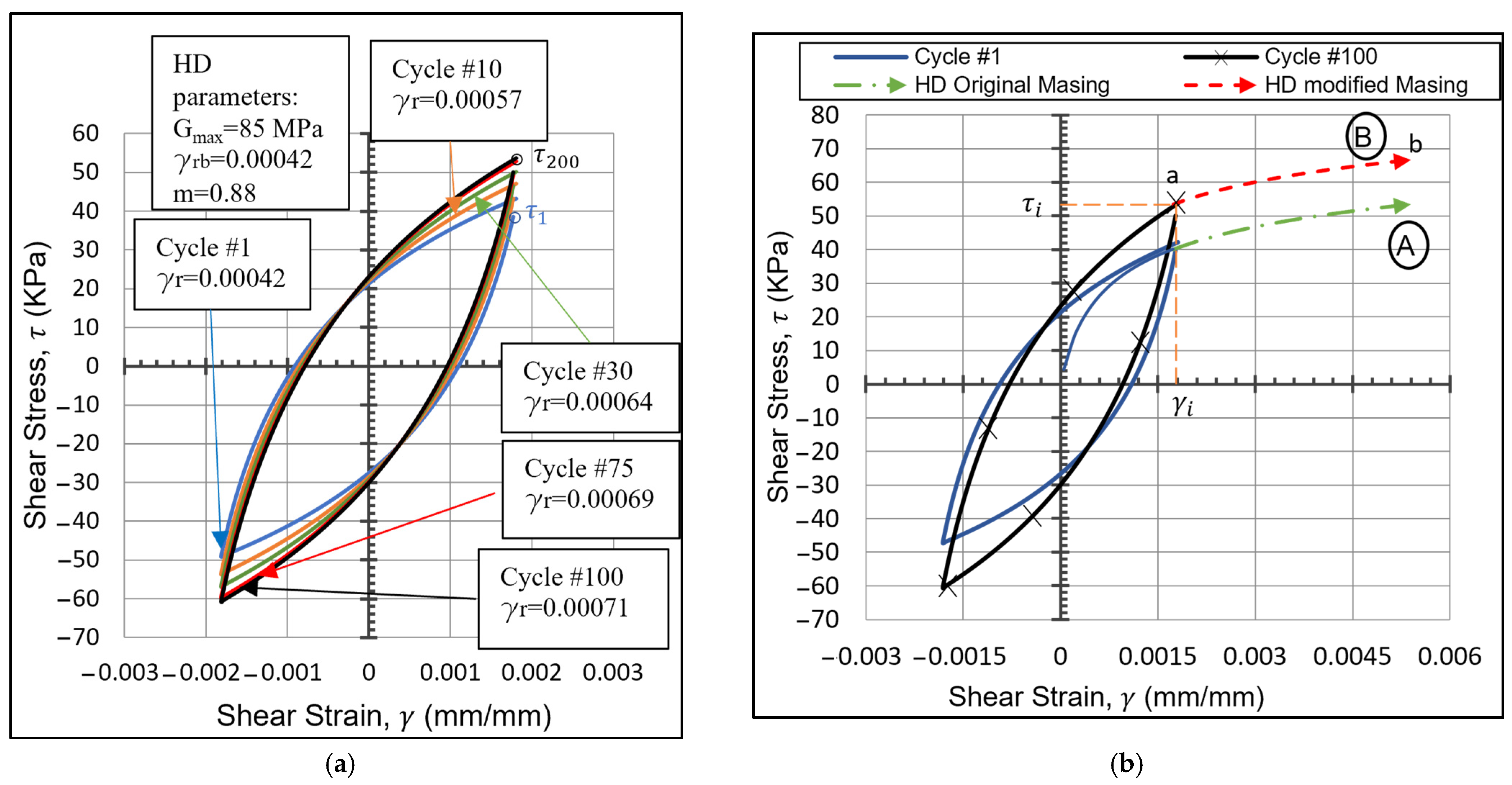
- The unloading and reloading curves duplicate the initial curve, except its scale increases by a factor of two in both directions. The variables τ and γ in the formula become and (Figure 1b).
- (3)
- The unloading and reloading curves should follow the backbone curve in the case that the previous maximum shear strain is exceeded.
- (4)
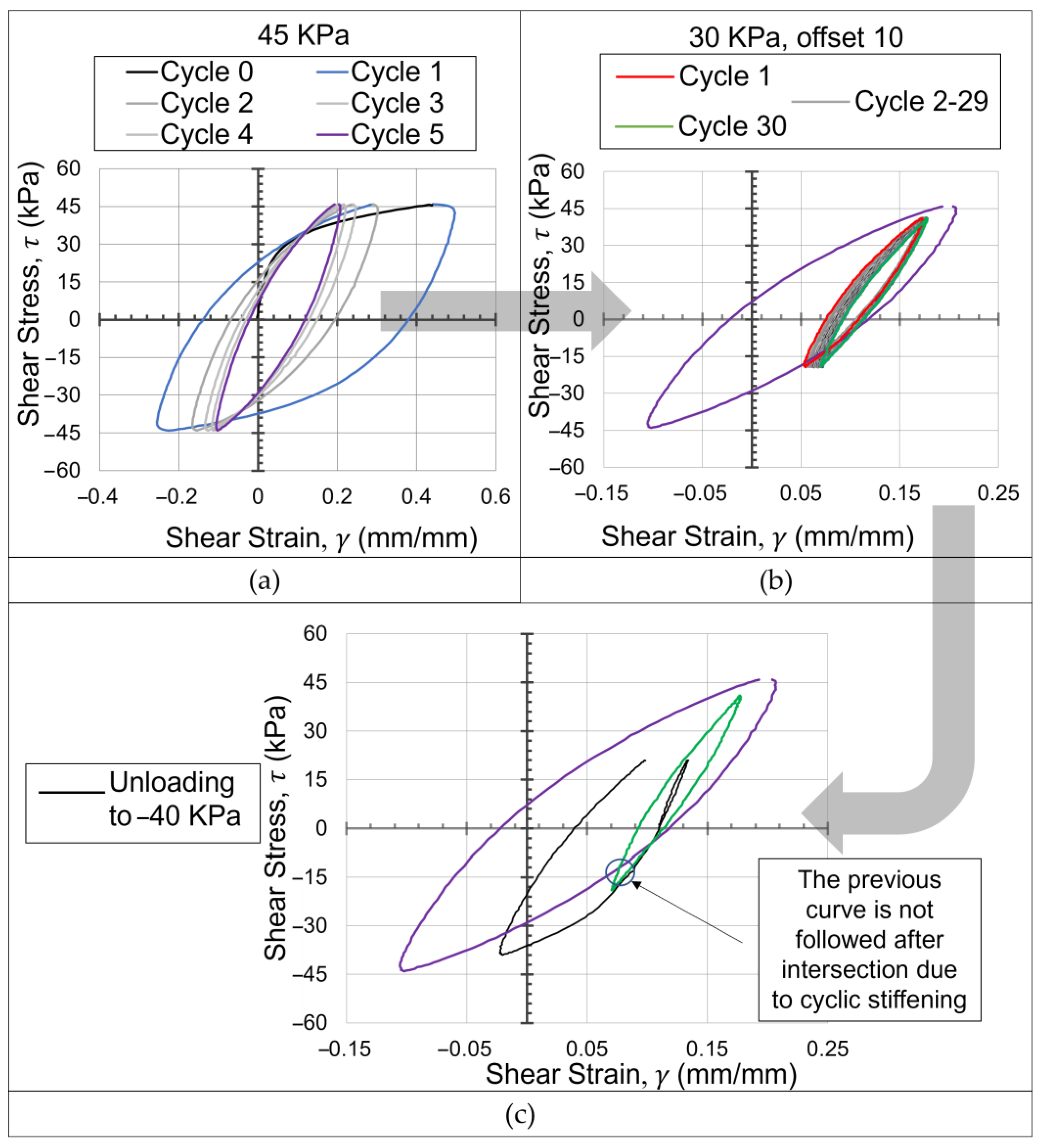
- If the current loading or unloading curve intersects a previous one, it should follow the intersected curve.
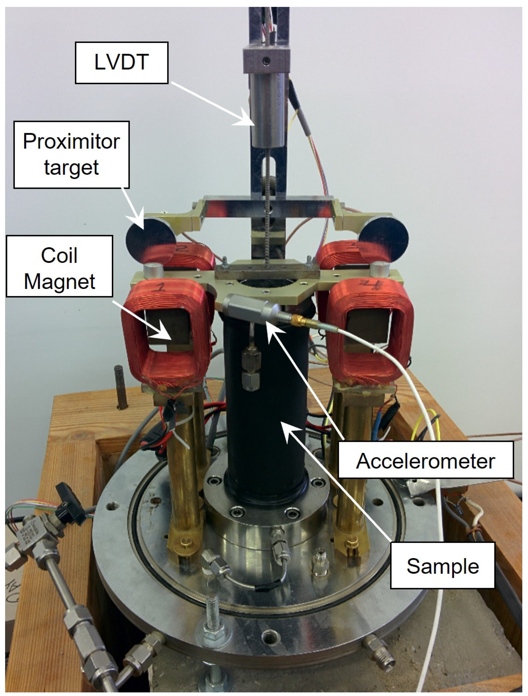
2. Testing Program
3. Original Soil Models
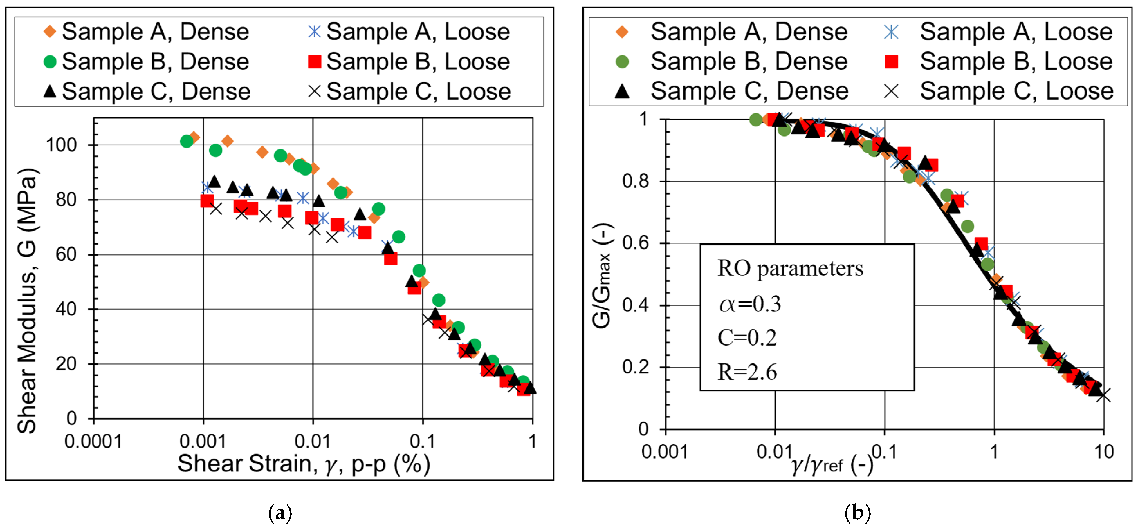
3.1. Ramberg–Osgood Model
3.2. Modified Hardin–Drnevich Model
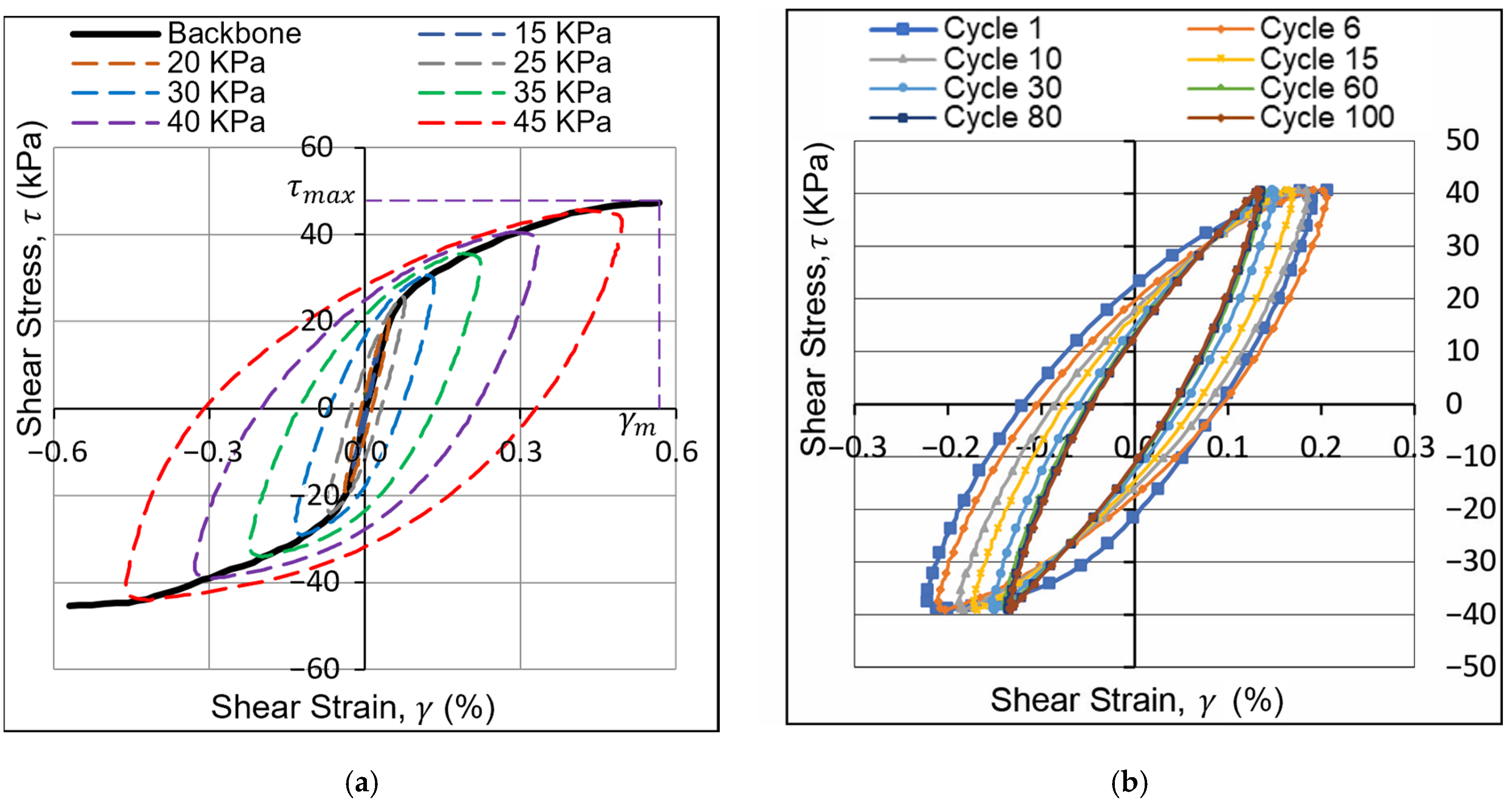
4. Results of the RC-TOSS Tests
5. Limitations of the Soil Models and Extended Masing Criteria
6. Proposed Soil Models
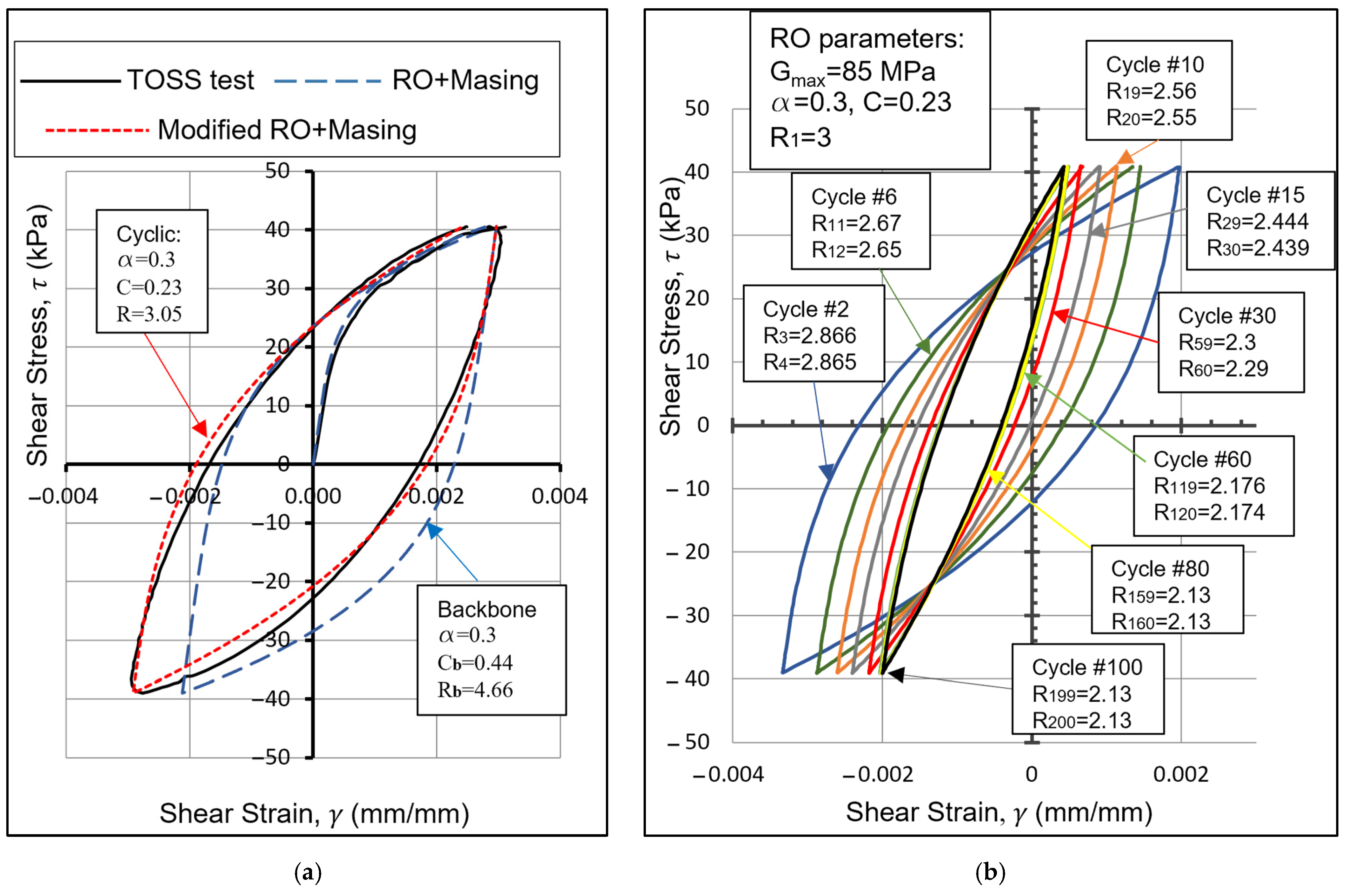
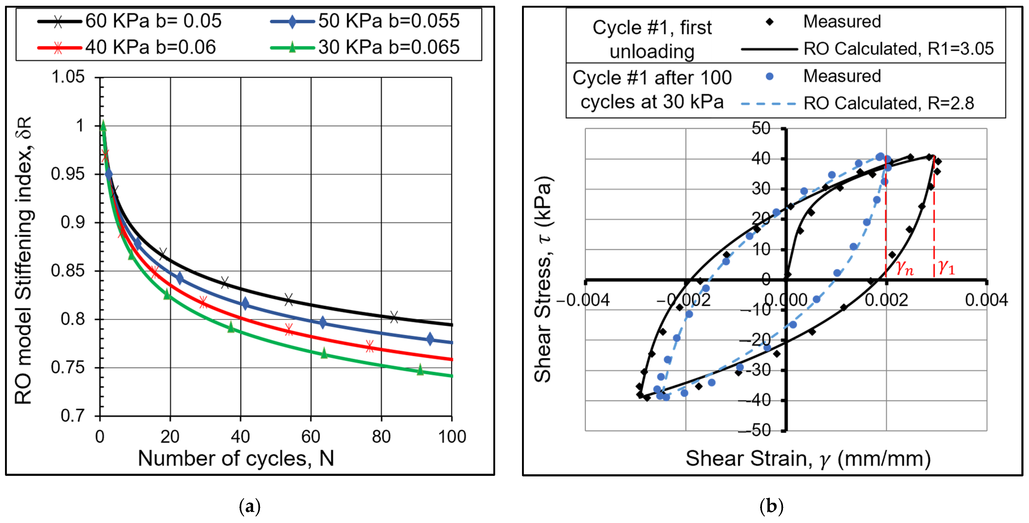
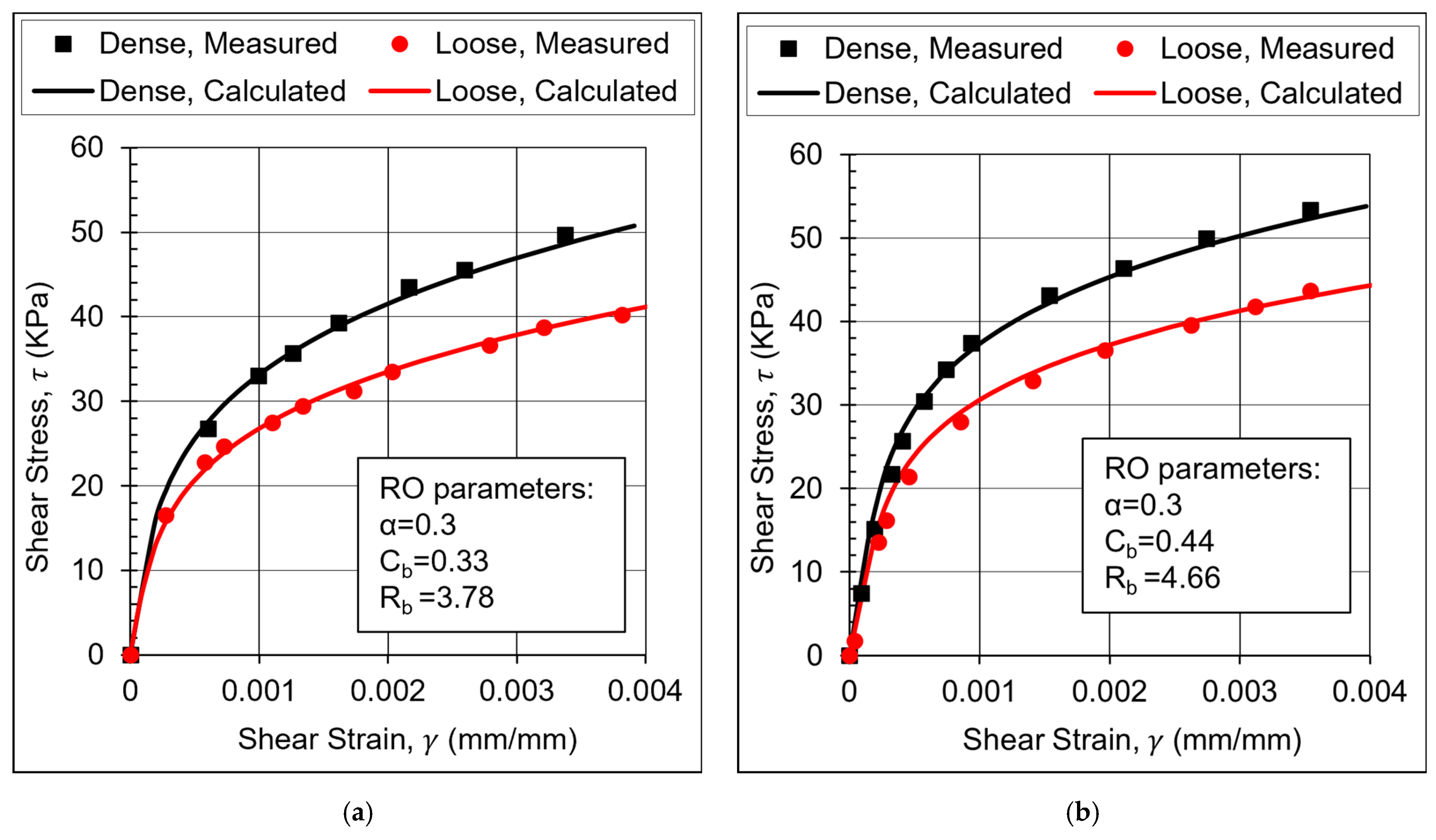
6.1. Modifications to the Ramberg–Osgood Model
6.2. Modifications to the Hardin–Drnevich Model
7. Conclusions
Author Contributions
Funding
Data Availability Statement
Conflicts of Interest
References
- Alsirawan, R.; Koch, E. Dynamic Analysis of Geosynthetic-Reinforced Pile-Supported Embankment for a High-Speed Rail. Acta Polytech. Hung. 2023, 21. [Google Scholar] [CrossRef]
- Zhao, K.; Wang, Q.; Zhuang, H.; Li, Z.; Chen, G. A fully coupled flow deformation model for seismic site response analyses of liquefiable marine sediments. Ocean Eng. 2022, 251, 111144. [Google Scholar] [CrossRef]
- Yang, H.-C.; Chou, H.-C.; Hsu, S.-Y.; Chang, W.-K. The influence of boundary conditions on nonlinear time domain site response analysis using LS-DYNA. Comput. Geotech. 2023, 159, 105477. [Google Scholar] [CrossRef]
- Wang, Y.; Liang, J.; Ba, Z. Weak nonlinear seismic response of 3D sedimentary basin using a new masing soil nonlinear model. Soil Dyn. Earthq. Eng. 2023, 171, 107982. [Google Scholar] [CrossRef]
- Ozsarac, V.; Monteiro, R.; Askan, A.; Calvi, G.M. Impact of local site effects on seismic risk assessment of reinforced concrete bridges. Soil Dyn. Earthq. Eng. 2023, 164, 107624. [Google Scholar] [CrossRef]
- Civelekler, E.; Afacan, K.B.; Okur, D.V. Effect of site specific soil characteristics on the nonlinear ground response analysis and comparison of the results with equivalent linear analysis. J. Appl. Geophys. 2024, 220, 105250. [Google Scholar] [CrossRef]
- Vucetic, M.; Vucetic, A.M.M.; Member, A.A. Cyclic threshold shear strains in soils. J. Geotech. Eng. 1994, 120, 2208–2228. [Google Scholar] [CrossRef]
- Anderson, B.A. Deformation Characteristics of Soft, High-Plastic Clays under Dynamic Loading Conditions; Chalmers University of Technology: Gothenburg, Sweden, 1979. [Google Scholar]
- Ladd, R.S. Geotechnical Laboratory Testing Program for Study and Evaluation of Liquefaction Ground Failure Using Stress and Strain Approaches: Heber Road Site, October 15, 1979 Imperial Valley Earthquake; Woodward-Clyde Consultants, Eastern Region: Wayne, NJ, USA, 1982; Volume I–III. [Google Scholar]
- Georgiannou, V.N.; Rampello, S.; Silvestri, F. Static and Dynamic Measurements of Undrained Stiffness of Natural Overconsolidated Clays. In Proceedings of the l0th European Conference on Soil Mechanics and Foundation Engineering, Florence, Italy, 26–30 May 1991; Volume 1, pp. 91–95. [Google Scholar]
- Masing, G. Internal stresses and hardening in brass. In Proceedings of the Second International Congress of Applied Mechanics, Zurich, Switzerland, 12–17 September 1926; pp. 332–335. (In German). [Google Scholar]
- Jennings, P. Earthquake Response of a Yielding Structures. J. Geotech. Eng. Div. 1965, 91, 41–68. [Google Scholar] [CrossRef]
- Constantopoulos, I.V.; Roesset, J.M.; Christian, J.T. A Comparison of Linear and Exact Nonlinear Analyses of Soil Amplification. In Proceedings of the 5th WCEE, Rome, Italy, 25–29 June 1973. [Google Scholar]
- Finn, W.D.L.; Lee, K.W.; Martin, G. An Effective Stress Model for · Liquefaction. J. Geotech-Nical Eng. Div. 1977, 103, 517–533. [Google Scholar] [CrossRef]
- Pyke, R.M. Nonlinear soil models for irregular cyclic loadings. J. Geotech. Eng. Div. 1979, 105, 715–726. [Google Scholar] [CrossRef]
- Ray, R.P.; Woods, R.D.; Ray, A.M.R.P.; Member, A.A. Modulus and damping due to uniform and variable cyclic loading. J. Geotech. Eng. 1988, 114, 861–876. [Google Scholar] [CrossRef]
- Szilvágyi, Z. Dynamic Soil Properties of Danube Sands. Ph.D. Dissertation, Széchenyi István University, Győr, Hungary, 2017. [Google Scholar]
- Valera, J.E.; Berger, E.; Kim, H.-S.; Reaugh, J.E.; Golden, R.D.; Hofmann, R. Study of Nonlinear Effects on One-Dimensional Earthquake Response; Report No. NP-865; Electric Power Research Institute: Palo Alto, CA, USA, 1978. [Google Scholar]
- Ahmad, M.; Ray, R. Comparison between Ramberg-Osgood and Hardin-Drnevich soil models in Midas GTS NX. Pollack Period. 2021, 16, 52–57. [Google Scholar] [CrossRef]
- Ray, R.P. Changes in Shear Modulus and Damping in Cohesionless Soils Due to Repeated Loading. Ph.D. Dissertation, University of Michigan, Washtenaw County, MI, USA, 1984; p. 417. [Google Scholar]
- Silver, M.L.; Seed, H.B. Volume changes in sands during cyclic loading. J. Soil Mech. Found. Div. 1971, 97, 1171–1182. [Google Scholar] [CrossRef]
- Sherif, M.A.; Ishibashi, I. Dynamic shear modulus for dry sands. J. Geotech. Eng. Div. 1976, 102, 1171–1184. [Google Scholar] [CrossRef]
- Hall, J.R.; Richart, F.E. Dissipation of Elastic Wave Energy in Granular Soils. J. Soil Mech. Found. Div. 1963, 89, 27–56. [Google Scholar] [CrossRef]
- Hardin, B.O.; Music, J. Apparatus for Vibration of Soil Specimens during the Triaxial Test, Instruments and Apparatus for Soil and Rock Mechanics; American Society for Testing and Materials: West Conshohocken, PA, USA, 1965. [Google Scholar]
- Drnevich, V.P. Effect of Strain History on the Dynamic Properties of Sand. Ph.D. Dissertation, University of Michigan, Washtenaw County, MI, USA, 1967. [Google Scholar]
- Isenhower, W.M. Torsional Simple Shear/Resonant Column Properties of San Francisco Bay Mud. Master’s Thesis, University of Texas at Austin, Austin, TX, USA, 1979. [Google Scholar]
- Ramberg, W.; Osgood, W.R. Description of Stress Strain Curves by Three Parameters; Technical Note No. 902; National Advisory Committee for Aeronautics: Washington, DC, USA, 1943. [Google Scholar]
- Streeter, V.L.; Wylie, E.B.; Richart, F.E. Soil Motion Computations by Characteristics Method. J. Geotech. Eng. Div. 1974, 100, 247–263. [Google Scholar] [CrossRef]
- Benz, T. Small Strain Stiffness of Soils and Its Numerical Consequences. Ph.D. Dissertation, Universität Stuttgart Institut für Geotechnik, Stuttgart, Germany, 2006; p. 209. [Google Scholar]
- Szilvagyi, Z.; Ray, R.P. Verification of the Ramberg-Osgood Material Model in Midas GTS NX with the Modeling of Torsional Simple Shear Tests. Period. Polytech. Civ. Eng. 2018, 62, 629–635. [Google Scholar] [CrossRef]
- Hardin, B.O.; Drnevich, V.P. Shear modulus and damping in soils: Design equations and curves. J. Soil Mech. Found. Div. 1972, 98, 667–692. [Google Scholar] [CrossRef]
- Darendeli, B. Development of a New Family of Normalized Modulus Reduction and Material Damping Curves. Ph.D. Dissertation, University of Texas at Austin, Austin, TX, USA, 2001; pp. 1–362. [Google Scholar]
- Idriss, I.M.; Dobry, R.; Singh, R.D. Nonlinear behavior of soft clays during cyclic loading. J. Geotech. Eng. Div. 1978, 104, 1427–1447. [Google Scholar] [CrossRef]
- Lin, M.L.; Chen, J.Y. Degradation Behavior of Normally Consolidated Clay under Cyclic Loading Condition; University of Missouri: St. Louis, MO, USA, 1991. [Google Scholar]
- Presti, D.C.F.L.; Cavallaro, A.; Maugeri, M.; Pallara, O.; Ionescu, F. Modelling of Hardening and Degradation Behavior of Clays and Sands During Cyclic Loading. In Proceedings of the 12th Word Conference on Earthquake Engineering, Paper n°. 1849/5/A, Auckland, New Zealand, 30 January–4 February 2000; ISBN 0-9582154-1-3. [Google Scholar]
- Lo Presti, D.C.; Lai, C.G.; Puci, I. ONDA: Computer Code for Nonlinear Seismic Response Analyses of Soil Deposits. J. Geotech. Geoenviron. Eng. 2006, 132, 223–236. [Google Scholar] [CrossRef]


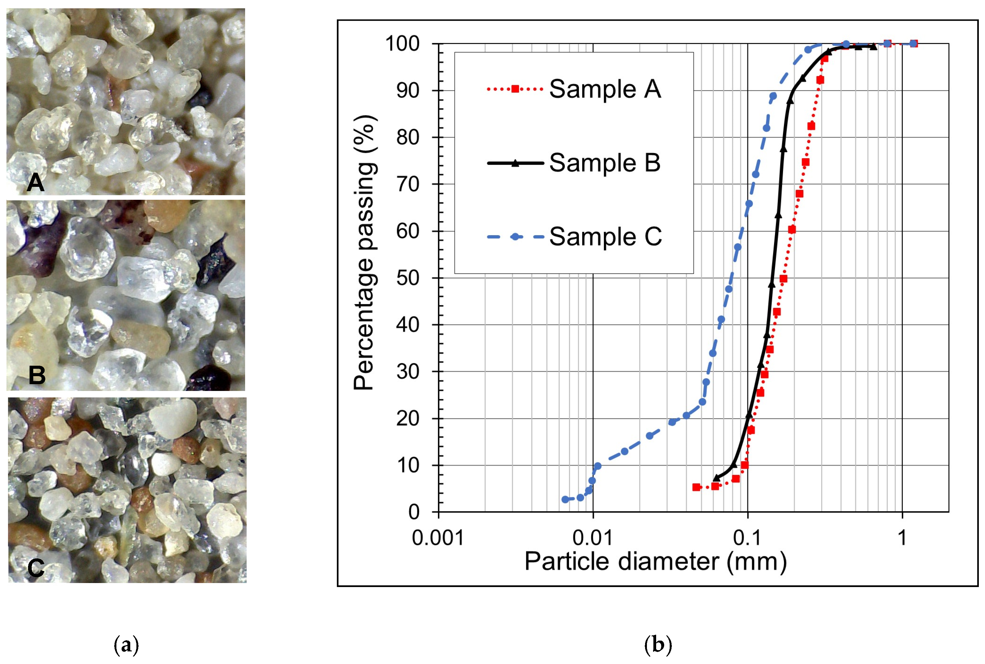
| Sample ID | Mean Particle Diameter | Eff Particle Diameter | Uniformity Coeff. | Fines Content | Max Void Ratio | Min Void Ratio | Liq. Limit for Fines | Plastic Limit for Fines | Plastic Index for Fines |
|---|---|---|---|---|---|---|---|---|---|
| d50 (mm) | d10 (mm) | Cu (-) | FC (%) | emax (-) | emin (-) | wl (%) | wp (%) | Ip (%) | |
| A | 0.211 | 0.109 | 2.06 | 7.56 | 0.81 | 0.52 | - | - | |
| B | 0.243 | 0.130 | 2.18 | 5.69 | 0.79 | 0.516 | - | - | |
| C | 0.107 | 0.013 | 9.85 | 21.11 | 0.9 | 0.524 | 30.4 | 19.7 | 10.7 |
| Test Number | Sample ID | Confining Stress | Void Ratio | Relative Density | Angle of Friction | Test Type |
|---|---|---|---|---|---|---|
| # | P′ (kPa) | e (-) | Dr (-) | (o) | ||
| 1–2 | A | 97 | 0.77 | 0.14 | 31 | Cyclic RC-TOSS |
| 3–4 | A | 97 | 0.58 | 0.79 | 40 | Cyclic RC-TOSS |
| 5–6 | B | 96.5 | 0.76 | 0.11 | 35 | Cyclic RC-TOSS |
| 7–8 | B | 96.5 | 0.57 | 0.80 | 43 | Cyclic RC-TOSS |
| 9–10 | C | 97 | 0.85 | 0.13 | 31 | Cyclic RC-TOSS |
| 11–12 | C | 97 | 0.62 | 0.74 | 40 | Cyclic RC-TOSS |
| 13 | A | 97 | 0.58 | 0.79 | 40 | TOSS, effect of stress offset |
| 14 | B | 97 | 0.58 | 0.77 | 43 | TOSS, effect of stress offset |
| Test Number | Sample ID | Uniformity Coeff. | Fines Content | Void Ratio | Maximum Shear Modulus | Maximum Shear Stress | Cb | Rb | |
|---|---|---|---|---|---|---|---|---|---|
| # | Cu (-) | FC (%) | e (-) | Gmax (MPa) | (kPa) | (-) | (-) | (-) | |
| 1 | A | 2.06 | 7.56 | 0.77 | 85 | 40 | 0.3 | 0.33 | 3.78 |
| 3 | A | 2.06 | 7.56 | 0.58 | 103.4 | 50 | 0.3 | 0.33 | 3.78 |
| 5 | B | 2.18 | 5.69 | 0.76 | 79.6 | 44 | 0.3 | 0.44 | 4.66 |
| 7 | B | 2.18 | 5.69 | 0.57 | 100 | 53 | 0.3 | 0.44 | 4.66 |
| 9 | C | 9.85 | 21.11 | 0.85 | 76 | 40 | 0.3 | 0.29 | 3.35 |
| 11 | C | 9.85 | 21.11 | 0.62 | 87 | 50 | 0.3 | 0.29 | 3.35 |
|
Test Number | Sample ID | Max Shear Modulus |
Max Shear Stress | C | R1 * | b ** | k *** | |
|---|---|---|---|---|---|---|---|---|
| # | Gmax (MPa) | (kPa) | (-) | (-) | (-) | (-) | ||
| 1 | A | 85 | 40 | 0.3 | 0.23 | 0.06 | ||
| 2 | A | 103.4 | 50 | 0.3 | 0.23 | 0.06 | ||
| 3 | B | 79.6 | 44 | 0.3 | 0.23 | 0.055 | ||
| 4 | B | 100 | 53 | 0.3 | 0.23 | 0.04 | ||
| 5 | C | 76 | 40 | 0.3 | 0.15 | kPa | ||
| 6 | C | 87 | 50 | 0.3 | 0.15 |
| Test Number | Sample ID | Maximum Shear Modulus | m | f * | s ** | ||
|---|---|---|---|---|---|---|---|
| # | Gmax (MPa) | (-) | (-) | (-) | (-) | (-) | |
| 1 | A | 85 | 0.00042 | 0.88 | 0.00042 | 0.1 | |
| 2 | A | 103.4 | 0.00042 | 0.88 | 0.00042 | 0.09 | |
| 3 | B | 79.6 | 0.0005 | 0.88 | 0.00047 | 0.085 | |
| 4 | B | 100 | 0.0005 | 0.88 | 0.00047 | 0.063 | |
| 5 | C | 76 | 0.00053 | 0.88 | 0.0005 | 0.095 | |
| 6 | C | 87 | 0.00053 | 0.88 | 0.0005 | 0.11 |
Disclaimer/Publisher’s Note: The statements, opinions and data contained in all publications are solely those of the individual author(s) and contributor(s) and not of MDPI and/or the editor(s). MDPI and/or the editor(s) disclaim responsibility for any injury to people or property resulting from any ideas, methods, instructions or products referred to in the content. |
© 2024 by the authors. Licensee MDPI, Basel, Switzerland. This article is an open access article distributed under the terms and conditions of the Creative Commons Attribution (CC BY) license (https://creativecommons.org/licenses/by/4.0/).
Share and Cite
Ahmad, M.; Ray, R. Modeling the Stiffening Behavior of Sand Subjected to Dynamic Loading. Geosciences 2024, 14, 26. https://doi.org/10.3390/geosciences14010026
Ahmad M, Ray R. Modeling the Stiffening Behavior of Sand Subjected to Dynamic Loading. Geosciences. 2024; 14(1):26. https://doi.org/10.3390/geosciences14010026
Chicago/Turabian StyleAhmad, Majd, and Richard Ray. 2024. "Modeling the Stiffening Behavior of Sand Subjected to Dynamic Loading" Geosciences 14, no. 1: 26. https://doi.org/10.3390/geosciences14010026
APA StyleAhmad, M., & Ray, R. (2024). Modeling the Stiffening Behavior of Sand Subjected to Dynamic Loading. Geosciences, 14(1), 26. https://doi.org/10.3390/geosciences14010026