Deep Neural Networks for the Estimation of Masonry Structures Failures under Rockfalls

Abstract

Although the principal aim of the rockfall management is to prevent rock boulders from reaching the buildings instead of the buildings resisting the boulder impacts, there usually exists a residual risk that has to be assessed, even when structural protection measurements are taken. The evaluation of the expected damage of buildings due to rockfalls using empirical data from past events is not always possible, as transferring and applying damage observations from one area to another can be unrealistic. In order to simulate potential rockfall scenarios and their damage on buildings, numerical methods can be an alternative. However due to their increased requirements in expertise and computational costs, their integration into the risk analysis is limited, and simpler tools to assess the rockfall vulnerability of buildings are needed. This paper focuses on the application of artificial intelligence AI methods for providing the expected damage of masonry walls which are subjected to rockfall impacts. First, a damage database with 672 datasets was created numerically using the particle finite element method and the finite element method. The input variables are the rock volume (VR), the rock velocity (RV), the masonry wall (t) and the masonry tensile strength ${\mathrm{f}}_{\mathrm{m}}$. The output variable is a damage index (DI) equal to the percentage of the damaged wall area. Different AI algorithms were investigated and the ANN LM 4-21-1 model was selected to optimally assess the expected wall damage. The optimum model is provided here (a) as an analytical equation and (b) in the form of contour graphs, mapping the DI value. Known the VR and the RV, the DI can be directly used as an input for the vulnerability of masonry walls into the quantitative rockfall risk assessment equation.

1. Introduction

The damage of buildings caused by rockfalls can be devastating. The expansion of urban areas toward rocky slopes, on the one hand, and the temperature and rainfall extremes which have been observed in the past decades and have been associated with climate change, on the other, have been intensifying the disastrous phenomena, with direct (physical) and indirect (social, economic) impacts. Although the rockfall impacts are not as extensive as the earthquake impacts, their sum is substantial.

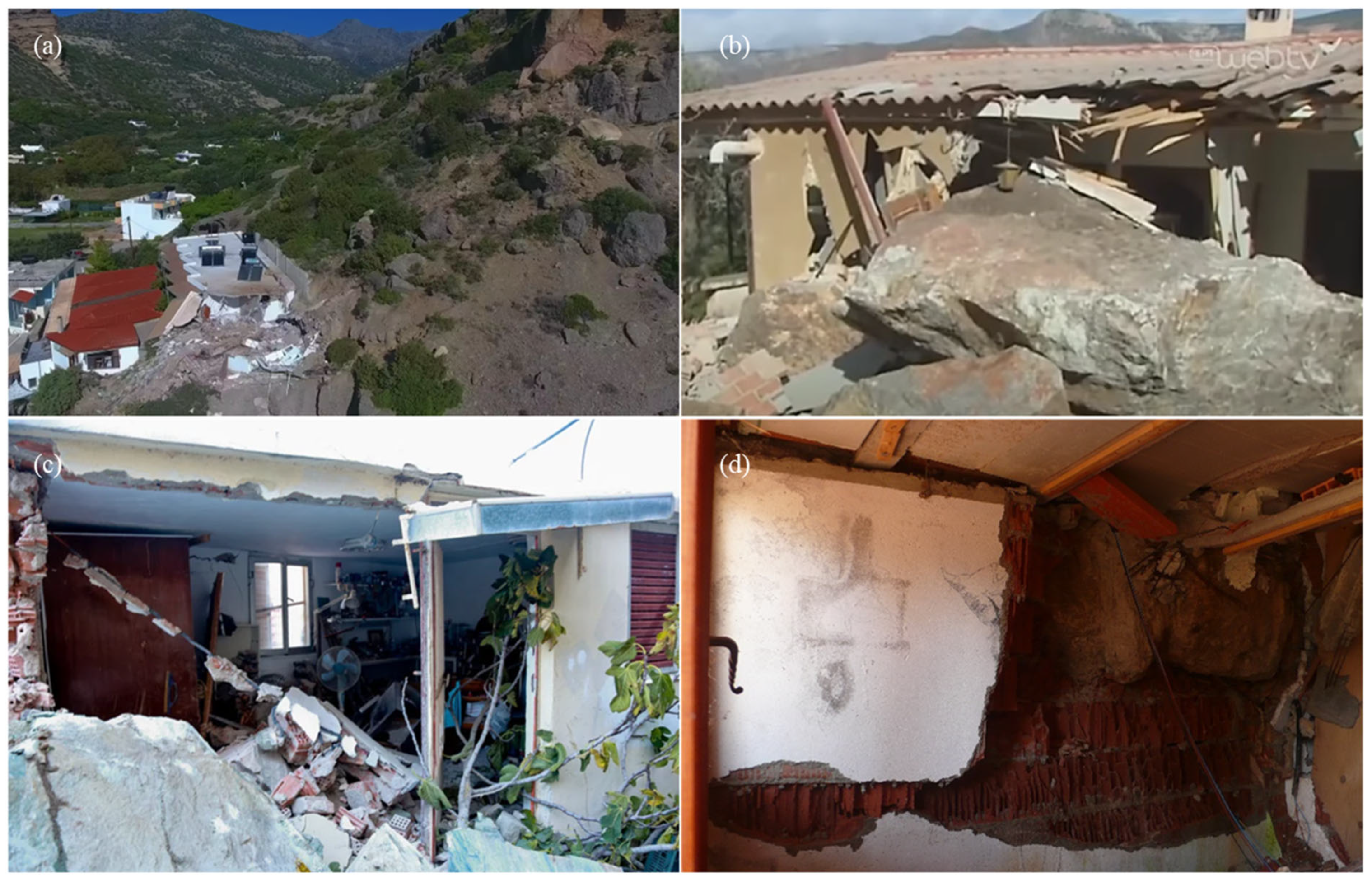
Figure 1 shows characteristic examples of building damage caused by rockfalls. In Greece, in 2022, a rockfall in Crete killed a person hosted in a touristic apartment. In 2018, on the island of Mytilene, a residential area was affected by rockfalls and 14 houses were evacuated. The wall of a house was destroyed by a rock block of about 15 m³, in Alyki, Viotia, in 2019. Worldwide, several urbanisms have been damaged by rockfalls, amongst others during the 2015 Gorkha earthquake in Nepal and the 2011 Christchurch earthquake in New Zealand. Residences in mountainous villages such as the Clua in the Pyrenees, Spain, are threatened by rockfalls, while touristic infrastructure is affected frequently, as in the case of a hotel in Bolzano, in the Alps, which was hit by a rockslide in 2021. Further examples in Central Italy are presented in [1].

The rockfall quantitative risk assessment is a powerful tool for expressing the expected loss in objective terms, which are usually financial (e.g., €/year). The expected damage for buildings which are exposed to rock block impacts during rockfalls is required as an input for the rockfall quantitative risk assessment [2]. Although there exist sophisticated and detailed methodologies for the assessment of the rockfall hazard and risk, the rockfall structural vulnerability is still scarcely deepened [3]. The existing research work in this field is limited compared to the work on the protection measures that aim at the stabilization, interception, or catchment of rock blocks. This is ought to the fact that the rockfall risk reduction is far more effective when aiming at the installation of protection measures, rather than at the reinforcement of buildings against rockfalls. Accordingly, the relatively few studies on the rockfall damage of buildings focus on providing the expected damage to be used for the QRA instead of discussing strengthening measures.

The approaches for assessing the damage of buildings due to rockfalls include empirical methods, which are based on the observation of damage from past events [4,5]. An example of an empirical database has been presented by [6], who registered the rockfall damage of buildings at the Christchurch earthquake and mapped it using a terrestrial laser scanner (TLS). A good correlation was indicated between the damage extent, in terms of affected area inside the building, and the rock block kinetic energy. Empirical methods can associate the damage with the rock motion properties (size and impact velocity). The advantage of empirical methods is that they can take into consideration the existence of non-structural details as for example the presence of openings and protective elements around the building. However, they, usually, do not differentiate between building typologies and characteristics.

The use of computational methods to model the behavior of buildings that are affected by fast moving landslides is less common, although it has been well established for rockfall protection measures [7]. A numerical methodology for the calculation of fragility curves for reinforced concrete buildings in areas affected by earthquake-induced landslides has been developed by [8]. This methodology is applicable to a variety of soil types, slopes, and buildings. Fragility curves for reinforced concrete buildings subjected to differential settlements caused by landslides have been calculated at [9], based on the statistical processing of the damage that has been obtained by structural numerical analysis. More recently, the Material Point Method was proposed by the authors in [10] to investigate the landslide–structure interaction, using a coupled approach for simulating the fast propagation of a saturated soil and the stress–strain response of a masonry structural element.

In particular for rockfalls, analytical and numerical methods have been investigated for the assessment of the damage of reinforced concrete and masonry buildings by [11,12]. A methodology was presented at [13] for the assessment of damage of masonry structures due to rock block impacts. The methodology considers the wall characteristics (wall width and material properties) and the rock block properties (velocity and volume). The back analysis of three rockfalls causing damage to masonry walls was made. The damage was expressed in terms of a damage index DI that is equal to the percentage of the damaged surface divided by the total surface of the wall.

Although analytical methods provide flexibility in modelling different scenarios of structural element typologies and rock properties, they are difficult to be applied by non-experts, and their direct integration into the rockfall risk assessment is not effective, in terms of cost and time. The application of damage predictive mathematical models that use a regression equation, based on the observed damage from real events, as proposed by [5], could overcome this issue.

The value of the aforementioned masonry structure damage index DI has a strong nonlinear nature regarding its correlation with the mechanical and geometrical characteristics of the masonry as well as with the volume and speed of the impacting rock blocks. This makes difficult the prediction of masonry wall failure using deterministic classical computational techniques, such as the least square method and regression analysis-based approaches.

For the simulation of this kind of highly nonlinear phenomena, soft computing techniques such as artificial neural networks (ANN) have been proposed, during the last three decades, with many applications to medicine [14,15,16,17,18,19]. These applications have been growing rapidly in engineering over the last two decades [20,21,22,23,24,25,26,27,28,29,30,31,32]. The main disadvantage of these techniques has been reported to be that their function is a black box, thus despite the plethora of relevant publications, the results are not transferable. To overcome this limitation, during the past decade, particular emphasis has been put on the formulation of analytical equations that describe the architecture of the structure of ANN’s. Many of the relevant publications contain as Supplementary Materials, graphical user interfaces (GUI) to verify their reliability and to permit their use by other researchers [33,34,35,36].

In this work, a big analytical database has been developed for the training of deep neural networks, aiming at the development of a robust and reliable forecasting mathematical model for the estimation of the rockfall damage of masonry structures. The analytical database was developed using numerical methods in order to calculate the aforementioned quantitative DI. Furthermore, a closed-form equation (analytical formula) has been derived, based on the optimal ANN model.

The paper is organized in seven sections. In Section 2, the research significance of this work for rockfall risk assessment studies is discussed. Section 3 focuses on the numerical analysis that has been made for the creation of the damage database. Section 4 presents the materials and methods that were used for the development of the forecasting mathematical model for the damage index. Section 5 provides a closed-form equation for the estimation of the damage index and its mapping. In Section 6, the limitations of the proposed model are presented and in Section 7, some concluding remarks.

2. Research Significance

Load-bearing masonry structures are common in mountainous areas where rockfall events occur frequently. The methodology which is presented here is focused on the assessment of the damage of walls due to rockfall impacts. Risk assessment for rockfalls can be expressed quantitatively using the following equation, adapted from [37], which should be summed up for all the expected rockfall magnitudes and intensities:

$$\mathrm{R}=\mathrm{P}\left(\mathrm{L}\right)\times \mathrm{P}\left(\mathrm{T}:\mathrm{L}\right)\times \mathrm{P}\left(\mathrm{S}:\mathrm{T}\right)\times \mathrm{V}\left(\mathrm{E}:\mathrm{S}\right)\times \mathrm{C}$$

(1)

where:

$\mathrm{R}$ is the risk in terms of expected annual loss;

$\mathrm{P}\left(\mathrm{L}\right)$ is the annual frequency of the rockfall events of a given magnitude;

$\mathrm{P}\left(\mathrm{T}:\mathrm{L}\right)$ is the probability of a rockfall reaching the element at risk with a given intensity;

$\mathrm{P}\left(\mathrm{S}:\mathrm{T}\right)$ is the temporal spatial probability of the element at risk;

$\mathrm{V}\left(\mathrm{E}:\mathrm{S}\right)$ is the vulnerability of the element at risk for a rockfall event of a given magnitude and intensity;

$\mathrm{C}$ is the cost of the element at risk.

For buildings, the vulnerability expresses the expected degree of loss, on a scale of 0 (no loss) to 1 (total loss).

Taking into consideration the limitations of the empirical and analytical methods for the damage assessment that were explained in Section 1, risk assessment practitioners require simple-to-use tools, in order to obtain vulnerability values for the application of Equation (1). To fill this gap, the goal of this work was to develop a closed-form equation (analytical formula) for the vulnerability that takes into account the complexities of masonry response, based on an analytically derived wall damage database and an ANN model.

The work presented here takes into consideration only the damage of the wall elements. The proposed damage index DI to be used for the vulnerability value, as it will be explained in detail in the following sections, is given by Equation (2).

DI = Damaged wall area/Total wall area

(2)

This DI does not provide direct information for the loss of the overall stability of the building, nor for the propagation of the block into the building, although these two are key factors for the extent of structural and non-structural damage that will determine the repair cost of the building, as well as the exposure of the people within it. A thorough investigation of these has been out of the scope of the present work. Nevertheless, it is expected that the larger the DI, the larger the affected area, because of the higher kinetic energy of the rock. Accordingly, the exposure of people inside the building will be increased. The overall stability of the structure depends on the specific setting of the building. Despite of structures made of masonry walls being statically indeterminate, high energy rock impacts may lead to overall building damage and collapse. However, in order to incorporate this into the vulnerability value, a more precise analysis for a specific building setting would be required.

3. Rockfall Impact Force and Wall Damage Assessment

As aforementioned, given the difficulties for obtaining a large and comprehensive wall damage database from historical events, a numerical methodology was preferred for the database creation. The methodology, which was introduced by [13] consists in the coupling of two separate numerical processes: (1) first, the rockfall actions which are transmitted from the rock block to the wall during the block-wall interaction are calculated for a selected range of rock block sizes and wall characteristics, using a numerical model, and then (2) the predicted rockfall action contact forces are applied as an external load to the wall in order to calculate the DI. For the completeness of the paper, the processes are briefly described.

3.1. Rockfall Impact Forces

Besides the velocity and kinetic energy of the rock boulder, the transmission of energy from the impacting rock to the wall depends on: the geometry of the impacting bodies, the relative stiffness, the absorbed local energy in the contact zone (damage produced), the loading time-evolution and the impact area [13]. The shape of the boulder also affects the motion properties of the rock, before and after the impact, and its potential bouncing. Given the large amount of the uncertainty that is involved, on top of the characteristic inhomogeneity of masonry structures, the numerical analysis of the impacts aims at providing an indication of the expected impact force rather than a precise value of it.

The particle finite element method (PFEM) coupled with the contact domain method (CDM) was used for being appropriate to capture the impact characteristics of a rock boulder on a masonry wall, as described in [13]. The PFEM is founded on the Lagrangian description of particles and motion, and it combines a meshless definition of the continuum containing a cloud of particles with standard mesh-based finite element techniques. The initial developments of the particle finite element method (PFEM) took place in the field of fluid mechanics [38,39] because of the PFEM capability of tracking and modelling free surfaces. Later on, the particle finite element (PFEM) was applied to a variety of simulation problems and to solid mechanics, with the first applications to problems involving large strains and rotations, multiple body contacts, and creation of new surfaces (riveting, powder filling, ground excavation and machining) [40].

Using the PFEM for the modelling of large deformations and the contact domain method (CDM), the transmission of the forces to the wall can be simulated properly. According to this method [41] there is no contact stiffness parameter (or penalty parameter). The method uses a Lagrange Multiplier approach to impose the contact constraint, which involves a remeshing strategy, for the geometrical contact detection. We apply this strategy in the particle finite element method to detect the contact area and the active contact set. The constraints are imposed directly at the balance equations.

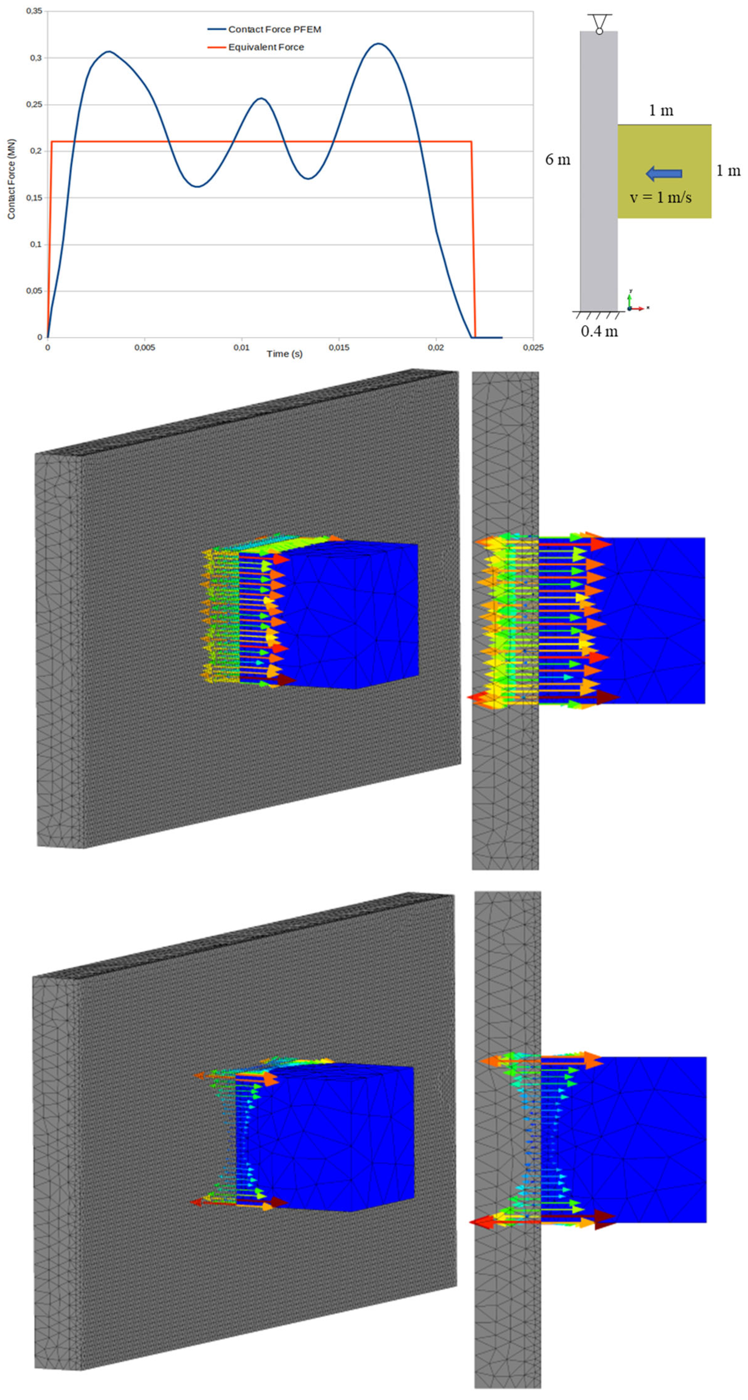
Different models have been used for the solution of the contact problem: two-dimensional (plane-strain), axisymmetric, and three-dimensional. We studied the results from the three different models, to conclude that for the given wall-block system the transmitted forces of the three formulations are of the same order of magnitude. A two-dimensional approach was preferred for reasons of time efficiency and for reducing the computational cost. The model is shown in Figure 2.

As the transmitted forces vary with time, the envelope of the maximum contact forces and the stress distribution in the direction of the movement are extracted. The following assumptions were made for the simplification of the problem.

Both masonry and rock were considered homogenous, elastic, and deformable bodies, with properties described by the modulus of elasticity, E, the Poisson ratio, v, and the density. The variation of the stiffness of the rock representing different rock lithologies was not considered for the presented analysis and it has not been included in the variables. A fixed value of the Young’s modulus equal to E = 10 GPa has been assumed, which corresponds to a unique rock type. This value tends to the lower end of the Young’s moduli encountered for sedimentary rocks.

An elastic contact was assumed, according to which the energy is not damped. The modelling of the damage around the contact area due to the rock-block contact is made in a second computational stage in order to be able to define study cases with bounded complexity. The numerical modelling of the damage and the fracture combined with the rock impact is a very interesting problem but it remains very difficult to characterize. So, in this first stage, for the calculation of the contact forces, the assumption of no damage during the rock-wall contact was made. It is expected that in the case of damage, part or the total of the block energy will be absorbed so that the block does not rebound. Parametric simulations considering continuous damage with small rock mass and impact velocity indicated that the total contact energy is preserved, and that the resulting contact forces are of the same order of magnitude as in the elastic case, however the rebound is damped. Thus, it is considered that the assumption of no damage is slightly more conservative and it is easier to be reproduced by other researchers.

A cubic block shape was assumed, with edge length calculated to provide each time the total boulder volume. Besides cubic, different shapes of rock blocks may be assumed (spherical, polyhedric…), resulting in differences in the estimated contact area. The assumption of a cube simplifies the extraction of the geometry of the contact area, being the same with the cube edge. It is highlighted that assuming a cubic rock shape and a full rock-wall contact is not conservative concerning the stresses developed on the wall, considering the much larger contact area than in the case of a spherical rock. Furthermore, the rotational velocity of the spherical rock could contribute to the damage of the wall, which is a scenario that has not been investigated in this work. The casuistry of possible rock shapes, trajectories, and contact zones is enormous and must be generalized in some way. The selection of the cubic block was made in this work in order to simplify the calculations related to the force application area on the wall.

With respect to the last point, a further assumption was made for the determination of the impact stress distribution area. For cubic blocks, the application area is initially expected to be the same as the cube edge, given that when the impact starts, the two bodies are in full contact. However, the analysis indicates that for flexible walls, right after the first contact, due to flexure around the horizontal and vertical axis passing from the center of the wall, the block forces get concentrated near the cube edge boundaries and they are calculated by the PFEM accordingly. This provides different evolutions of the interaction force, changing the magnitude of the contact forces with time. In higher speed contacts, some oscillations are also present, which is a known numerical instability resulting from numerical time integration when modelling impact problems. To overcome these issues an equivalent force was calculated, based on the balance of the produced impulses, as given by Equation (3). We determined the contact duration as the total time during which there is partial or total contact between the two bodies, considering the presence or absence of contact forces.

$$\mathrm{J}=\int \mathrm{Fdt}$$

(3)

where

$\mathrm{J}$: impulse

$\mathrm{F}$: transmitted force to the wall during the total contact time t.

For the development of the damage database, which is presented in detail in Section 4, walls of 3 m height with 6 m length, with width varying between 0.40 m and 1 m, and blocks of 1 m³ to 20 m³, with velocities ranging from 1 m/s to 30 m/s were considered. The homogenized material mechanical properties are calculated according to Eurocode 6 and specifically § 3.6.2.3 for the compressive strength and § 3.6.3 for the wall tensile strength [42], for stone units and general-purpose mortar.

An illustration of the contact forces calculation is given in Figure 2. In this example, the rock boulder is a quadrilateral of 1 × 1 m² with an initial velocity of 1 m/s. The wall was fixed at it base. The wall has been considered fixed at its base to simulate the foundation. Rotational degrees of freedom were attributed to the top nodes. The main reason for choosing the hinge at the top was to simulate rotations due to out of plane loading. The parametric analyses indicated the minimum and maximum values for the equivalent forces (

Table 1. Equivalent theoretical forces and tension transmitted to the wall from the block impact, for the four extreme scenarios of the parametric analysis.

Rock Volume (m3)	Rock Velocity (m/s)	Wall Thickness (m)	Numerical Force (MN)	Equivalent Theoretical Force (MN)	Application Area (m2)	Equivalent Tension (MPa)
1	1	0.4	0.210	0.227	1 × 1	0.227
1	1	1.0	0.307	0.352	1 × 1	0.352
20	30	0.4	106.870	112.880	2.7 × 2.7	15.473
20	30	1.0	153.010	164.830	2.7 × 2.7	22.610

).

3.2. Wall Damage

Finite element analysis has been widely used for the numerical calculation of stress and strain state of masonry walls [43,44,45]. Besides permanent and functional loads, there is a wide literature on the seismic behavior of masonry walls, however there are less works on the impact behavior of wall structures. The stress–strain response of reinforced masonry structures due to debris flow impact has been studied by [46]. Wall displacements due to boulder impacts were studied in [47], assuming different wall thicknesses and masonry mechanical characteristics. To the knowledge of the authors, there are scarce studies that quantify the expected damage considering a variety of boulder kinematics.

To fill this gap, the methodology that has been described in detail at [13] was used here. Using the software SAP2000, three-dimensional finite element models of the afore-mentioned walls were developed. For the stress analysis, the same constitutive laws were applied for the wall, as described in Section 3.1.

The stress results for the top and bottom faces of the shell elements were processed using the FAILURE software developed by [48]. The software is compatible with the stress output from the finite element analysis and applies a modified Von-Mises criterion which is specifically adapted for masonry structures.

The modified Von-Mises criterion (Figure 3) consists in a failure curve which is formed by four surfaces S₁, S₂, S₃, and S₄ (section on the horizontal plane of zero shear stress). Each surface represents a certain biaxial stress state: S₁ represents compression in parallel to both principal axes, S₂ tension in parallel to one principal axis and compression in parallel to the other, S₃ tension in parallel to both principal axes and S₄ vice versa to S₃. Failure occurs for a point on the circumference or outside the closed curve area. The curves are given by Equations (4)–(7).

The surfaces which are illustrated in Figure 3 are given by:

$${\mathrm{S}}_1={\mathsf{\sigma }}_{\mathrm{xx}}^2+{\mathsf{\sigma }}_{\mathrm{yy}}^2-{\mathsf{\sigma }}_{\mathrm{xx}}{\mathsf{\sigma }}_{\mathrm{yy}}+3{\mathsf{\tau }}^2-{\mathrm{f}}_{\mathrm{wc}}^2=0,{\mathrm{for}\mathsf{\sigma }}_{\mathrm{xx}}{\mathrm{and}\mathsf{\sigma }}_{\mathrm{yy}}\le 0$$

(4)

$${\mathrm{S}}_2={\mathsf{\sigma }}_{\mathrm{yy}}+\left(1-{\mathsf{\sigma }}_{\mathrm{xx}}/\mathrm{a}\right){\left({\mathrm{f}}_{\mathrm{wc}}^2-3{\mathsf{\tau }}^2\right)}^{1/2}=0,{\mathrm{for}\mathsf{\sigma }}_{\mathrm{xx}}\ge 0{\mathrm{and}\mathsf{\sigma }}_{\mathrm{yy}}\le 0$$

(5)

$${\mathrm{S}}_3={\mathsf{\sigma }}_{\mathrm{xx}}+{\mathsf{\sigma }}_{\mathrm{yy}}-\mathrm{a}=0{\mathrm{for}\mathsf{\sigma }}_{\mathrm{xx}}{\mathrm{and}\mathsf{\sigma }}_{\mathrm{yy}}\ge 0$$

(6)

S₄: symmetrical to S₂ with respect to the bisectional level of the first quadrant.

where:

$$\mathrm{a}=\left({\mathrm{f}}_{\mathrm{m}}/{\mathrm{f}}_{\mathrm{mc}}\right)\sqrt{{\mathrm{f}}_{\mathrm{mc}}^2-3{\mathsf{\tau }}^2}$$

(7)

${\mathrm{f}}_{\mathrm{mc}}$: compressive strength, ${\mathrm{f}}_{\mathrm{m}}$: tensile strength, and ${\mathsf{\sigma }}_{\mathrm{xx}}$, ${\mathsf{\sigma }}_{\mathrm{yy}}$: principal stresses.

Figure 4 presents a typical output from the software FAILURE, where the discretization of the wall into finite elements is distinguished. The damaged areas, as well as the type of failure are marked with different colors on the wall, permitting the calculation of the damaged wall area, and of the DI.

Using the finite element method, the forces on the nodes of the finite element model of the wall can be calculated taking into account any vertical forces applied on the wall including the self-weight of the structure. The nodal forces permit the calculation of the stresses within each finite element using shape functions, thus the max values of σ_xx, σ_yy, and τ that are used for the application of the modified Von-Mises failure criterion. In this way the Equations (4)–(7) do take into account the vertical forces acting on the wall panel.

It is highlighted that the rock boulder impact may lead to out-of-plane failure of the wall. Analytical approaches for assessing the out-of-plane mechanisms of walls have been proposed by [49,50]. The use of the finite element method for the analysis of masonry structures subjected to out-of-plane loading has been proposed by [51,52] amongst others. In this work, the out-of-plane behavior of the wall is assessed by finite element stress-strain analysis using homogenous finite elements of four-node thick shell type, as employed by the software SAP2000. These elements include out-of-plane phenomena through two-way bending information, which affect the σ_xx, σ_yy, and τ values of the modified Von Mises failure criterion. Failure equations are applied for the front (top) and back (bottom) surfaces of the shell elements. The assessment of wall damage due to rockfall impacts as presented by [13] has provided realistic results. Nevertheless, the assessment of the out-of-plane behavior of masonry can be improved in precision using solid elements [53] that take into consideration the three-dimensional stress state of the problem. Such an analysis is relevant for future work. However, considering that the proposed methodology provides realistic results even under biaxial considerations, in this work we chose that one for the development of the database. Using this methodology, parametric analyses were performed using the input variables that are described in detail in Section 4.1, where the DI results are also presented as part of the database.

4. Materials and Methods for the ANN Modeling

In this section, the methodology that was followed for the development of a robust and reliable soft computing model for the estimation of the rockfall failure of masonry walls is presented thoroughly and in depth. Emphasis is given on the database that was used for the training and the development of the ANN models, as well as on the set of training algorithms and the activation functions.

4.1. Database Description

During the formulation of a machine learning-based computational model for the modelling of a multidimensional problem with strong nonlinear characteristics, such as the problem under investigation, it is a common that more attention is paid to the method than to the database. However, the reliability of the database contributes decisively toward the reliability of the model, making relevant the well-known phrase from computer science, garbage in, garbage out (GIGO). Additionally, the database should describe sufficiently the studied problem with respect to data cardinality and completeness including the full range of possible values for the involved parameters.

To estimate the rockfall damage of a wall, a big analytical database was developed using the methodology that is described in the previous section. The database consists of 672 datasets. Each of the 672 datasets is defined by the values of five parameters that are involved in the problem. The first four values correspond in order to the rock volume (VR), the rock velocity (RV), the thickness of the masonry wall (t), and the masonry tensile strength $\left({\mathrm{f}}_{\mathrm{m}}\right)$, which are the input parameters, while the last value corresponds to the damage index (DI) which is the output parameter. The database is appended to this paper as Supplementary Materials (excel file entitled Database).

In

Table 2. Statistical analysis of the input and output parameters for the training and development of artificial neural networks for the prediction of rockfall masonry wall failure.

Variables				Statistical Indices
Parameter	Symbol	Units	Category	Min	Average	Max	STD	CV
Volume of Rock	VR	m3	Input	1.00	9.00	20.00	7.11	0.79
Rock Velocity	RV	m/s	Input	1.00	15.14	30.00	9.80	0.65
Thickness of Masonry Wall	t	m	Input	0.40	0.70	1.00	0.22	0.32
Masonry Tensile Strength	${\mathrm{f}}_{\mathrm{m}}$	MPa	Input	0.10	0.35	0.60	0.17	0.49
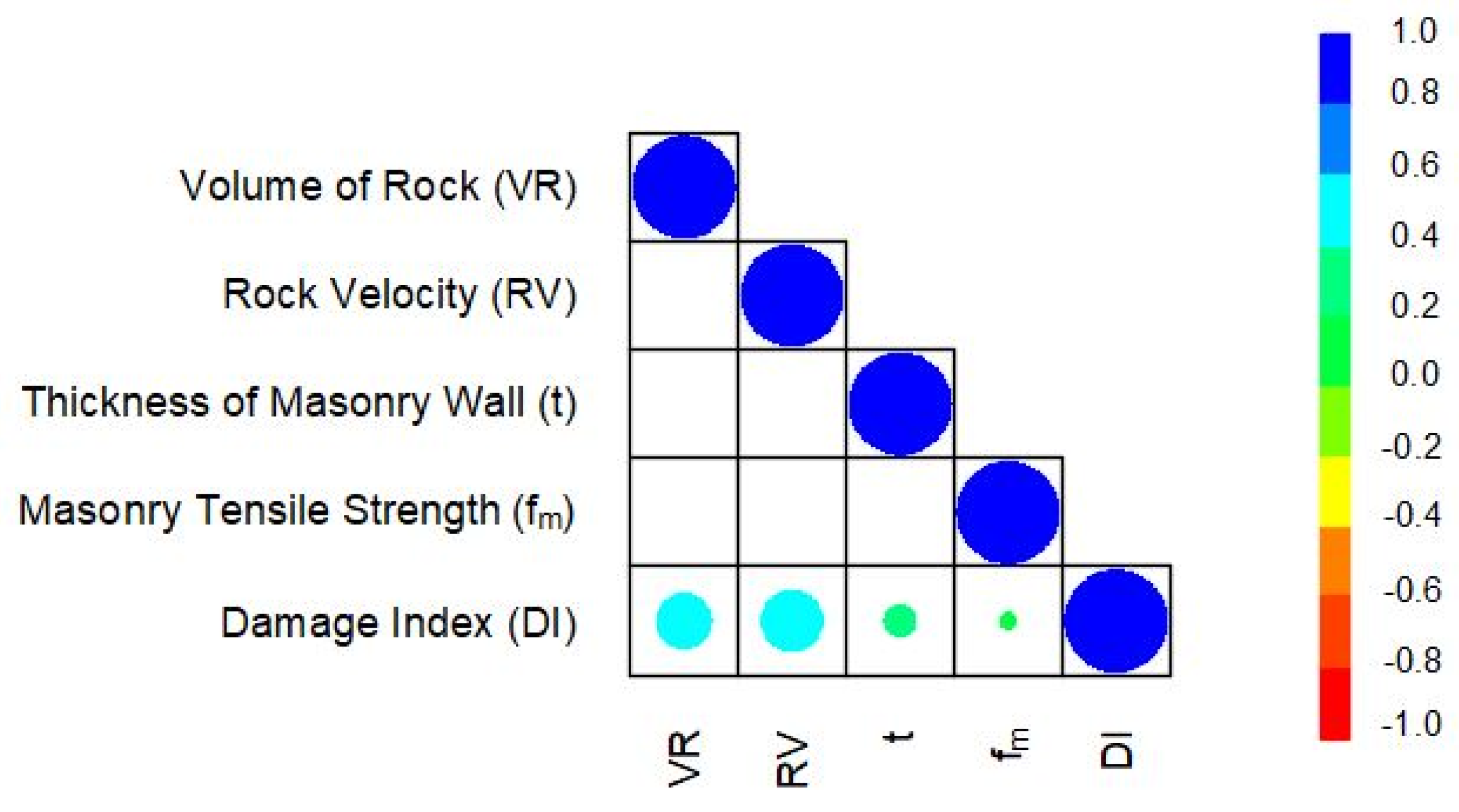
Damage Index	DI	%	Output	0.00	71.00	99.72	27.06	0.38

, the statistical indices for the four input parameters are presented, as well as for the output parameter. Moreover, in Table 2 and in Figure 5 the Pearson correlation coefficients (R) are presented. The values of the last row of this matrix refer to the degree of correlation of the output parameter with each of the other four input parameters. According to this table, it is indicated that the value of the DI is in strong dependence of the rock velocity (R = 0.596) and the rock volume (R = 0.534), followed by the value of wall thickness (R = 0.304), while the smallest correlation is that with the masonry tensile strength (R = 0.151).

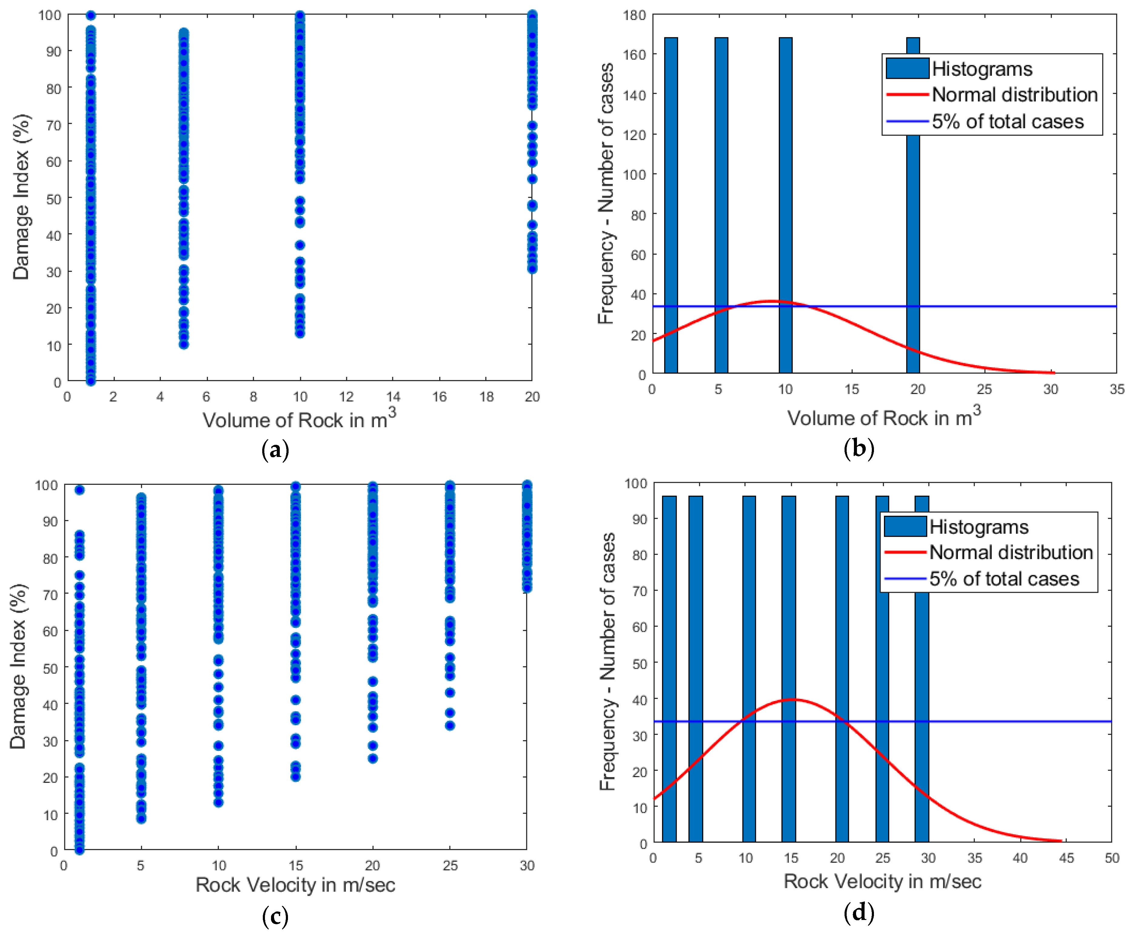
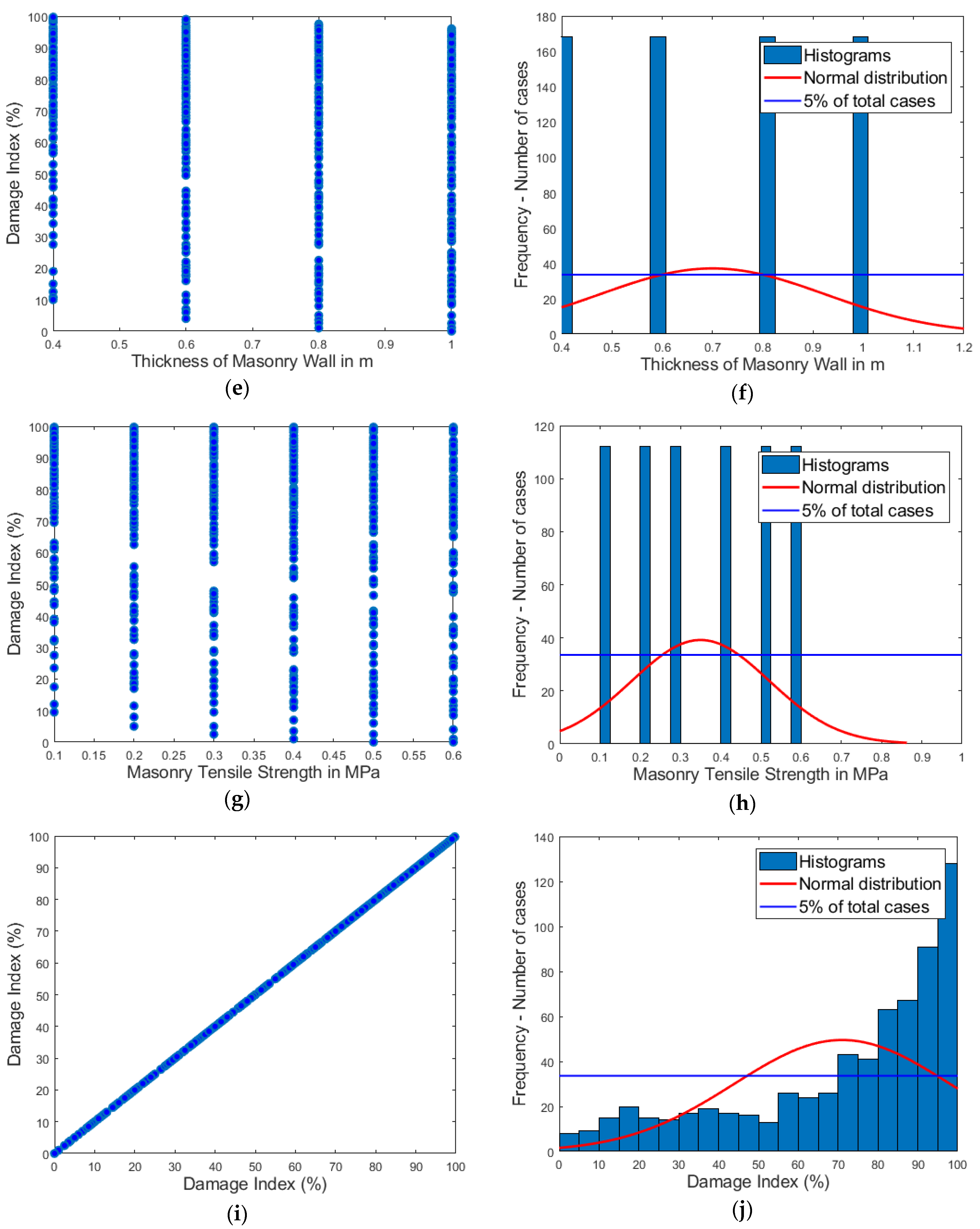
In Figure 6 the histograms and the scatter plots of the used input and output parameters of the database are presented. They indicate the correlation capability of the database and the value ranges for each parameter. They also show where the data are deficient and where the database should be updated in order to achieve greater reliability and completeness.

4.2. Artificial Neural Networks

In 1958, psychologist Frank Rosenblatt [54] formulated and proposed the neural network architecture as an artificial intelligence mathematical model, whose structure resembles the functionality of biological neurons in the brain of mammals. In this first work, the perceptron simulant was proposed, which was the first introduced structure of artificial neural network. The perceptron structure achieved to simulate how the human brain interprets optical sensory input and is able to learn recognizing objects. Even if it was the first one to be proposed, it comprised the main architecture basis for the vast majority of the neural networks that have been introduced and used extensively in all scientific areas.

Perceptron marked a historical turning point in our artificial intelligence timeline and coined a term that was proved to incorporate an entire area within AI. These AI methodologies come as a product of a technological era where a multitude of complex problems with strongly non-linear characteristics are not amenable to solution using classical methods, such as regression and least-squares optimization. Despite the innovation introduced by this architecture, more than four decades were necessary until the nineties, when neural networks were used widely, beginning with medical applications [55,56,57,58,59,60,61,62,63] and followed by computational engineering [64,65,66,67,68,69,70,71,72,73,74].

The structure of an artificial neural network is comprised of a clique of nodes that are interconnected as the biological neurons do, in a way that was inspired by the central nervous system (CNS), whose elementary functions are simulated at each node. Each node in the network is fed with a set of arithmetical inputs from different sources (from other neurons or the environment). A computation is executed using these inputs and an output is produced. This output is provided to the environment or is fed as input to other neurons in the network. Given the nature of the topology of the network three basic types of neurons are distinguished: input neurons, output neurons, and computational or hidden neurons.

The input neurons do not perform any computations, they simply accept the environmental inputs of the network. The computational neurons have the same structure and functionality as the Perceptron. They multiply each input by the respective synaptic weight, they calculate the total sum of products, and they add the bias. This sum is applied as argument to the activation function, which each node implements internally.

More precisely a conventional architecture of the feed forward ANN starts with an input layer followed by a single or multiple hidden layer(s) and terminates with the output layer. Each layer contains an array of nodes and each node receives inputs from nodes of the previous layer, forms a weighted sum, adds a bias, and then transforms them by an activation function to obtain its own output signal. Detailed and in-depth state-of-the-art reports on ANNs can be found in [75,76].

4.3. Performance Indices for the Assessment of Soft Computing Forecasting Models

For the assessment of the effectiveness and the reliability of the computational predictive mathematical simulants, a multitude of statistical indices has been proposed. In

Table 3. Statistical performance indices.

Performance Index	Analytical Formula	Ideal Values
Mean Absolute Error (MAE)	$\mathrm{MAE}=\frac{1}{\mathrm{n}}{\displaystyle {\displaystyle \sum }_{\mathrm{i}=1}^{\mathrm{n}}}\left|\left({\tilde{\mathrm{y}}}_{\mathrm{i}}{}_{\mathrm{i}}-{\mathrm{y}}_{\mathrm{i}}\right)\right|$	0
Mean Absolute Percentage Error (MAPE)	$\mathrm{MAPE}=\frac{1}{\mathrm{n}}{\displaystyle {\displaystyle \sum }_{\mathrm{i}=1}^{\mathrm{n}}}\left|\frac{{\mathrm{y}}_{\mathrm{i}}-{\tilde{\mathrm{y}}}_{\mathrm{i}}}{{\mathrm{y}}_{\mathrm{i}}}\right|\times 100$	0
Root Mean Squared Error (RMSE)	$\mathrm{RMSE}=\sqrt{\frac{1}{\mathrm{n}}{\displaystyle {\displaystyle \sum }_{\mathrm{i}=1}^{\mathrm{n}}}{({\mathrm{y}}_{\mathrm{i}}-{\tilde{\mathrm{y}}}_{\mathrm{i}})}^2}$	0
Variance Account For (VAF)	$\mathrm{VAF}=\left(1-\frac{\mathrm{var}({\mathrm{y}}_{\mathrm{i}}-{\tilde{\mathrm{y}}}_{\mathrm{i}})}{\mathrm{var}({\mathrm{y}}_{\mathrm{i}})}\right)\times 100$	100
Pearson correlation coefficient, also known as Pearson’s r (R)	$\mathrm{R}=\sqrt{\frac{{{\displaystyle \sum }}_{\mathrm{i}=1}^{\mathrm{n}}{({\mathrm{y}}_{\mathrm{i}}-{\mathrm{y}}_{\mathrm{avg}})}^2-{{\displaystyle \sum }}_{\mathrm{i}=1}^{\mathrm{n}}{({\mathrm{y}}_{\mathrm{i}}-{\tilde{\mathrm{y}}}_{\mathrm{i}})}^2}{{{\displaystyle \sum }}_{\mathrm{i}=1}^{\mathrm{n}}{({\mathrm{y}}_{\mathrm{i}}-{\mathrm{y}}_{\mathrm{mean}})}^2}}$	1
alpha 10 (a10-index)	$\mathrm{a}10-\mathrm{index}=\frac{\mathrm{m}10}{\mathrm{n}}$	1

where ${\mathrm{y}}_{\mathrm{i}}$ and ${\hat{\mathrm{y}}}_{\mathrm{i}}$ represent actual and modelled ith value, $\mathrm{n}$ is the sample numbers, ${\mathrm{y}}_{\mathrm{mean}}$ is the average of actual values, and m10 is the number of datasets with value of rate experimental (true) to predicted value between 0.90 and 1.10.

, the most important and widely accepted performance indices of the effectiveness of the forecasting mathematical models are presented [77,78,79,80,81,82,83,84,85,86,87]. Among these, the most spread is the Pearson’s correlation factor R that also exhibits significant weaknesses, mainly if embodied in the code. Among its weaknesses is that besides taking its value into account (the more it tends to one, the better is the respective mathematical predictive model), its inclination angle should also be considered (the more it tends to 45°, the better is the predictive model). With respect to that, an extreme example is given, where a model irrespectively from the values of the input parameters, provides the same output value. In this case the value of the index R is equal to one, while at the same time the slope of the line is zero.

With the aim of a better and also more reliable assessment of the performance of the predictive mathematical models, an index has been proposed recently [88,89], known as the a10-index (last equation in Table 3) that has gained wide acceptance in the recent years [90,91,92,93,94,95,96,97]. This index has the advantage of being understandable and comprehensible, as it has a physical interpretation. It is defined as the percentage of datasets for which the deviation between true and predicted value is less than 10%. The a20-index has been also proposed mainly in the case of experimental databases being used for the training of surrogate models. The deviation between true and predicted value for the a20-index is less than 20%. A detailed and in-depth state-of-the-art report on performance indices for the assessment of soft computing forecasting mathematical models can be found in [98,99,100,101,102,103].

5. Results and Discussion

5.1. Training and Development of ANN Models

In order to identify the optimal ANN model for the prediction of rockfall failure of masonry walls, different architectures of ANN models have been trained and developed. It is well-known that the method of artificial neural networks is an inherently heuristic method and, accordingly, the involved parameters such as the number of neurons per hidden layer, the transfer functions, the optimization algorithms, the data normalization techniques, and the possible combinations of these are of huge cardinality. For the present study, the following steps were included:

• Splitting of the database into training, validating, and testing datasets. The splitting of the database affects significantly the reliability of the developed mathematical model. The splitting took place so as to have, as much as possible, equal distribution for all the parameters, as well as to achieve a minimum deviation of the performance indices values, for both the training and testing datasets. In the present study, the 672 datasets were split into 448 training (66.66%), 112 validating (16.67%), and 112 testing (16.67%) datasets. The databases used for the training and the development of the ANN models are appended as Supplementary Materials in the excel file titled Database.xls.
• Selection of training algorithms. For the training of the AΝΝ models, six different optimization algorithms were selected, which are presented in

  Table 4. Optimization algorithms for the training and development of ANN models applied in this study.

  Nr.	Algorithm	Matlab Function	Abbreviation
  1	Levenberg–Marquardt Algorithm [93,94,95,96]	trainlm	LM
  2	Gradient descent backpropagation [97]	traingd	GD
  3	Gradient descent with momentum backpropagation [97]	traingdm	GDM
  4	Gradient descent with momentum and adaptive learning rate backpropagation [97]	traingdx	GDX
  5	Scaled conjugate gradient backpropagation [97,98]	trainscg	SCG
  6	Broyden–Fletcher–Goldfarb–Shanno (BFGS) quasi-Newton backpropagation [99,100,101,102]	trainbfg	BFGS

  .
• Normalization of data. For the normalization of data, four (4) different normalization techniques including minmax and z-score techniques were used (

  Table 5. Training parameters of ANN models applied in this study.

  Parameter	Value	Matlab Function(s)
  Training Algorithm	Six different optimization algorithms (See Table 5)
  Data splitting	Ten different cases based on ten different random generation numbers
  Normalization	Without any normalization Minmax in the range [0.10–0.90], [0.00–1.00] and [−1.00–1.00] Zscore	Mapminmax zscore
  Number of Hidden Layers	1
  Number of Neurons per Hidden Layer	1 to 50 by step 1
  Control random number generation	Ten different random generation	rand(seed, generator), where the generator range from 1 to 10 by step 1
  Training Goal	0
  Maximum Number of Epochs	200
  Cost Function	Mean Square Error (MSE)	mse
  	Sum Square Error (SSE)	sse
  Transfer Functions	Hyperbolic Tangent Sigmoid transfer function (HTS)	tansig
  	Log-sigmoid transfer function (LS)	logsig
  	Linear transfer function (Li)	purelin
  	Positive linear transfer function (PLi)	poslin
  	Symmetric saturating linear transfer function (SSL)	satlins
  	Soft max transfer function (SM)	softmax
  	Competitive transfer function (Co)	compet
  	Triangular basis transfer function (TB)	tribas
  	Radial basis transfer function (RB)	radbas
  	Normalized radial basis transfer function (NRB)	radbasn
  	Hard-limit transfer function (HL)	hardlim
  	Symmetric hard-limit transfer function (SHL)	hardlims

  ).
• Activation functions. For each ANN architecture, twelve (12) different transfer functions were used (Table 5). These correspond to 144 (12 × 12) different combinations for each ANN architecture with one hidden layer, and accordingly to 1728 (12 × 12 × 12) combinations in the case of ANNs with two hidden layers.

Considering all the parameters presented in Table 4 and Table 5, 3,456,000 different ANN models were trained and developed. These models were ranked according to their performance. The best 20 models are presented in

Table 6. Best twenty optimum architectures of ANN models based on testing datasets RMSE index.

Ranking	Algorithm	Normalization Technique	Cost Function	Transfer Function		Architecture	Datasets Performance Indices
				Input Layer	Output Layer		Testing		Training		All
							R	RMSE	R	RMSE	R	RMSE
1	LM	Minmax [0.00, 1.00]	MSE	NRB	HTS	4-21-1	0.9995	0.8081	0.9996	0.7868	0.9994	0.9671
2	LM	Minmax [0.00, 1.00]	MSE	NRB	RB	4-34-1	0.9995	0.8354	0.9997	0.6537	0.9995	0.9008
3	LM	Minmax [0.00, 1.00]	MSE	NRB	HTS	4-27-1	0.9995	0.8602	0.9996	0.7280	0.9993	1.0337
4	LM	Minmax [0.10, 0.90]	SSE	HTS	SSL	4-42-1	0.9995	0.8634	0.9998	0.5505	0.9995	0.8414
5	LM	Minmax [0.10, 0.90]	MSE	NRB	HTS	4-24-1	0.9995	0.8644	0.9995	0.8194	0.9989	1.2777
6	LM	Minmax [0.00, 1.00]	MSE	HTS	HTS	4-25-1	0.9995	0.8654	0.9997	0.6288	0.9995	0.8444
7	LM	Zscore	MSE	HTS	Li	4-35-1	0.9995	0.8684	0.9997	0.6253	0.9994	0.9555
8	LM	Minmax [0.10, 0.90]	SSE	NRB	LS	4-23-1	0.9995	0.8693	0.9996	0.7422	0.9994	0.9536
9	LM	Minmax [0.00, 1.00]	MSE	LS	LS	4-28-1	0.9995	0.8706	0.9998	0.5918	0.9994	0.9680
10	LM	Minmax [0.00, 1.00]	MSE	HTS	PLi	4-45-1	0.9995	0.8718	0.9999	0.4541	0.9994	0.9201
11	LM	Minmax [0.00, 1.00]	MSE	LS	LS	4-22-1	0.9995	0.8720	0.9996	0.7678	0.9993	1.0018
12	LM	Minmax [0.10, 0.90]	SSE	HTS	HTS	4-46-1	0.9995	0.8722	0.9997	0.6828	0.9973	1.9940
13	LM	Minmax [0.10, 0.90]	SSE	HTS	LS	4-32-1	0.9995	0.8748	0.9997	0.6752	0.9993	1.0328
14	LM	Minmax [0.00, 1.00]	SSE	HTS	HTS	4-25-1	0.9995	0.8752	0.9996	0.7647	0.9994	0.9680
15	LM	Minmax [0.10, 0.90]	SSE	NRB	HTS	4-26-1	0.9995	0.8756	0.9996	0.7151	0.9994	0.9707
16	LM	Minmax [0.00, 1.00]	SSE	HTS	LS	4-36-1	0.9995	0.8756	0.9998	0.5441	0.9994	0.9381
17	LM	Minmax [0.10, 0.90]	MSE	NRB	SSL	4-35-1	0.9995	0.8758	0.9997	0.6646	0.9989	1.2517
18	LM	Minmax [0.10, 0.90]	SSE	NRB	HTS	4-33-1	0.9995	0.8772	0.9998	0.5607	0.9995	0.8885
19	LM	Minmax [0.00, 1.00]	MSE	NRB	Li	4-35-1	0.9995	0.8778	0.9998	0.4932	0.9995	0.8455
20	LM	Zscore	MSE	SM	Li	4-31-1	0.9995	0.8786	0.9998	0.5436	0.9995	0.8279

. The set of the best 20 ANN models corresponds to the models trained by the Levenberg–Marquardt Algorithm [104,105,106,107]. It is also indicated that the minmax normalization technique dominates. In

Table 7. Optimal ANN architectures for the six different algorithms used for the optimization of ANN models.

Ranking	Algorithm	Normalization Technique	Cost Function	Transfer Function		Architecture	Datasets Performance Indices
				Input Layer	Output Layer		Testing		Training		All
							R	RMSE	R	RMSE	R	RMSE
1	LM	Minmax [0.00, 1.00]	MSE	NRB	HTS	4-21-1	0.9995	0.8081	0.9996	0.7868	0.9994	0.9671
2	BFGS	Minmax [−1.00, 1.00]	SSE	NRB	HTS	4-28-1	0.9994	0.9255	0.9996	0.7830	0.9993	0.9982
3	SCG	Zscore	SSE	RBn	Li	4-27-1	0.9991	1.1463	0.9990	1.1684	0.9986	1.4210
4	GDM	Minmax [−1.00, 1.00]	SSE	TB	HTS	4-27-1	0.9949	2.9277	0.9939	2.9486	0.9926	3.3273
5	GDX	Zscore	SSE	TB	Li	4-26-1	0.9938	3.0616	0.9937	3.0540	0.9929	3.2752
6	GD	Minmax [0.00, 1.00]	SSE	TB	LS	4-18-1	0.9764	5.9139	0.9733	6.1335	0.9700	6.6204

, the best ANN models for each one of the six different training algorithms are presented. The second-best training algorithm is the Broyden–Fletcher–Goldfarb–Shanno (BFGS) quasi-Newton backpropagation algorithm [107,108,109,110].

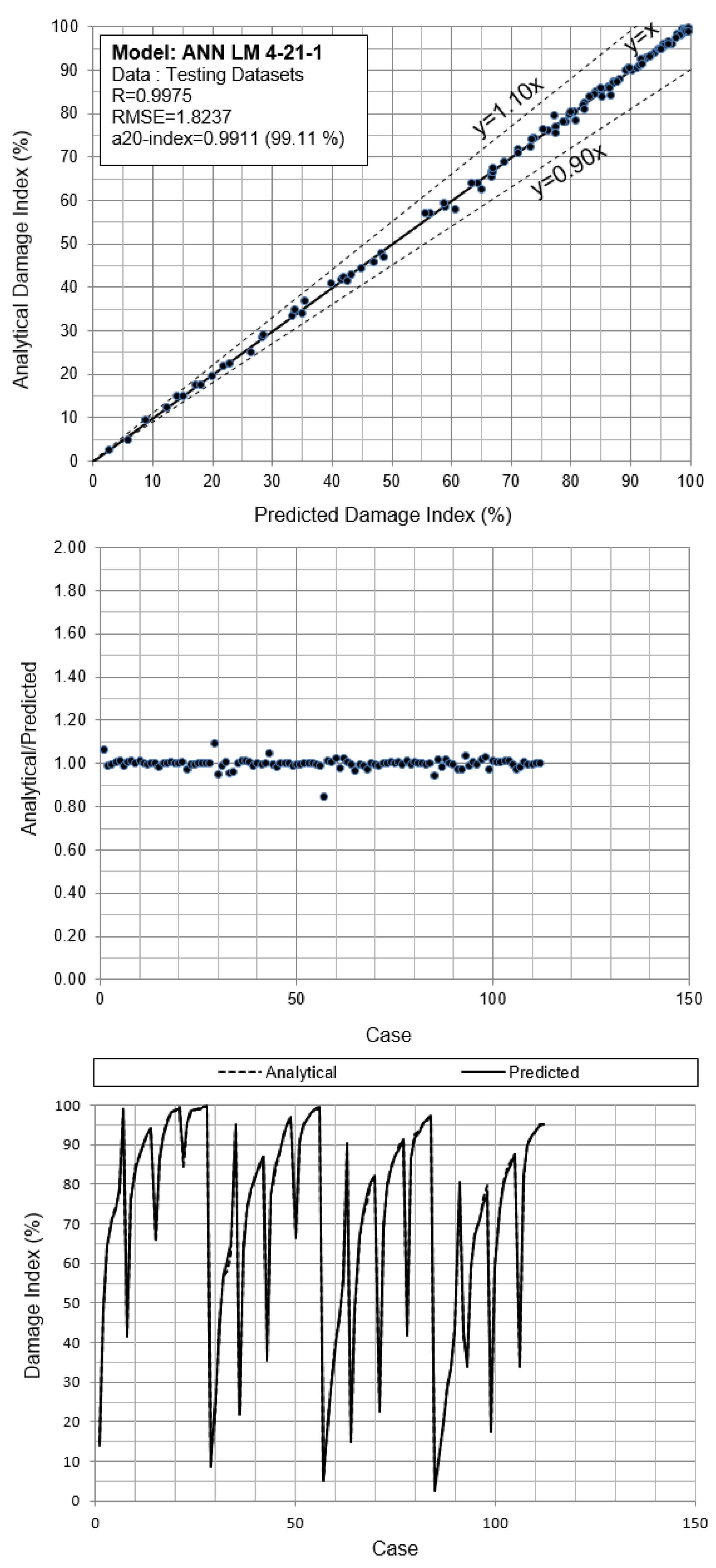
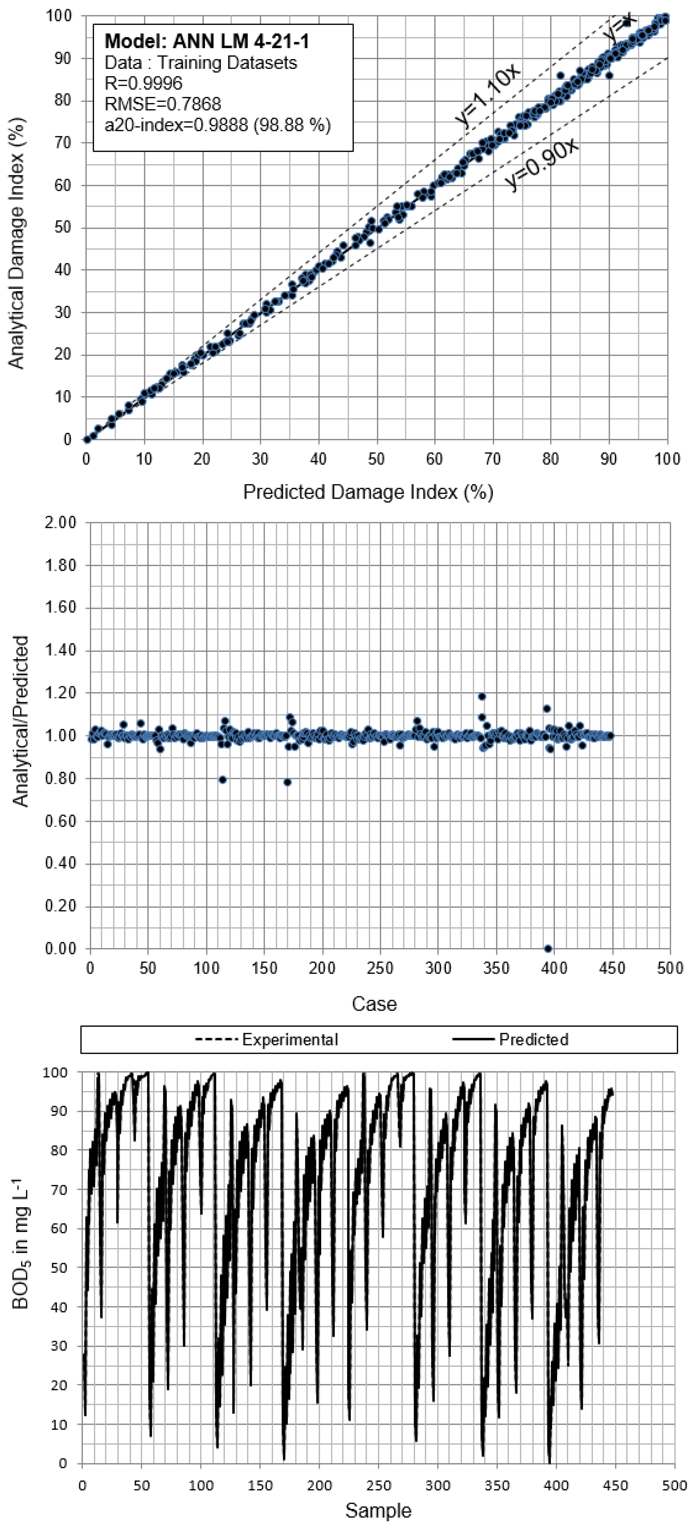
Based on the above, the optimum ANN model is the ANN LM 4-21-1 model (

Table 8. Summary of prediction capability of the optimum ANN LM 4-21-1 model.

Model	Datasets	Performance Indices
		a10-index	R	RMSE	MAPE	VAF
ANN LM 4-21-1	Training	0.9888	0.9996	0.7868	0.0144	99.9115
	Test	0.9911	0.9995	0.8081	0.0128	99.9099

) which has 24 neurons, and has been optimized by the Levenberg–Marquardt algorithm, and the mean square error (MSE) is as a cost function. Data normalization has been performed with the minmax technique. The normalized radial basis transfer function (NRB) has been used for the input layer and the Hyperbolic Tangent Sigmoid transfer function (HTS) for the output layer. The optimal ANN LM 4-21-1 model achieved almost ideal values of the performance indices (Table 8). The validation results are also shown in Figure 7 and Figure 8 where the analytical vs predicted values of the damage index for the testing and training datasets are presented.

5.2. Closed-Form Equation for the Estimation of Damage Index

In the previous sub-section, the architecture of the proposed ANN LM 4-21-1 model for the prediction of the damage index of masonry walls under rockfalls was presented. The input parameter weights and biases are also provided, so that other researchers and practitioners can verify the reliability of the proposed model.

Under the prism of the above considerations, Equation (8) describes analytically the proposed ANN LM 4-21-1 model and can be used for the estimation of the damage index of masonry structures under rockfalls as a function of the input parameters: the rock volume (VR), the rock velocity (RV), the thickness of masonry wall (t), and the masonry tensile strength ${\mathrm{f}}_{\mathrm{m}}$:

$${\mathrm{DI}}_{\mathrm{norm}}=\tan \mathrm{sig}\left(\left[\mathrm{LW}\left\{2,1\right\}\right]\times \left[\mathrm{radbasn}\left(\left[\mathrm{IW}\left\{1,1\right\}\right]\times \left[\mathrm{IP}\right]+\left[\mathrm{B}\left\{1,1\right\}\right]\right)\right]+\left[\mathrm{B}\left\{2,1\right\}\right]\right)$$

(8)

$${\mathrm{DI}}_{\mathrm{real}}=\frac{\left({\mathrm{DI}}_{\mathrm{norm}}-\mathrm{a}\right)\times \left({\mathrm{DI}}_{\max }-{\mathrm{DI}}_{\min }\right)}{\mathrm{b}-\mathrm{a}}+{\mathrm{DI}}_{\min }$$

(9)

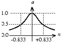
where a = 0.00 and b = 1.00 are the lower and upper limits of the minmax normalization technique applied on the data, ${\mathrm{DI}}_{\max }$ = 99.72 and ${\mathrm{DI}}_{\min }$ = 0.00 are the maximum and minimum values of the damage index present in the database, that was used for the training of the ANN models. The tansig and radbasn are the hyperbolic tangent sigmoid transfer function (HTS) and the normalized radial basis transfer function (NRB), respectively. Their details (equations and graphs) are presented in

Table 9. Transfer functions used in the optimum proposed ANN LM 4-21-1 model.

SN	Transfer Function/Equation/Matlab Function	Graph
1	The normalized radial basis transfer function (NRB)
	$\mathrm{a}=\frac{\exp \left(-{\mathrm{n}}^2\right)}{\mathrm{sum}\left(\exp \left(-{\mathrm{n}}^2\right)\right)}$
	$\mathrm{a}=\mathrm{f}\left(\mathrm{n}\right)=\mathrm{radbasn}\left(\mathrm{n}\right)$
2	The hyperbolic tangent sigmoid transfer function (HTS)
	$\mathrm{a}=\mathrm{f}\left(\mathrm{n}\right)=\frac{2}{1+\exp \left(-2\hspace{0.17em}\ast \hspace{0.17em}\mathrm{n}\right)}-1$
	$\mathrm{a}=\mathrm{f}\left(\mathrm{n}\right)=\tan \mathrm{sig}\left(\mathrm{n}\right)$

.

Equation (9) describes the proposed ANN LM 4-21-1 model in a purely mathematical form so that its reproduction becomes straightforward. In Equation (8), $\left[\mathrm{IW}\left\{1,1\right\}\right]$ is a 21 $\times$ 4 matrix that contains the weights of the hidden layer; $\left[\mathrm{LW}\left\{2,1\right\}\right]$ is a 1 $\times$ 21 vector with the weights of the output layer; $\left[\mathrm{IP}\right]$ is a 4 × 1 vector with the four (4) input variables; $\left[\mathrm{B}\left\{1,1\right\}\right]$ is a 21$\times$1 vector that contains the bias values of the hidden layer; and $\left[\mathrm{B}\left\{2,1\right\}\right]$ is a 1 $\times$ 1 vector with the bias of the output layer. The $\left[\mathrm{IP}\right]$ vector consists of the four (4) normalized values of the input variables of the rock volume (VR), the rock velocity (RV), the thickness of masonry wall (t), and the masonry tensile strength ${\mathrm{f}}_{\mathrm{m}}$. IP is defined by:

$$\left[\mathrm{IP}\right]=\left[\begin{array}{c}\mathrm{a}+\left(\mathrm{b}-\mathrm{a}\right)\left(\frac{\mathrm{VR}-\min \left(\mathrm{VR}\right)}{\max \left(\mathrm{VR}\right)-\min \left(\mathrm{VR}\right)}\right)\\ \mathrm{a}+\left(\mathrm{b}-\mathrm{a}\right)\left(\frac{\mathrm{RV}-\min \left(\mathrm{RV}\right)}{\max \left(\mathrm{RV}\right)-\min \left(\mathrm{RV}\right)}\right)\\ \begin{array}{c}\mathrm{a}+\left(\mathrm{b}-\mathrm{a}\right)\left(\frac{\mathrm{t}-\min \left(\mathrm{t}\right)}{\max \left(\mathrm{t}\right)-\min \left(\mathrm{t}\right)}\right)\\ \mathrm{a}+\left(\mathrm{b}-\mathrm{a}\right)\left(\frac{{\mathrm{f}}_{\mathrm{m}}-\min \left({\mathrm{f}}_{\mathrm{m}}\right)}{\max \left({\mathrm{f}}_{\mathrm{m}}\right)-\min \left({\mathrm{f}}_{\mathrm{m}}\right)}\right)\end{array}\end{array}\right]$$

(10)

where the $\min \left(\mathrm{VR}\right)$ = 1.00, $\max \left(\mathrm{VR}\right)$ = 20.00; $\min \left(\mathrm{RV}\right)$ = 1.00, $\max \left(\mathrm{RV}\right)$ = 30.00; $\min \left(\mathrm{t}\right)$ = 0.40, $\max \left(\mathrm{t}\right)$ = 1.00; and $\min \left({\mathrm{f}}_{\mathrm{m}}\right)$ = 0.10, $\max \left({\mathrm{f}}_{\mathrm{m}}\right)$ = 0.60 are the lower and higher values of the input parameters (Table 2). The values of the final weights and biases that determine the matrices $\left[\mathrm{IW}\left\{1,1\right\}\right]$, $\left[\mathrm{LW}\left\{2,1\right\}\right]$, $\left[\mathrm{B}\left\{1,1\right\}\right]$, and $\left[\mathrm{B}\left\{2,1\right\}\right]$ are presented in

Table 10. Final values of weights and bias of the ANN-LM 4-21-1 model.

IW{1,1}				${\left[\mathbf{LW}\left\{2,1\right\}\right]}^{\mathbf{T}}$	$\left[\mathbf{B}\left\{1,1\right\}\right]$	$\left[\mathbf{B}\left\{2,1\right\}\right]$
(21 × 4)				(1 × 21)	(21 × 1)	(1 × 1)
−0.3652	0.9489	−2.9307	0.9458	−1.3912	1.7557	1.5653
1.7306	1.3115	7.7442	0.8606	−1.0532	−9.5504
−16.6491	18.5646	−16.2404	−0.1639	−0.1469	19.8556
−1.2270	−0.6461	2.2374	0.2739	4.5887	1.4360
−0.0602	0.6190	−0.1182	−0.0056	22.3429	−1.7328
−0.0483	−0.7170	0.8289	2.6856	0.8243	0.7565
1.7158	−2.4048	−4.8431	−0.3589	−1.0335	0.7911
−0.3454	−2.5670	0.7348	−0.7525	−0.6348	1.3841
5.5504	19.0378	−2.2654	−0.9111	−0.7584	−4.5451
4.0931	−5.0231	1.9202	0.0946	−0.5279	−0.6546
4.2287	−2.0062	−2.1430	−0.3746	−1.0895	0.5203
3.9949	4.2281	−1.2621	−0.4834	−2.4858	0.3005
1.5895	2.2236	−2.0486	−0.0550	0.5094	−0.8105
−1.5270	0.0059	−1.5890	1.3683	−1.2488	0.1031
0.6285	−7.4145	−1.1262	0.0401	−4.1664	−0.5063
−8.4275	2.3670	0.2385	0.8626	0.5009	−0.3484
6.8743	3.1965	0.6128	0.4617	0.4097	−2.0923
−0.6447	2.0363	−2.5711	0.6641	−1.3161	−0.2042
−3.9182	3.0640	0.5657	0.3649	−2.7053	−1.9747
−7.8553	8.6296	0.0836	0.0502	−3.5478	−6.7058
−3.1907	−0.4128	−0.1650	0.4660	−4.5351	−0.2191

Note: $\left[\mathrm{IW}\left\{1,1\right\}\right]$ is the matrix of weight values between the input layer and the first hidden layer; $\left[\mathrm{LW}\left\{2,1\right\}\right]$ is the matrix of weight values between the first hidden layer and the output layer; $\left[\mathrm{B}\left\{1,1\right\}\right]$ is the matrix of bias values for the hidden layer, and $\left[\mathrm{B}\left\{2,1\right\}\right]$ is the matrix of bias values for the output layer.

.

5.3. Mapping of Rockfall Masonry Wall Damage Index

To provide a friendly to use tool for estimating the rockfall damage of masonry walls, and the vulnerability values to be imported into the rockfall risk equation, a series of charts is provided (Figure 9 and Figure 10). The reliability of the proposed model is further supported by the observed smoothness of all the graphed curves, which indicates that there is no overfitting.

Figure 9 and Figure 10 show the DI contours for two selected sizes of blocks, 5 m³ and 10 m³, for which the variability of the DI according to the input parameters can be observed. For the larger blocks, the variability of the DI is smaller. The relation between the DI and the wall width as well as with the masonry tensile strength is almost linear for 5 m³, while for 10 m³ this linearity is not observed. The wall thickness has an important effect on decreasing the DI for lower velocities and blocks up to 5 m³. For higher velocities and bigger rock blocks, this effect is less apparent as the DI tends to be over 80%. The effect of the masonry tensile strength, depending on the mortar strength and the wall units is also an important parameter to be considered for the DI. However, in practice, for the vulnerability assessment, this parameter is difficult to be estimated with accuracy.

6. Limitations and Future Work

Limitations of this work come at different stages of the analysis. Concerning the use of the proposed DI for the vulnerability at the risk equation, it has to be taken into account that this value refers to the initial impact onto a building, and that it does not take into account the propagation of the rock into the building, a potential collapse of the building due to loss of its overall stability, nor non-structural damage.

Limitations of this work with respect to the determination of the contact forces concern the non-conservative assumption of cubic block shape and of full rock-wall contact during the impact. A fixed Young’s modulus was considered for the rock block, thus lithology variation is not considered here. Nevertheless, this can be further investigated using the proposed methodology. Moreover, the basic assumption of a rock moving horizontally and impacting the wall with a horizontal velocity was made. Falling rocks or rocks impacting the wall with a given incidence angle have not been considered here. In the same way, only the kinetic energy of the rock block was simulated and further studies are needed in order to determine which is the real effect of the boulder rotation in the characterization of the impact.

The assessment of the out-of-plane response of the masonry can be improved using solid finite elements, and specific failure criteria for the out-of-plane shear stress of the wall. Different assumptions concerning the wall boundary conditions (in this work the wall was considered fixed at the base and hinged at the top) and their effect on the damage can also be investigated in the future. Moreover, the provided simulations address non-load-bearing walls, without considering how the response of the masonry wall would change in function of different vertical overlying weights.

Each computational predictive model is reliable only for the range of values of parameters that comprise the database that was used for its training and development. The proposed ANN LM 4-21-1 model can provide reliable predictions for values of the input parameters between the minimum and maximum value of each parameter as defined in Table 2. For values out of these ranges, each prediction is risky because the proposed model has not been trained accordingly. To enlarge the range of validity of the proposed model, the authors plan to update the database. With respect to that, there is a double requirement for the damage database. First, it should be extended to include different masonry types, dimensions, and mechanical properties. A next step would be to interpret the mechanical properties of the masonry and specifically the wall tensile strength into categorical masonry classes (for instance according to age, materials etc.,).

7. Conclusions

A numerical methodology has been provided for assessing the expected damage for masonry walls when impacted by rock blocks, in terms of a DI. A large database of 672 datasets has been created as a tank of damage values. The database includes four input parameters, two characterizing the masonry wall (wall width and tensile strength) and two the rock block kinematics (rock block volume and velocity).

Based on this database, a variety of AI algorithms has been tested to provide the optimum model describing the DI. The optimal model to calculate the expected DI was the ANN LM 4-21-1 model. Using this model, the a10-index was 0.9888 for the training and 0.9911 for the test data. The R index was calculated to be 0.9996 and 0.9995, respectively. The fitted curves were observed to be smooth, which indicates that there is no overfitting. Both the wall width and the masonry tensile strength were indicated to have an important effect on the resultant damage. Neglecting them during the risk analysis could lead to non-reliable results.

According to the selected AI model, an equation was extracted for the calculation of the DI, which can be directly incorporated into the risk assessment equation. The application constraints for the provided results, concerning database limitations and difficulties for the characterization of the structural typology, should be taken into consideration, as described in Section 6. Further comparison with real cases is needed for the verification of the results of this work, which is possible using the proposed equation.

References

1. Lanzo, G.; Tommasi, P.; Ausilio, E.; Aversa, S.; Bozzoni, F.; Cairo, R.; D’onofrio, A.; Durante, M.G.; Foti, S.; Giallini, S.; et al. Reconnaissance of geotechnical aspects of the 2016 Central Italy earthquakes. Bull. Earthq. Eng. 2018, 17, 5495–5532. [Google Scholar] [CrossRef]
2. Corominas, J.; Mavrouli, O. Rockfall Quantitative Risk Assessment in Rockfall Engineering; Lambert, S., Nicot, F., Eds.; Wiley Online Library: Hoboken, NJ, USA, 2013; pp. 255–301. [Google Scholar]
3. Scavia, C.; Barbero, M.; Castelli, M.; Marchelli, M.; Peila, D.; Torsello, G.; Vallero, G. Evaluating rockfall risk: Some critical aspects. Geosciences 2020, 10, 98. [Google Scholar] [CrossRef]
4. Papathoma-Köhle, M.; Kappes, M.; Keiler, M.; Glade, T. Physical vulnerability assessment for alpine hazards: State of the art and future needs. Nat. Hazards 2011, 58, 645–680. [Google Scholar] [CrossRef]
5. Agliardi, F.; Crosta, G.B.; Frattini, P. Integrating rockfall risk assessment and countermeasure design by 3D modelling techniques. Nat. Hazards Earth Syst. Sci. 2009, 9, 1059–1073. [Google Scholar] [CrossRef]
6. Grant, A.; Wartman, J.; Massey, C.; Olsen, M.J.; O’Banion, M.; Motley, M. The impact of rockfalls on dwellings during the 2011 Christchurch, New Zealand, earthquakes. Landslides 2018, 15, 31–42. [Google Scholar] [CrossRef]
7. Yang, J.; Duan, S.; Li, Q.; Liu, C. A Review of Flexible Protection in Rockfall Protection. Nat. Hazards 2019, 99, 71–89. [Google Scholar] [CrossRef]
8. Fotopoulou, S.D.; Pitilakis, K.D. Fragility curves for reinforced concrete buildings to seismically triggered slow-moving slides. Soil Dyn. Earthq. Eng. 2013, 48, 143–161. [Google Scholar] [CrossRef]
9. Negulescu, C.; Foerster, E. Parametric studies and quantitative assessment of the vulnerability of a RC frame building exposed to differential settlements. Nat. Hazards Earth Syst. Sci. 2010, 10, 1781–1792. [Google Scholar] [CrossRef]
10. Cuomo, S.; Di Perna, A.; Martinelli, M. MPM modelling of buildings impacted by landslides. In Understanding and Reducing Landslide Disaster Risk: Volume 5 Catastrophic Landslides and Frontiers of Landslide Science, 5th ed.; Springer: Berlin/Heidelberg, Germany, 2021; pp. 245–266. [Google Scholar]
11. Mavrouli, O.; Corominas, J. Rockfall vulnerability assessment for reinforced concrete buildings. Nat. Hazards Earth Syst. Sci. 2010, 10, 2055–2066. [Google Scholar] [CrossRef]
12. Vallero, G.; De Biagi, V.; Barbero, M.; Castelli, M.; Napoli, M.L. A method to quantitatively assess the vulnerability of masonry structures subjected to rockfalls. Nat. Hazards 2020, 103, 1307–1325. [Google Scholar] [CrossRef]
13. Mavrouli, O.; Giannopoulos, P.G.; Carbonell, J.M.; Syrmakezis, C. Damage analysis of masonry structures subjected to rockfalls. Landslides 2017, 14, 891–904. [Google Scholar] [CrossRef]
14. Barkhordari, M.S.; Armaghani, D.J.; Asteris, P.G. Structural damage identification using ensemble deep convolutional neural network models. Comput. Model. Eng. Sci. 2023, 134, 835–855. [Google Scholar] [CrossRef]
15. Yari, M.; Armaghani, D.J.; Maraveas, C.; Ejlali, A.N.; Mohamad, E.T.; Asteris, P.G. Several Tree-Based Solutions for Predicting Flyrock Distance Due to Mine Blasting. Appl. Sci. 2023, 13, 1345. [Google Scholar] [CrossRef]
16. Esteva, A.; Kuprel, B.; Novoa, R.A.; Ko, J.; Swetter, S.M.; Blau, H.M.; Thrun, S. Dermatologist-level classification of skin cancer with deep neural networks. Nature 2017, 542, 115–118. [Google Scholar] [CrossRef] [PubMed]
17. Asteris, P.G.; Alexakis, D.E.; Tsoukalas, M.Z.; Gamvroula, D.E.; Guney, D. Machine Learning Approach for Rapid Estimation of Five-Day Biochemical Oxygen Demand in Wastewater. Water 2023, 15, 103. [Google Scholar] [CrossRef]
18. Koopialipoor, M.; Asteris, P.G.; Mohammed, A.M.; Alexakis, D.E.; Mamou, A.; Armaghani, D.J. Introducing stacking machine learning approaches for the prediction of rock deformation. Transp. Geotech. 2022, 34, 100756. [Google Scholar] [CrossRef]
19. Ghanizadeh, A.R.; Ghanizadeh, A.; Asteris, P.G.; Fakharian, P.; Armaghani, D.J. Developing Bearing Capacity Model for Geogrid-Reinforced Stone Columns Improved Soft Clay by Means of MARS-EBS Hybrid Method. Transp. Geotech. 2023, 38, 100906. [Google Scholar] [CrossRef]
20. Le, L.T.; Nguyen, H.; Dou, J.; Zhou, J. A comparative study of PSO-ANN, GA-ANN, ICA-ANN, and ABC-ANN in estimating the heating load of buildings’ energy efficiency for smart city planning. Appl. Sci. 2019, 9, 2630. [Google Scholar] [CrossRef]
21. Zhou, J.; Li, X.; Mitri, H.S. Classification of rockburst in underground projects: Comparison of ten supervised learning methods. J. Comput. Civ. Eng. 2016, 30, 04016003. [Google Scholar] [CrossRef]
22. Indraratna, B.; Armaghani, D.J.; Correia, A.G.; Hunt, H.; Ngo, T. Prediction of resilient modulus of ballast under cyclic loading using machine learning techniques. Transp. Geotech. 2023, 38, 100895. [Google Scholar] [CrossRef]
23. Ashrafian, A.; Panahi, E.; Salehi, S.; Karoglou, M.; Asteris, P.G. Mapping the strength of agro-ecological lightweight concrete containing oil palm by-product using artificial intelligence techniques. Structures 2023, 48, 1209–1229. [Google Scholar] [CrossRef]
24. Tan, W.Y.; Lai, S.H.; Teo, F.Y.; Armaghani, D.J.; Pavitra, K.; El-Shafie, A. Three Steps towards Better Forecasting for Streamflow Deep Learning. Appl. Sci. 2022, 12, 12567. [Google Scholar] [CrossRef]
25. Asteris, P.G.; Nozhati, S.; Nikoo, M.; Cavaleri, L.; Nikoo, M. Krill herd algorithm-based neural network in structural seismic reliability evaluation. Mech. Adv. Mater. Struct. 2019, 26, 1146–1153. [Google Scholar] [CrossRef]
26. Armaghani, D.J.; Asteris, P.G.; Fatemi, S.A.; Hasanipanah, M.; Tarinejad, R.; Rashid, A.S.A.; Huynh, V.V. On the Use of Neuro-Swarm System to Forecast the Pile Settlement. Appl. Sci. 2020, 10, 1904. [Google Scholar] [CrossRef]
27. Shan, F.; He, X.; Armaghani, D.J.; Zhang, P.; Sheng, D. Success and challenges in predicting TBM penetration rate using recurrent neural networks. Tunn. Undergr. Space Technol. 2022, 130, 104728. [Google Scholar] [CrossRef]
28. Asteris, P.G.; Maraveas, C.; Chountalas, A.T.; Sophianopoulos, D.S.; Naveed Alam, N. Fire resistance prediction of slim-floor asymmetric steel beams using single hidden layer ANN models that employ multiple activation functions. Steel Compos. Struct. 2022, 44, 755–774. [Google Scholar]
29. Ghanizadeh, A.R.; Delaram, A.; Fakharian, P.; Armaghani, D.J. Developing Predictive Models of Collapse Settlement and Coefficient of Stress Release of Sandy-Gravel Soil via Evolutionary Polynomial Regression. Appl. Sci. 2022, 12, 9986. [Google Scholar] [CrossRef]
30. Li, C.; Zhou, J.; Tao, M.; Du, K.; Wang, S.; Armaghani, D.J.; Mohamad, E.T. Developing hybrid ELM-ALO, ELM-LSO and ELM-SOA models for predicting advance rate of TBM. Transp. Geotech. 2022, 36, 100819. [Google Scholar] [CrossRef]
31. Hasanipanah, M.; Monjezi, M.; Shahnazar, A.; Armaghani, D.J.; Farazmand, A. Feasibility of indirect determination of blast induced ground vibration based on support vector machine. Measurement 2015, 75, 289–297. [Google Scholar] [CrossRef]
32. Asteris, P.G.; Nikoo, M. Artificial bee colony-based neural network for the prediction of the fundamental period of infilled frame structures. Neural Comput. Appl. 2019, 31, 4837–4847. [Google Scholar] [CrossRef]
33. Asteris, P.G.; Mamou, A.; Hajihassani, M.; Hasanipanah, M.; Koopialipoor, M.; Le, T.-T.; Kardani, N.; Armaghani, D.J. Soft computing based closed form equations correlating L and N-type Schmidt hammer reboundnumbers of rocks. Transp. Geotech. 2021, 29, 100588. [Google Scholar] [CrossRef]
34. Asteris, P.G.; Ashrafian, A.; Rezaie-Balf, M. Prediction of the Compressive Strength of Self-Compacting Concrete using Surrogate Models. Comput. Concr. 2019, 24, 137–150. [Google Scholar]
35. Skentou, A.D.; Bardhan, A.; Mamou, A.; Lemonis, M.E.; Kumar, G.; Samui, P.; Armaghani, D.J.; Asteris, P.G. Closed-form equation for estimating unconfined compressive strength of granite from three non-destructive tests using soft computing models. Rock Mech. Artif. Intell. 2022, 56, 487–514. [Google Scholar] [CrossRef]
36. Le, T.-T.; Skentou, A.D.; Mamou, A.; Asteris, P.G. Correlating the Unconfined Compressive Strength of Rock with the Compressional Wave Velocity Effective Porosity and Schmidt Hammer Rebound Number Using Artificial Neural Networks. Rock Mech. Rock Eng. 2022, 55, 6805–6840. [Google Scholar] [CrossRef]
37. Corominas, J.; Copons, R.; Moya, J.; Vilaplana, J.M.; Altimir, J.; Amigó, J. Quantitative assessment of the residual risk in a rockfall protected area. Landslides 2005, 2, 343–357. [Google Scholar] [CrossRef]
38. Oñate, E.; Idelsohn, S.R.; Del Pin, F.; Aubry, R. The particle finite element method—An overview. Int. J. Comput. Methods 2004, 1, 267–307. [Google Scholar] [CrossRef]
39. Idelsohn, S.R.; Oñate, E.; Pin, F.D. The particle finite element method: A powerful tool to solve incompressible flows with free-surfaces and breaking waves. Int. J. Numer. Methods Eng. 2004, 61, 964–989. [Google Scholar] [CrossRef]
40. Carbonell, J.M.; Oñate, E.; Suárez, B. Modelling of tunnelling processes and rock cutting tool wear with the particle finite element method. Comput. Mech. 2013, 52, 607–629. [Google Scholar] [CrossRef]
41. Hartmann, S.; Weyler, R.; Oliver, J.; Cante, J.C.; Hernández, J.A. A 3D frictionless contact domain method for large deformation problems. Comput. Model. Eng. Sci. (CMES) 2010, 55, 211. [Google Scholar]
42. EN 1996-1-1:2022; Eurocode 6-Design of Masonry Structures. European Commission: Brussels, Belgium, 1996.
43. Syrmakezis, C.A.; Asteris, P.G.; Antonopoulos, A.K.; Mavrouli, O.A. Masonry: Stress-Failure Analysis of Masonry Structures Under Earthquke Loading. Fract. Fail. Nat. Build. Stones Appl. Restor. Anc. Monum. 2006, 157–166. [Google Scholar] [CrossRef]
44. Asteris, P.G.; Sarhosis, V.; Mohebkhah, A.; Plevris, V.; Papaloizou, L.; Komodromos, P.; Lemos, J.V. Numerical modeling of historic masonry structures. In Handbook of Research on Seismic Assessment and Rehabilitation of Historic Structures; IGI Global: Hershey, PA, USA, 2015; pp. 213–256. [Google Scholar]
45. Lourenço, P.B. Computations on historic masonry structures. Prog. Struct. Eng. Mater. 2002, 4, 301–319. [Google Scholar] [CrossRef]
46. Li, P.; Li, T.; Lu, Z.; Li, J. Parametric study on dynamic response of FRP masonry structures under the impacts of debris flow. Shock Vib. 2018, 2018, 4527571. [Google Scholar] [CrossRef]
47. Liu, S.G.; Li, Z.J.; Zhang, H.; Wu, W.; Zhong, G.H.; Lou, S. A 3-D DDA damage analysis of brick masonry buildings under the impact of boulders in mountainous areas. J. Mt. Sci. 2018, 15, 657–671. [Google Scholar] [CrossRef]
48. Syrmakezis, C.A.; Asteris, P.G. Masonry failure criterion under biaxial stress state. J. Mater. Civ. Eng. 2001, 13, 58–64. [Google Scholar] [CrossRef]
49. Lagomarsino, S.; Resemini, S. The assessment of damage limitation state in the seismic analysis of monumental buildings. Earthq. Spectra 2009, 25, 323–346. [Google Scholar] [CrossRef]
50. Lagomarsino, S. Seismic assessment of rocking masonry structures. Bull. Earthq. Eng. 2015, 13, 97–128. [Google Scholar] [CrossRef]
51. Burnett, S.; Gilbert, M.; Molyneaux, T.; Beattie, G.; Hobbs, B. The performance of unreinforced masonry walls subjected to low-velocity impacts: Finite element analysis. Int. J. Impact Eng. 2007, 34, 1433–1450. [Google Scholar] [CrossRef]
52. Schmidt, M.E.; Cheng, L. Impact response of externally strengthened unreinforced masonry walls using CFRP. J. Compos. Constr. 2009, 13, 252–261. [Google Scholar] [CrossRef]
53. Syrmakezis, C.A.; Antonopoulos, A.K.; Mavrouli, O. Analysis of Historical Structures using Three-Dimensional Solid Elements. In Proceedings of the Tenth International Conference on Civil, Structural and Environmental Engineering Computing, Rome, Italy, 30 August–2 September 2005; Civil-Comp Press: Edinburgh, UK, 2018; pp. 457–458. [Google Scholar]
54. Rosenblatt, F. The perceptron: A probabilistic model for information storage and organization in the brain. Psychol. Rev. 1958, 65, 386–408. [Google Scholar] [CrossRef]
55. Tu, J.V. Advantages and disadvantages of using artificial neural networks versus logistic regression for predicting medical outcomes. J. Clin. Epidemiol. 1996, 49, 1225–1231. [Google Scholar] [CrossRef]
56. Kononenko, I. Machine learning for medical diagnosis: History, state of the art and perspective. Artif. Intell. Med. 2001, 23, 89–109. [Google Scholar] [CrossRef]
57. Litjens, G.; Sánchez, C.I.; Timofeeva, N.; Hermsen, M.; Nagtegaal, I.; Kovacs, I. Deep learning as a tool for increased accuracy and efficiency of histopathological diagnosis. Sci. Rep. 2016, 6, 26286. [Google Scholar] [CrossRef] [PubMed]
58. Asteris, P.G.; Douvika, M.G.; Karamani, C.A.; Skentou, A.D.; Chlichlia, K.; Cavaleri, L.; Daras, T.; Armaghani, D.J.; Zaoutis, T.E. A Novel Heuristic Algorithm for the Modeling and Risk Assessment of the COVID-19 Pandemic Phenomenon. Comput. Model. Eng. Sci. 2020, 125, 815–828. [Google Scholar] [CrossRef]
59. Gavriilaki, E.; Asteris, P.G.; Touloumenidou, T.; Koravou, E.E.; Koutra, M.; Papayanni, P.G.; Karali, V.; Papalexandri, A.; Varelas, C.; Chatzopoulou, F.; et al. Genetic justification of severe COVID-19 using a rigorous algorithm. Clin. Immunol. 2021, 226, 108726. [Google Scholar] [CrossRef] [PubMed]
60. Mahanty, C.; Kumar, R.; Asteris, P.G.; Gandomi, A.H. COVID-19 Patient Detection Based on Fusion of Transfer Learning and Fuzzy Ensemble Models Using CXR Images. Appl. Sci. 2021, 11, 11423. [Google Scholar] [CrossRef]
61. Rahimi, I.; Gandomi, A.H.; Asteris, P.G.; Chen, F. Analysis and Prediction of COVID-19 Using SIR, SEIQR, and Machine Learning Models: Australia, Italy, and UK Cases. Information 2021, 12, 109. [Google Scholar] [CrossRef]
62. Asteris, P.G.; Gavriilaki, E.; Touloumenidou, T.; Koravou, E.; Koutra, M.; Papayanni, P.G.; Pouleres, A.; Karali, V.; Lemonis, M.E.; Mamou, A.; et al. Genetic prediction of ICU hospitalization and mortality in COVID-19 patients using artificial neural networks. J. Cell. Mol. Med. 2022, 26, 1445–1455. [Google Scholar] [CrossRef]
63. Asteris, P.G.; Kokoris, S.; Gavriilaki, E.; Tsoukalas, M.Z.; Houpas, P.; Paneta, M.; Koutzas, A.; Argyropoulos, T.; Alkayem, N.F.; Armaghani, D.J.; et al. Early prediction of COVID-19 outcome using artificial intelligence techniques and only five laboratory indices. Clin. Immunol. 2023, 246, 109218. [Google Scholar] [CrossRef]
64. Kalogirou, S.A. Applications of artificial neural-networks for energy systems. Appl. Energy 2000, 67, 17–35. [Google Scholar] [CrossRef]
65. Gandomi, A.H.; Yang, X.-S.; Alavi, A.H. Mixed variable structural optimization using Firefly Algorithm. Comput. Struct. 2011, 89, 2325–2326. [Google Scholar] [CrossRef]
66. Yang, X.-S.; Gandomi, A.H. Bat algorithm: A novel approach for global engineering optimization. Eng. Comput. 2012, 29, 464–483. [Google Scholar] [CrossRef]
67. Mirjalili, S.; Mirjalili, S.M.; Lewis, A. Grey Wolf Optimizer. Adv. Eng. Softw. 2014, 69, 46–61. [Google Scholar] [CrossRef]
68. Mirjalili, S.; Gandomi, A.H.; Mirjalili, S.Z.; Saremi, S.; Faris, H.; Mirjalili, S.M. Salp Swarm Algorithm: A bio-inspired optimizer for engineering design problems. Adv. Eng. Softw. 2017, 114, 163–191. [Google Scholar] [CrossRef]
69. Cavaleri, L.; Chatzarakis, G.E.; Di Trapani, F.; Douvika, M.G.; Roinos, K.; Vaxevanidis, N.M.; Asteris, P.G. Modeling of Surface Roughness in Electro-Discharge Machining Using Artificial Neural Networks. Adv. Mater. Res. 2017, 6, 169–184. [Google Scholar]
70. Psyllaki, P.; Stamatiou, K.; Iliadis, I.; Mourlas, A.; Asteris, P.; Vaxevanidis, N. Surface treatment of tool steels against galling failure. MATEC Web Conf. 2018, 188, 04024. [Google Scholar] [CrossRef]
71. Lu, S.; Koopialipoor, M.; Asteris, P.G.; Bahri, M.; Armaghani, D.J. A Novel Feature Selection Approach Based on Tree Models for Evaluating the Punching Shear Capacity of Steel Fiber-Reinforced Concrete Flat Slabs. Materials 2020, 13, 3902. [Google Scholar] [CrossRef]
72. Harandizadeh, H.; Armaghani, D.J.; Asteris, P.G.; Gandomi, A.H. TBM performance prediction developing a hybrid ANFIS-PNN predictive model optimized by ICA. Neural Comput. Appl. 2021, 33, 16149–16179. [Google Scholar] [CrossRef]
73. Abualigah, L.; Diabat, A.; Mirjalili, S.; Abd Elaziz, M.; Gandomi, A.H. The Arithmetic Optimization Algorithm. Comput. Methods Appl. Mech. Eng. 2021, 376, 113609. [Google Scholar] [CrossRef]
74. Huang, J.; Asteris, P.G.; Pasha, S.M.K.; Mohammed, A.S.; Hasanipanah, M. A new auto-tuning model for predicting the rock fragmentation: A cat swarm optimization algorithm. Eng. Comput. 2022, 38, 2209–2220. [Google Scholar] [CrossRef]
75. Adeli, H. Neural networks in civil engineering: 1989–2000. Comput.-Aided Civ. Infrastruct. Eng. 2001, 16, 126–142. [Google Scholar] [CrossRef]
76. Lary, D.J.; Alavi, A.H.; Gandomi, A.H.; Walker, A.L. Machine learning in geosciences and remote sensing. Geosci. Front. 2016, 7, 3–10. [Google Scholar] [CrossRef]
77. Armaghani, D.J.; Mamou, A.; Maraveas, C.; Roussis, P.C.; Siorikis, V.G.; Skentou, A.D.; Asteris, P.G. Predicting the unconfined compressive strength of granite using only two non-destructive test indexes. Geomech. Eng. 2021, 25, 317–330. [Google Scholar]
78. Asteris, P.G.; Lemonis, M.E.; Nguyen, T.-A.; Van Le, H.; Pham, B.T. Soft computing-based estimation of ultimate axial load of rectangular concrete-filled steel tubes. Steel Compos. Struct. 2021, 39, 471–491. [Google Scholar] [CrossRef]
79. Asteris, P.G.; Mokos, V.G. Concrete compressive strength using artificial neural networks. Neural Comput. Appl. 2020, 32, 11807–11826. [Google Scholar] [CrossRef]
80. Chen, H.; Asteris, P.G.; Armaghani, D.J.; Gordan, B.; Pham, B.T. Assessing dynamic conditions of the retaining wall using two hybrid intelligent models. Appl. Sci. 2019, 9, 1042. [Google Scholar]
81. Ali, R.; Muayad, M.; Mohammed, A.S.; Asteris, P.G. Analysis and prediction of the effect of Nanosilica on the compressive strength of concrete with different mix proportions and specimen sizes using various numerical approaches. Struct. Concr. 2022. online version of record before inclusion in an issue. [Google Scholar] [CrossRef]
82. Asteris, P.G.; Lemonis, M.E.; Le, T.-T.; Tsavdaridis, K.D. Evaluation of the ultimate eccentric load of rectangular CFSTs using advanced neural network modeling. Eng. Struct. 2021, 248, 113297. [Google Scholar] [CrossRef]
83. Ly, H.B.; Pham, B.T.; Le, L.M.; Le, T.T.; Le, V.M.; Asteris, P.G. Estimation of axial load-carrying capacity of concrete-filled steel tubes using surrogate models. Neural Comput. Appl. 2021, 33, 3437–3458. [Google Scholar] [CrossRef]
84. Kardani, N.; Bardhan, A.; Gupta, S.; Samui, P.; Nazem, M.; Zhang, Y.; Zhou, A. Predicting permeability of tight carbonates using a hybrid machine learning approach of modified equilibrium optimizer and extreme learning machine. Acta Geotech. 2021, 17, 1239–1255. [Google Scholar] [CrossRef]
85. Kardani, N.; Bardhan, A.; Kim, D.; Samui, P.; Zhou, A. Modelling the energy performance of residential buildings using advanced computational frameworks based on RVM, GMDH, ANFIS-BBO and ANFIS-IPSO. J. Build. Eng. 2021, 35, 102105. [Google Scholar] [CrossRef]
86. Kardani, N.; Bardhan, A.; Roy, B.; Samui, P.; Nazem, M.; Armaghani, D.J.; Zhou, A. A novel improved Harris Hawks optimization algorithm coupled with ELM for predicting permeability of tight carbonates. Eng. Comput. 2021, 38, 4323–4346. [Google Scholar] [CrossRef]
87. Kardani, N.; Bardhan, A.; Samui, P.; Nazem, M.; Zhou, A.; Armaghani, D.J. A novel technique based on the improved firefly algorithm coupled with extreme learning machine (ELM-IFF) for predicting the thermal conductivity of soil. Eng. Comput. 2021, 38, 3321–3340. [Google Scholar] [CrossRef]
88. Asteris, P.G.; Apostolopoulou, M.; Armaghani, D.J.; Cavaleri, L.; Chountalas, A.T.; Guney, D.; Hajihassani, M.; Hasanipanah, M.; Khandelwal, M.; Karamani, C.; et al. On the metaheuristic models for the prediction of cement-metakaolin mortars compressive strength. Metaheuristic Comput. Appl. 2020, 1, 63–99. [Google Scholar] [CrossRef]
89. Apostolopoulou, M.; Asteris, P.G.; Armaghani, D.J.; Douvika, M.G.; Lourenço, P.B.; Cavaleri, L.; Bakolas, A.; Moropoulou, A. Mapping and holistic design of natural hydraulic lime mortars. Cem. Concr. Res. 2020, 136, 106167. [Google Scholar] [CrossRef]
90. Lemonis, M.E.; Daramara, A.G.; Georgiadou, A.G.; Siorikis, V.G.; Tsavdaridis, K.D.; Asteris, P.G. Ultimate Axial Load of Rectangular Concrete-filled Steel Tubes using multiple ANN Activation Functions. Steel Compos. Struct. 2022, 42, 459–475. [Google Scholar] [CrossRef]
91. Asteris, P.G.; Lourenço, P.B.; Adami, C.A.; Roussis, P.C.; Armaghani, D.J.; Cavaleri, L.; Chalioris, C.E.; Hajihassani, M.; Lemonis, M.E.; Mohammed, A.S.; et al. Revealing the nature of metakaolin-based concrete materials using Artificial Intelligence Techniques. Constr. Build. Mater. 2022, 322, 126500. [Google Scholar] [CrossRef]
92. Kardani, N.; Bardhan, A.; Samui, P.; Nazem, M.; Asteris, P.G.; Zhou, A. Predicting the thermal conductivity of soils using integrated approach of ANN and PSO with adaptive and time-varying acceleration coefficients. Int. J. Therm. Sci. 2022, 173, 107427. [Google Scholar] [CrossRef]
93. Liao, J.; Asteris, P.G.; Cavaleri, L.; Mohammed, A.S.; Lemonis, M.E.; Tsoukalas, M.Z.; Skentou, A.D.; Maraveas, C.; Koopialipoor, M.; Armaghani, D.J. Novel Fuzzy-Based Optimization Approaches for the Prediction of Ultimate Axial Load of Circular Concrete-Filled Steel Tubes. Buildings 2021, 11, 629. [Google Scholar] [CrossRef]
94. Asteris, P.G.; Skentou, A.D.; Bardhan, A.; Samui, P.; Pilakoutas, K. Predicting Concrete Compressive Strength using Hybrid Ensembling of Surrogate Machine Learning Models. Cem. Concr. Res. 2021, 145, 106449. [Google Scholar] [CrossRef]
95. Le, T.-T.; Asteris, P.G.; Lemonis, M.E. Prediction of axial load capacity of rectangular concrete-filled steel tube columns using machine learning techniques. Eng. Comput. 2021, 38, 3283–3316. [Google Scholar] [CrossRef]
96. Asteris, P.G.; Argyropoulos, I.; Cavaleri, L.; Rodrigues, H.; Varum, H.; Thomas, J.; Lourenço, P.B. Masonry Compressive Strength Prediction using Artificial Neural Networks. In Proceedings of the International Conference on Transdisciplinary Multispectral Modeling and Cooperation for the Preservation of Cultural Heritage, Athens, Greece, 10–13 October 2018; Springer: Cham, Switzerland, 2018; pp. 200–224. [Google Scholar]
97. Asteris, P.G.; Lourenço, P.B.; Hajihassani, M.; Adami, C.-E.N.; Lemonis, M.E.; Skentou, A.D.; Marques, R.; Nguyen, H.; Rodrigues, H.; Varum, H. Soft computing based models for the prediction of masonry compressive strength. Eng. Struct. 2021, 248, 113276. [Google Scholar] [CrossRef]
98. Maraveas, C. Incorporating Artificial Intelligence Technology in Smart Greenhouses: Current State of the Art. Appl. Sci. 2023, 13, 14. [Google Scholar] [CrossRef]
99. Armaghani, D.J.; Mahdiyar, A.; Hasanipanah, M.; Faradonbeh, R.S.; Khandelwal, M.; Amnieh, H.B. Risk Assessment and Prediction of Flyrock Distance by Combined Multiple Regression Analysis and Monte Carlo Simulation of Quarry Blasting. Rock Mech. Rock Eng. 2016, 49, 3631–3641. [Google Scholar] [CrossRef]
100. Khandelwal, M.; Faradonbeh, R.S.; Monjezi, M.; Armaghani, D.J.; Majid, M.Z.B.A.; Yagiz, S. Function development for appraising brittleness of intact rocks using genetic programming and non-linear multiple regression models. Eng. Comput. 2017, 33, 13–21. [Google Scholar] [CrossRef]
101. Koopialipoor, M.; Murlidhar, B.R.; Hedayat, A.; Armaghani, D.J.; Gordan, B.; Mohamad, E.T. The use of new intelligent techniques in designing retaining walls. Eng. Comput. 2020, 36, 283–294. [Google Scholar] [CrossRef]
102. Maraveas, C.; Asteris, P.G.; Arvanitis, K.G.; Bartzanas, T.; Loukatos, D. Application of Bio and Nature-Inspired Algorithms in Agricultural Engineering. Arch. Comput. Methods Eng. 2022, 30, 1979–2012. [Google Scholar] [CrossRef]
103. Liang, M.; Mohamad, E.T.; Faradonbeh, R.S.; Armaghani, D.J.; Ghoraba, S. Rock strength assessment based on regression tree technique. Eng. Comput. 2016, 32, 343–354. [Google Scholar] [CrossRef]
104. Levenberg, K. A method for the solution of certain nonlinear problems in least squares. Quart. Appl. Math. 1944, 2, 164–168. [Google Scholar] [CrossRef]
105. Marquardt, D.W. An algorithm for least squares estimation of nonlinear parameters. SIAM J. Appl. Math. 1963, 11, 431–441. [Google Scholar] [CrossRef]
106. Moré, J.J. The Levenberg-Marquardt algorithm: Implementation and theory. In Numerical Analysis; Springer: Berlin/Heidelberg, Germany, 1978; pp. 105–116. [Google Scholar]
107. Lourakis, M.I.A. A Brief Description of the Levenberg-Marquardt Algorithm Implemented by Levmar, Hellas (FORTH), Institute of Computer Science Foundation for Research and Technology. Available online: https://www.ics.forth.gr/~lourakis/levmar/ (accessed on 23 February 2023).
108. Ruder, S. An overview of gradient descent optimization algorithms. arXiv 2016, arXiv:160904747. Available online: http://arxiv.org/abs/1609.04747 (accessed on 23 February 2023).
109. Møller, M.F. A scaled conjugate gradient algorithm for fast supervised learning. Neural Netw. 1993, 6, 525–533. [Google Scholar] [CrossRef]
110. Broyden, C.G. The convergence of a class of double rank minimization algorithms. 2. The new algorithm. J. Inst. Math. Appl. 1970, 6, 222–231. [Google Scholar] [CrossRef]
Figure 1. Examples of rockfall damage for buildings (a) collapse of a touristic apartment in Ierapetra, Crete, Greece. (b) Wall damage in Alyki, Voitia, Greece. (c) Residences hit by rockfalls in Mytilene, Greece. (d) A rock block impacting a wall in Clua, Pyrenees, Spain.
Geosciences 13 00156 g001
Figure 2. Contact force evolution in 2D and 3D models and integration of the equivalent force.
Geosciences 13 00156 g002
Figure 3. Modified Von-Mises failure criterion for masonries.
Geosciences 13 00156 g003
Figure 4. Output from the failure analysis (left), for the simulation of a rockfall that damaged a brick wall in Andorra la Vella, Andorra in 2014 (right). The dotted area marks the dimensions of the rock block and the assumed block-wall contact area.
Geosciences 13 00156 g004
Figure 5. Pearson correlation coefficients between the examined variables.
Geosciences 13 00156 g005
Figure 6. Histograms and scatter plots of the used input and output parameters of the database: (a,b) volume of rock; (c,d) rock velocity; (e,f) thickness of masonry wall; (g,h) masonry tensile strength; (i,j) damage index.
Geosciences 13 00156 g006aGeosciences 13 00156 g006b
Figure 7. Analytical vs predicted values of the damage index for testing datasets, using the developed ANN LM 4-21-1 model.
Geosciences 13 00156 g007
Figure 8. Analytical vs predicted values of the damage index for training datasets, using the developed ANN LM 4-21-1 model.
Geosciences 13 00156 g008
Figure 9. Damage index contour maps for three different values of masonry tensile strength while the volume of rock is equal to 5 m3: (a) masonry tensile strength 0.20 MPa; (b) masonry tensile strength 0.40 MPa; and (c) masonry tensile strength 0.60 MPa.
Geosciences 13 00156 g009aGeosciences 13 00156 g009b
Figure 10. Damage index contour maps for three different values of rock volume while the volume of rock is equal to 10 m3: (a) rock velocity 5 m/s; (b) rock velocity 10 m/s; and (c) rock velocity 15 m/s.
Geosciences 13 00156 g010aGeosciences 13 00156 g010b