Article

Stability Analysis of a Multi-Layered Slope in an Open Pit Mine

School of Mineral Resources Engineering, Technical University of Crete, 731 00 Chania, Greece
*
Author to whom correspondence should be addressed.
Geosciences 2023, 13(12), 359; https://doi.org/10.3390/geosciences13120359
Submission received: 13 October 2023 / Revised: 19 November 2023 / Accepted: 21 November 2023 / Published: 23 November 2023
(This article belongs to the Section Geomechanics)

Abstract

:
The design of slopes in open pit mines requires an in-depth understanding of the ground behavior to predict the potential failure mechanism and to better determine the stabilization measures. This study compares the critical slip surface defined by the limit equilibrium method (LEM), the limit analysis (LA), and the finite elements method (FEM) for the stability analysis to better approach the stability on a multi-layered slope. The safety factor, the size, and the location of the critical slip surface obtained from the applied methods are considered in the comparisons. This study highlights some features that affect the slope stability and presents a procedure for addressing the evaluation challenges in a multi-layered formation. Moreover, it presents some aspects of the upper-bound computation on the safety factor of a layered slope subjected to the effects of pore water pressures. Based on the obtained results, the critical slip surface defined by the limit equilibrium method compares well with the slip mechanism suggested by the limit analysis and the finite element approach. In view of the differences in the shape and location of the critical slip surface, as well as the values obtained for the safety factor, it is recommended that an engineer should analyze critical slopes using the finite element method in combination with the limit equilibrium or limit analysis method as a cross reference. The authors propose that in defining the potential failure mass, consideration must be given to the conducted field research and monitoring.

1. Introduction

Engineers and researchers employ different techniques to ensure a safe slope design. The selection of the most suitable approach is contingent upon several criteria, including the geotechnical parameters and the prevailing conditions (seismic activity and water presence) in the study area.
Limit equilibrium methods (LEMs) for slope stability analysis are widely accepted due to their simplicity and accuracy. An implicit assumption in LEMs is that the stress–strain behavior of the soil is ductile. This limitation results from the fact that these methods provide no information regarding the stress–strain characteristics of the soils involved nor indicate how they may vary along the slip surface [1]. For the estimation of the safety factor, limit equilibrium methods sum forces and moments related to an assumed slip surface passed through the soil mass [2,3]. However, the number of equilibrium equations available is smaller than the number of unknowns; hence, LEMs employ assumptions to render the problem to be determinate [1]. It is worth noting that in the case of methods that satisfy all conditions of equilibrium (e.g., Janbu’s, Morgenstern and Price’s, and Spencer’s methods), these assumptions do not have a significant effect on the stability assessment and the differences obtained between the safety factors are generally lower than 6% [1]. However, when using LEMs to analyze slope stability, several computational difficulties and numerical inconsistencies may occur in locating the critical slip surface and estimating the safety factor.
In contrast to the limit equilibrium methods, the limit analysis (LA) procedure considers the soil’s stress–strain relationship in an idealized manner. This approach assumes that the soil has an elastic and perfectly plastic behavior satisfying the Coulomb yield criterion and its associated flow rule [4]. LA uses the lower and upper-bound theorems of plasticity theory to solve the stability problem and to provide the geometry of the critical slip surface. Lower bounds imply equilibrium, while upper bounds imply collapse. Hence, the lower- and upper-bound solutions define the range wherein the true solution lies under given conditions of soil formation and slope [5]. It should be mentioned that finite element-based methods have been developed to calculate the upper-bound solution for multi-layered slopes [5,6,7]. LA does not prevail over the limit equilibrium method in prescribing the inter-slice force function, and it usually provides safety factors slightly greater than those obtained from the LEMs [8]. Moreover, difficulties arise in defining the possible upper and lower bounds, particularly when the effects of pore water pressure, the inhomogeneous soil profile, and the irregular slope geometry are considered [5]. Therefore, the LA’s application in complicated real problems is still limited.
Apart from LEMs and LA, slope stability can be investigated by employing the finite element method (FEM) [9,10,11,12]. FEM discretizes the slope in elements and calculates displacements and strain for a given loading. Selecting an appropriate soil stress–strain relationship is primarily associated with balancing simplicity and accuracy. The most suitable relationship (linear, multilinear, hyperbolic elastic, elastoplastic, or elastic–viscoplastic) depends on the conditions being analyzed and the purpose of the analysis [1]. One of the advantages of the finite element method over the limiting equilibrium analysis is that no assumption is needed about the geometry (shape or location) of the critical failure surface [5,13]. Moreover, the finite element method requires no assumption regarding the inter-slice shear force distribution, and it is applicable to many complex conditions [8]. Primarily, two procedures are used in the attempt to convert the finite element analysis into a safety factor estimation. One considers the effect of stress level on the possible failure surface [14,15], and the other applies the strength reduction technique. The latter allows finding the safety factor of the slope by initiating a systematic reduction sequence for the available shear strength parameters (cohesion c and fiction angle φ ) to just cause the slope to fail [16,17,18,19,20,21,22,23,24]. In addition, FEM can be easily used to calculate stress and strain states within the soil mass, providing the necessary data for a safe slope design. FEM has been used for slope stability analysis and the investigation of failure mechanisms in many cases of complex conditions [8,19,20,24,25,26]. However, engineers have yet to widely accept this process for slope stability analysis due to difficulties in setting up the computer model (choosing the appropriate constitutive model, the geotechnical parameters, and the boundary conditions) and performing the analysis.
Duncan [1] presented a comprehensive review of both limit equilibrium and finite element analysis of slopes; Zaki [27] claimed that finite element analysis offers real benefits over limiting equilibrium methods, and Griffiths and Lane [24] pointed out that geotechnical engineers should seriously consider using the finite element method as a powerful alternative to the traditional limit equilibrium methods. However, there is only one unique failure surface for the finite element method, and another possible failure mechanism cannot be easily determined [8]. Based on the aforementioned information, it is imperative to address the stability of multi-layered slopes in a distinct manner. The aim of the study is to apply and compare LEMs, LA, and FEM for stability analysis of a multi-layered slope subjected to the effects of pore water pressures, in order to evaluate the most accurate procedure for assessing stability.
In order to overcome the limitations of stability analysis, the aforementioned methods were carried out for cross referencing. All methodologies were viewed as providing an approximation of the probable failure mechanism and the factor of safety. The limitations of each method were appreciated by evaluating the results of their analyses. In view of the differences in the shape and location of the critical slip surface, as well as the obtained values for the safety factor, recommendations for stability analysis were proposed.
The results highlight the benefits of the methods applied to the multi-layered formation.

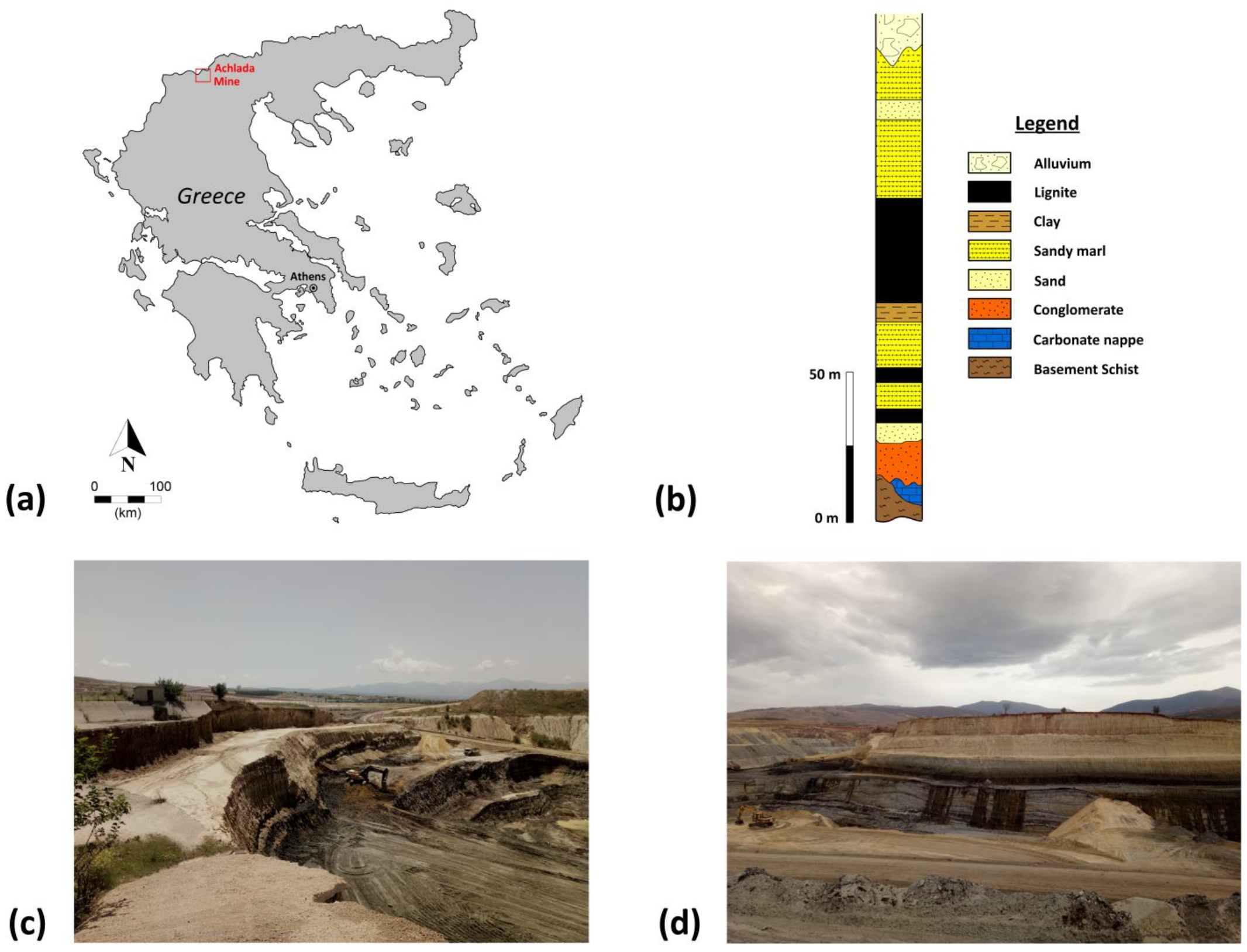
2. Site Location, Regional Geology, Hydrogeology, and Mine Conditions

This case study relates to the stability analysis of a slope in Achlada open pit mine (Northern Greece) (Figure 1). The mining development site extends into the Florina Basin that comprises Paleozoic schists (bedrock), Mesozoic carbonate rocks, Neogene formations, and Alluvium sediments.
The Neogene formations that fill the Florina Basin overlay the basement (composed of Paleozoic schists [28,29]) and include three lithostratigraphic units:
(i)
The lowest consists of conglomerates with a maximum thickness of about 200 m. A transitional passage into marls, sandy marls, sands, clays, and thin lignite horizons is present upwards.
(ii)
The middle unit comprises a clayey formation with thick lignite beds, marls, sandy marls, and sands. Conglomerates and marly limestone lenses are also occasionally present [30].
(iii)
The upper unit includes alternations in clays, marls, marly breccia, and sandy conglomerates.
Quaternary sedimentation is represented by lacustrine and terrestrial sediments such as sandy clays, clay marls, sandy marls, lignite, lateral fans, and alluvial deposits [28,31].
Different hydrogeologic parameters characterize the geological formations throughout the study area. In particular, the alluvial deposits with various grain compositions and cross-bedding patterns present different hydrogeological features from one place to another. Their hydraulic conductivity value is estimated to fall within the range of 10−4 to 10−7 m/s.
In contrast, the Neogene deposits have a lower permeability (10−8 m/s) due to their lithological composition. It is noted that low-yield aquifers are present in the Pleistocene conglomerates and sandstone formations, as presented in Figure 2.
In the mine area, the prevailing geological composition includes Neogene formations. The presence of alternating layers of marl and marly sandstone characterizes them. The composition of the marl layers ranges from clay silt to silt, with varying proportions of sand. The thickness of layers ranges from 10 m to 30 m, with recorded intercalations of lignite/xylite ranging from 10 cm to 2 m in thickness. The marly sandstone with low cohesion comprises compacted silty sand particles.
Stability analysis was carried out on a slope of Achlada mine (Figure 2) that is considered to be a representative of the ground profile of the site. The slope is composed of alternating sandstone and marl formations. Their properties, summarized in Table 1, were obtained from laboratory testing on samples attained from drilling [32], data present in the technical report for mine design [33,34], and bibliographic references concerning the grain size and structure of the geologic formations [34,35]. As mentioned by Ural and Yuksel [36], detailed geotechnical data often represents a significant risk in slope design. It is worth noting that determining the geotechnical parameters is associated with uncertainties due to problems related to heterogeneity, sampling, and laboratory testing. As a result, the adoption of the geotechnical parameters was treated with caution.

3. Evaluation of Slope Stability

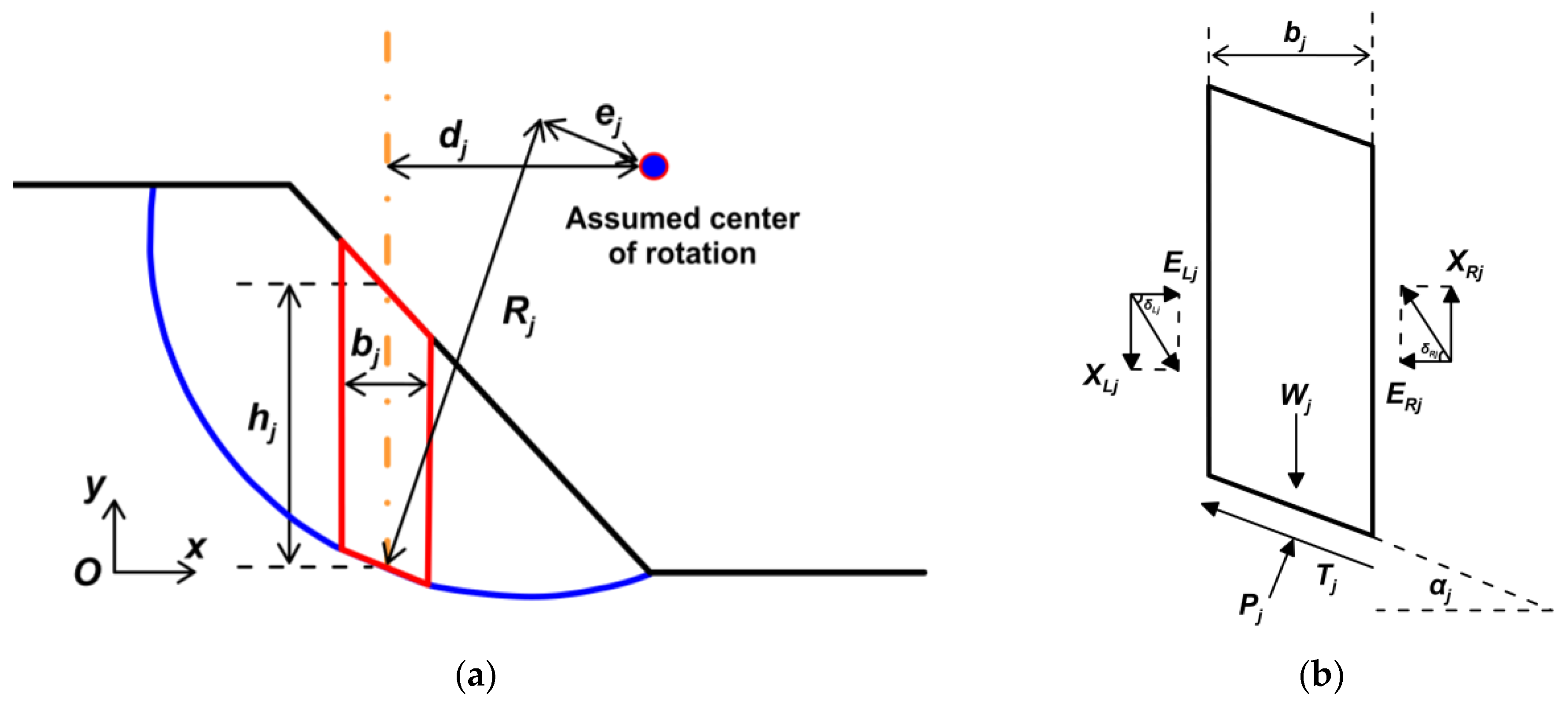
3.1. Limit Equilibrium Methods

The Morgenstern–Price method (M-P) was applied for the slope stability analysis using the GeoSlope software [37]. The M-P method is the most appropriate and comprehensive approach for evaluating the stability of a slope that comprises alternating geological formations.
The slope is divided into n vertical slices (red line), j = 1 ,   2 , n , with thickness b j and height h j , where the forces and moments are analyzed in Figure 3. More specifically, the moments are estimated based on the weight W j , the horizontal distance, of slice’s center of mass (orange dash line) d j from the center of rotation, the normal reaction force P j with the distance e j , and the shear reaction force T j with the distance R j . In Figure 3, the inclination of the jth slice is depicted as α j , while the horizontal and vertical interface forces are depicted as Δ E j = E R j E L j and Δ X j = X R j X L j , respectively.
For the correlation between the horizontal and vertical force, Equation (1) is used [39,40,41].
t a n δ j = Δ X j Δ E j = λ · f x ,
where λ = scale factor, and the assumed function f ( x ) is defined by Equation (2):
f x = s i n μ π · x a b a ν ,
where μ and ν are parameters that determine the shape of the function, and a ,   b are the left and right x coordinates of intersection of the slip surface with the slope profile.
A factor of safety with respect to moment equilibrium ( F S m ) and a second one with respect to horizontal force equilibrium ( F S f ) are estimated by Equation (3) and Equation (4), respectively, considering various shear to normal stress ratios, referred to as lambda ( λ ).
F S m λ = j = 1 n c j · b j c o s α j + P j λ · t a n φ j · R j j = 1 n W j · d j P j λ · e j ,
F S f λ = j = 1 n c j · b j c o s 2 α j + P j λ c o s α j · t a n φ j · R j j = 1 n W j Δ X j λ · t a n φ j ,
where c j and φ j are cohesion and internal friction parameters, while normal interaction forces in the slice base P j λ and shear interaction forces with the j 1 th and j + 1 th slices Δ X j λ are expressed as a function of the scale factor of Equation (1).
An iterative process continues until F S m and F S f are within a specified tolerance limit [42]. Then, the solution is considered to have converged to the safety factor.
The results obtained from the LEM stability analysis and the GeoSlope software (2019 version) [37] are presented in Figure 4 (number of slices: 50). Most of the critical failure surfaces are circular, passing through the slope toe (Figure 4), and they exhibit similar safety factors. Given the near proximity of safety factors concerning the critical failure surfaces, it is highly likely that many surfaces may experience failure, and they should be considered while designing slope. The global minimum factor of safety (FS) is 1.510, but a local minimum FS of 1.389 is also found in the upper part of the slope (Figure 4). The presence of a local minima makes it difficult to locate the critical slip surface.
Field research and engineering judgment are valuable tools to set the potential failure surface and obtain the desired results. The water table is represented by dashed blue line. The inverted triangle indicates the depth at which the water table is met.

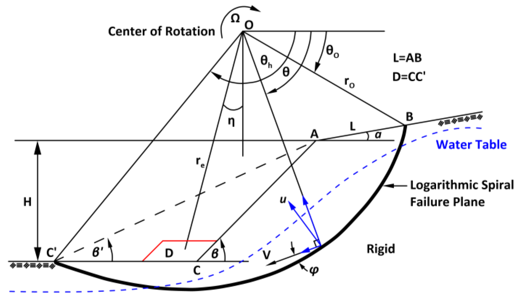
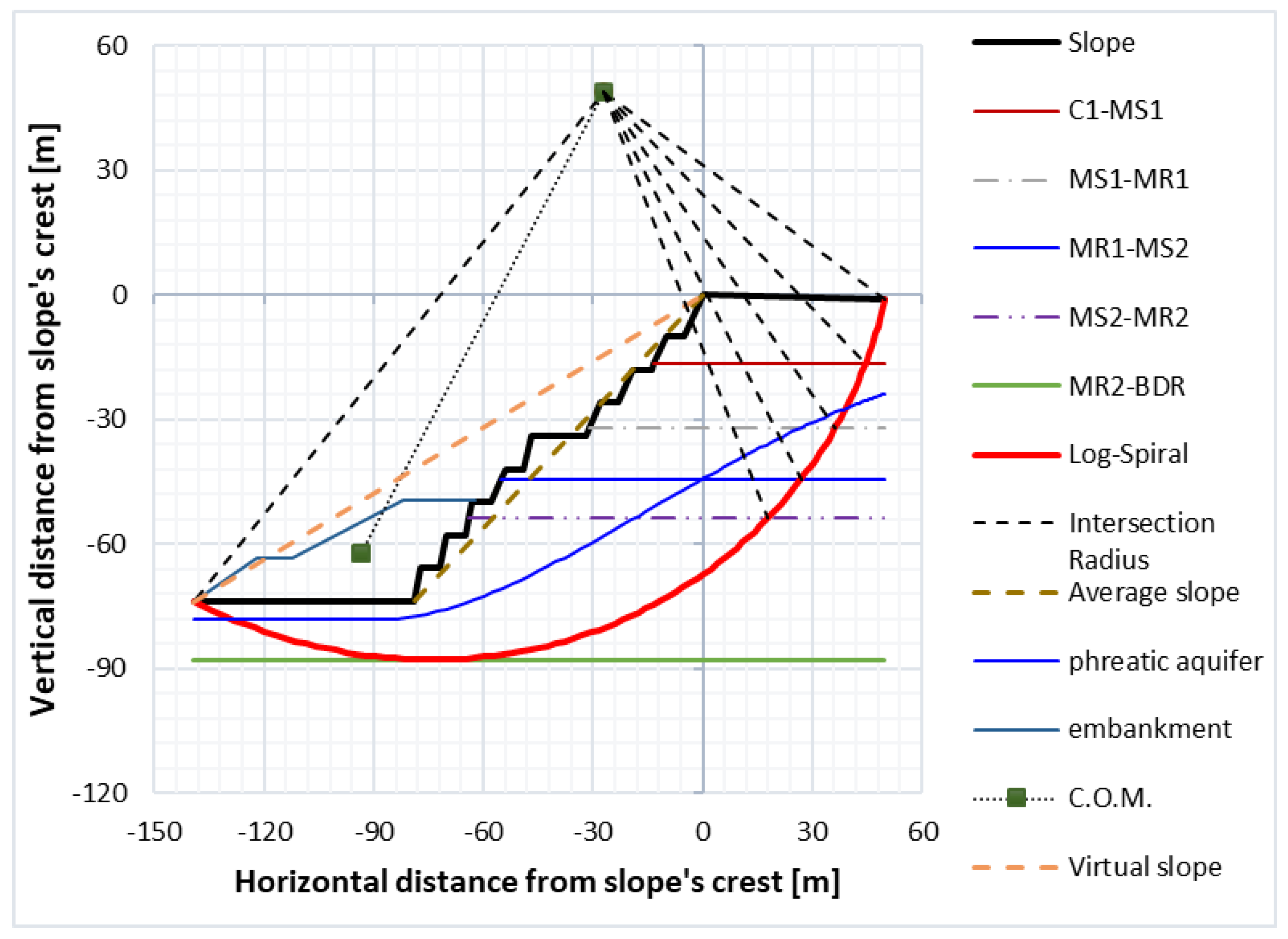
3.2. Limit Analysis and Upper-Bound Theorem

The limit analysis (LA) method, based on the upper bound theorem of plasticity, was applied for the slope stability assessment. Although less known, LA has been used successfully in the recent decades for slope stability analysis [42,43,44,45]. By defining the kinematic mechanism of the slope and calculating the produced work during sliding, the consumed energy is estimated on the basis of the ideal plasticity theory and the Mohr–Coulomb (M-C) criterion. The upper-bound solution (that implies collapse) is obtained from the energy balance [46]. The work associated with plastic deformation is estimated by multiplying the slip surface with cohesion and the displacement (or the velocity) of the mass in the direction of sliding. The rotational mechanism solution is derived using the logarithmic spiral, a natural function with the most typical case being the Nautilus shell and the formation of typhoons [47]. In slope failure (Figure 5), this mechanism is related to the internal friction angle of soil formation according to Equation (5):
r = r 0 · e θ θ 0 · t a n φ ,
where r 0 is the radius of angle θ 0 , and r is the radius of angle θ (Figure 5).
The pore water pressure u estimated from phreatic aquifer surface (blue line) applied to the slip surface (red line), is separated into radial u r and tangential u θ components; only the latter produces work (Figure 5).
The estimation of the work generated by the rotating moment of the slope involves the separation of the mass into distinct components (Figure 5). These components include the region ( F 1 ) located above the logarithmic spiral arc O A C , as well as the portions ( F 2 ) and ( F 3 ) referring to the triangles O A B and O B C ,   r e s p e c t i v e l y . The respective dimensionless works f1, f2, and f3 are estimated using Equation (6), Equation (7), and Equation (8), respectively [46].
f 1 = F 1 γ · r 0 3 · ω = θ 0 θ h 2 3 · r r 0 · c o s θ · 1 2 · r 2 r 0 2 d θ = 3 · t a n φ · c o s θ h + s i n θ h · r h 3 3 · t a n φ · c o s θ 0 + s i n θ 0 · r 0 3 3 · r 0 3 · 1 + 9 · t a n 2 φ ,
f 2 = F 2 γ · r 0 3 · ω = 1 3 · 2 · c o s θ 0 L r 0 · c o s α · 1 2 · L r 0 · s i n θ 0 + α ,
f 3 = F 3 γ · r 0 3 · ω = 1 3 · c o s θ 0 L r 0 · c o s α + r h r 0 · c o s θ h · 1 2 · r h r 0 · h r 0 · s i n θ h + β s i n β ,
where ω is the angular velocity. The terms r 0 and r h denote the log-spiral radii and α and β the angles, shown in Figure 5.
The produced work during sliding C , consumed on the A C surface (Figure 5), is calculated using Equation (9) [46]:
C = θ 0 θ h c · V · c o s φ · r c o s φ d θ = c · r h 2 r 0 2 · ω 2 · t a n φ ,
where c is the cohesion, and φ is the friction angle of the soil formation, and V is the radial speed of the mass.
The log-spiral trajectory is defined on the basis of angles θ 0 and θ h (Figure 5) and Equations (10) and (11).
h r 0 = s i n β s i n β α · r h · s i n θ h + a r 0 · s i n θ 0 + a r 0 ,
L r 0 = s i n θ h θ 0 s i n θ h + α s i n θ h + β s i n β α · r h r 0 s i n θ 0 + α s i n θ h + α ,
The terms θ 0 , and θ h denote the log-spiral angles from the horizontal axis in a clockwise direction as depicted in Figure 5.
The critical slope height ( h c r ) is calculated with Equation (13). It is derived using the energy balance equation, i.e., Equation (12), substituting the ratio of h / r 0 with the value defined by Equation (11).
C = F 1 F 2 F 3 ,
h c r = c γ · s i n β 2 · s i n β α · t a n φ · e 2 · θ h θ 0 · t a n φ 1 f 1 f 2 f 3 · e θ h θ 0 · t a n φ · s i n θ h + a s i n θ 0 + a ,
It is important to note that the procedure described above is suitable for slopes that consist of a single geomaterial layer [46]. In order to implement the aforementioned methodology for multi-layered slopes, it is recommended to utilize the equivalent properties φ ¯ ,   c ¯ , and γ ¯ of the soil formations. In detail, the equivalent internal friction angle φ ¯ is calculated using a weighted average with a log-spiral arc length determined according to Equation (14):
t a n φ ¯ = i = 1 n t a n φ i · θ i 1 θ i e θ θ 0 · t a n φ ¯ d θ θ 0 θ h e θ θ 0 · t a n φ ¯ d θ = i = 1 n t a n φ i · e θ i θ 0 · t a n φ ¯ e θ i 1 θ 0 · t a n φ ¯ e θ h θ 0 · t a n φ ¯ 1 ,
The ultimate value is determined using an iterative procedure, commencing from the friction angle value of the thicker layer. Similarly, the equivalent cohesion c ¯ and equivalent unit weight γ ¯ are calculated using Equation (15) and Equation (16), respectively, to obtain the respective consumed and produced works.
c ¯ = i = 1 n c i · θ i 1 θ i e 2 · θ θ 0 · t a n φ ¯ d θ θ 0 θ h e 2 · θ θ 0 · t a n φ ¯ d θ = i = 1 n c i · e 2 · θ i θ 0 · t a n φ ¯ e 2 · θ i 1 θ 0 · t a n φ ¯ e 2 · θ h θ 0 · t a n φ ¯ 1 ,
γ ¯ = i = 1 n γ i · f 1 i 1 f 2 i 1 f 3 i 1 f 1 i + f 2 i + f 3 i f 1 f 2 f 3 ,
where θ 0 is the log-spiral angle of top surface,
θ i is the log-spiral angle of intersection between i and i + 1 soil layers,
θ n = θ h is the log-spiral angle of slope toe, and
f 1 i , f 2 i , and f 3 i are defined from Equations (6)–(8) and Equations (10) and (11) by substituting θ 0 = θ i and r 0 = r i .
The strength reduction approach [44] is employed to reduce the shear strength parameters c d = c ¯ / F and t a n φ d = t a n φ ¯ / F by a factor of F until failure. This reduction leads the slope closer to the critical limit equilibrium condition; the critical height ( h c r ) is equivalent to the actual height ( h c r = h ), while the F parameter represents an estimate of the safety factor ( F S = F ).
In the case of presence of groundwater, the generated work is estimated by considering its velocity component as depicted in Figure 5 and Figure 6. The water column’s height can be estimated as a polynomial function of the angle ( θ ) and the maximum height of water ( h w m a x ) as depicted in Figure 5, according to Equation (17):
U = θ 1 θ 2 γ w · h w θ · s i n φ ¯ · V · r c o s φ ¯ d θ = θ 1 θ 2 γ w · 4 · θ θ 1 · θ 2 θ θ 2 θ 1 2 · h w m a x · t a n φ ¯ · V · r d θ = γ w θ 2 θ 1 2 · h w m a x r 0 · r 0 · { r 1 2 · θ 1 2 + θ 1 + 1 t a n φ ¯ 2 r 2 2 · θ 2 2 + θ 1 + 1 t a n φ ¯ 2 + 2 · θ 1 · θ 2 · r 1 2 r 2 2 θ 1 + θ 2 · r 1 2 · 2 · θ 1 1 t a n φ ¯ r 2 2 · 2 · θ 2 1 t a n φ ¯ } ,
The critical height ( h c r ) is then found using Equation (18), considering the height of water along the sliding surface (Figure 5):
h c r = C · r 0 F 1 F 2 F 3 + U · H r 0 ,
In the most possible scenario, the slip surface goes beneath the slope’s toe, as shown in Figure 6. Its mechanism is equivalent to that shown in Figure 5, with the virtual slope of β angle defined by the line passing through the slope’s crest (point A) and the toe (point C’). The calculations are derived from Equations (11)–(13), considering the angle β instead of β .
Figure 6. Slide mechanism below the slope toe (modified based on [46]). Signs along the toe and crest denote the land surface.
Geosciences 13 00359 g006
Considering the geomorphic characteristics of the study area, the produced work related to the excavation and the formation of the slope is associated with section ACC’ (Figure 6), and it is estimated using Equation (19) [46]:
F 4 = γ · r 0 3 · ω · H r 0 2 · s i n β β 2 · s i n β · s i n β · c o s θ 0 L r 0 · c o s α 1 3 · H r 0 · c o t β + c o t β ,
In addition, the presence of the embankment (D) (Figure 6), results in the consumption of the work due to the introduction of torque that opposes the motion of the slope. The resulting energy can be determined through the utilization of Equation (20):
F 5 = γ e · A e · r e · s i n η · ω ,
where γ e is the unit weight of the embankment, A e is the embankment’s cross-section area, r e is the distance between the center of rotation and the center of mass gravity (C.O.M.), and η the angle formed between the vertical axis and the line passing through the center of rotation and the center of mass.
The critical height in this particular scenario is determined using Equation (21):
h c r r 0 = C F 1 F 2 F 3 F 4 F 5 + U · H r 0 ,
To ensure the attainment of a precise solution, the toe of the slide is considered to extend beyond the embankment. Also, it is considered that the lower portion of the log-spiral ( θ = π / 2 + φ ) comes into contact with or rests against the bedrock formation that is characterized by a high shear strength. Additionally, the slip curve exhibits a consistent increase along the horizontal axis.
For the stability evaluation and definition of the geometry (location and shape) of the critical failure surface, a modified logarithmic spiral method using the upper-bound theorem was applied. Considering the above restrictions and assuming that the hydrostatic stress in the mass equilibrates the pore water pressure, the stability of the multi-layered slope was calculated using the excel worksheet provided in Supplementary Materials (Geoscience_Upper_Bound_Multilayer_Slope.xlsx). The safety factor was estimated equal to F S = 1.472 , and the crucial slip surface depicted in Figure 7 compares well with the slip surface defined from the limit equilibrium method.

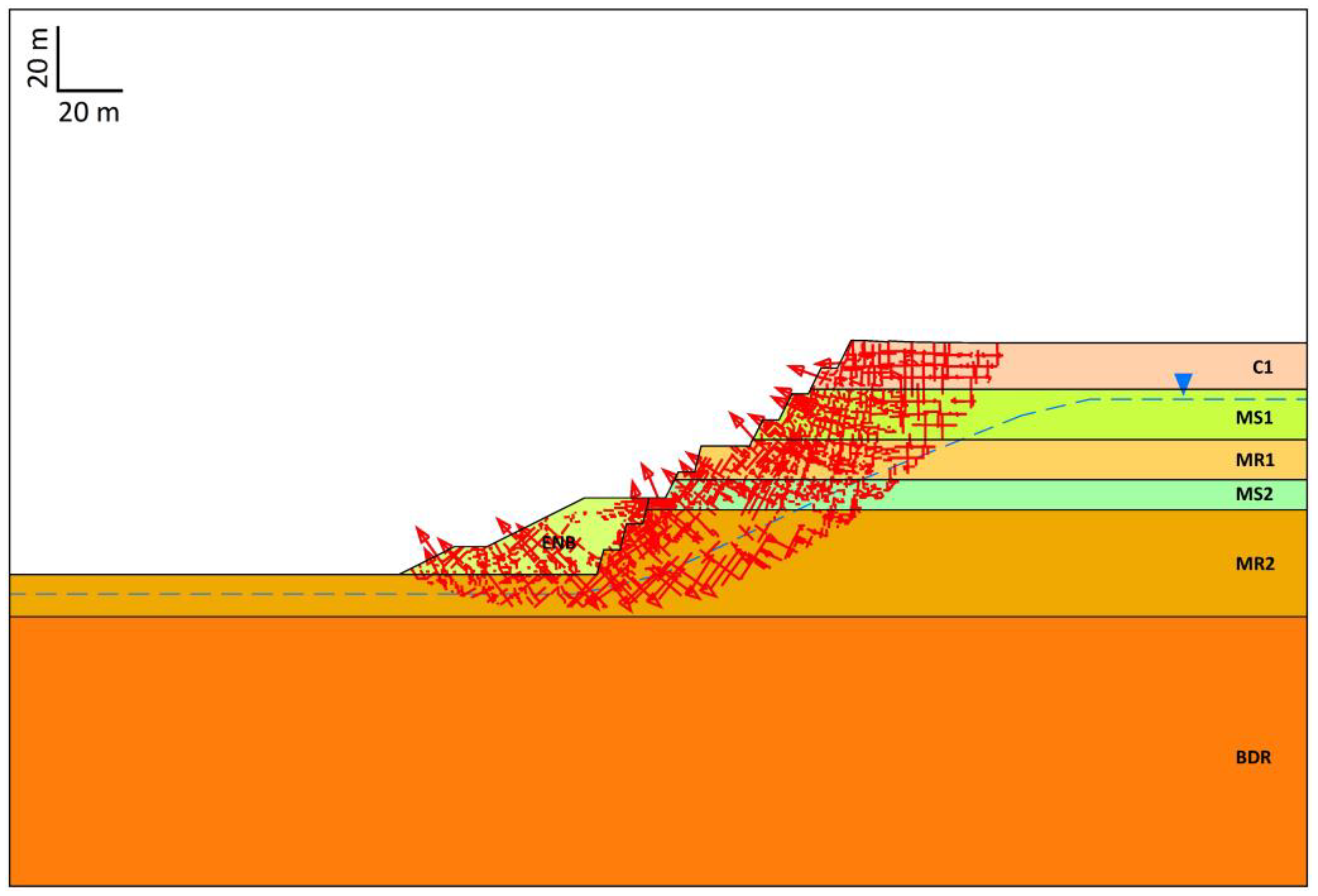
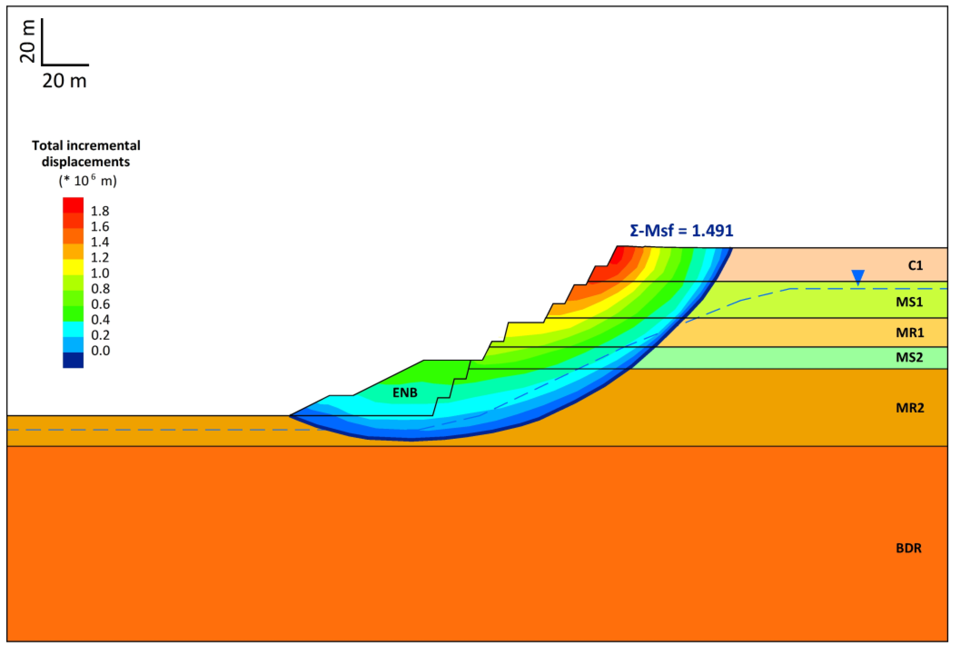
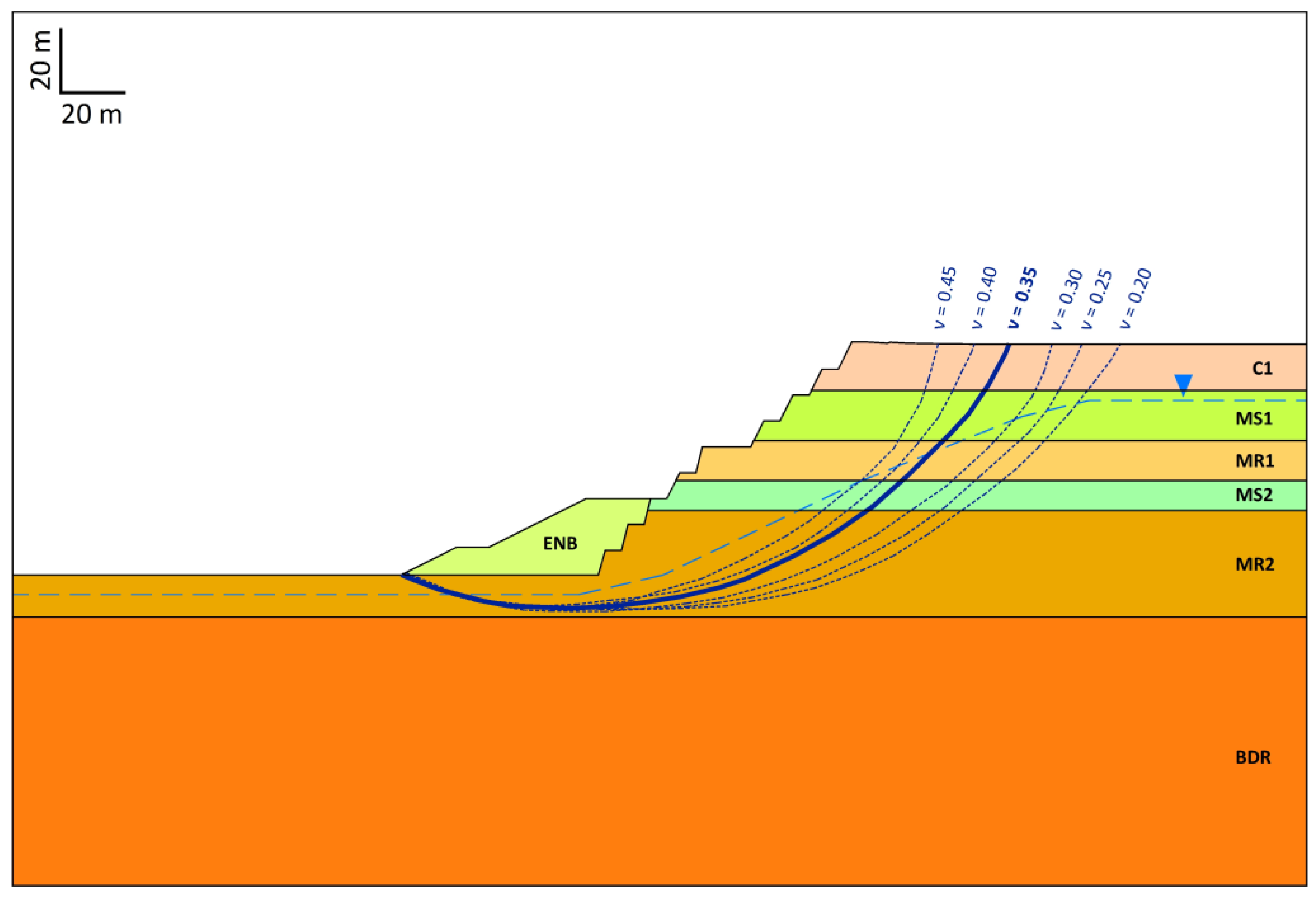
3.3. Finite Element Method

The slope stability analysis was conducted based on the numerical simulation using the Plaxis 8.2 software [48]. The use of finite element methods is a widespread technique in recent years for calculating displacement instabilities in open pit mines [33,34,49,50,51,52]. The numerical analysis was carried out on the cross-section presented in Figure 2. For the numerical simulation, the soil layers were modelled using the relatively simple elastic and perfectly plastic Mohr–Coulomb (M-C) model, which employs the strength parameters ( c ,   φ ), the dilatancy angle ( i ), and the elastic parameters ( E , ν ). The geotechnical parameters for each soil formation modelled in the simulation are presented in Table 1.
The model was designed to extend below the toe and away from the crest of the slope to minimize the effect of the boundary conditions [33,34,49]. A plane strain model with 15-node triangular elements was adopted for the current study. Following the input of the soil parameters, a finite element mesh was created using the Plaxis software; the generated mesh is considered capable of providing a reliable analysis. The vertical boundaries were fixed in the horizontal direction, and the bottom boundary was fixed in both directions, considering that the base of the slope was stiff enough. Pore pressures were generated on the basis of phreatic line defined through measurements in the field. Using the input of the phreatic surface, the water pressure increases linearly with depth according to the specified water weight (hydrostatic). Given the values of permeability coefficients determined through Maag tests (Table 1), and considering the excavation phases and slope formation rate, the analysis was carried out in drained conditions.
Numerical simulation offered the possibility to calculate the displacements, to localize the deformations strains in the mass (Figure 8), and to determine the safety factor according to displacement (Figure 9).
The incremental strains (Figure 8) highlight the limit between the zone where no displacement (zero value) occurs and the zone where displacements (non-null values) occur. The shape of deformation localization in the slope is nearly circular and confirms the shape of the critical failure surface, defined using the LEM method. The critical failure surface intersects the slope and passes through the toe of the slope and along the base of MS2 formation.
The safety factor was found using the c-phi reduction approach according to the Mohr–Coulomb criterion. The method is based on the reduction in the cohesion ( c ) and the tangent of the internal friction angle ( t a n φ ) of the soil until the failure of the slope occurs. It is noted that the analyses were performed using constant Poisson’s ratios ( v ) and Young’s modulus ( E ) of the formations, presented in Table 1, and the value of the safety factor, and it was found to be equal to 1.491 (Figure 9).
As Duncan states in [1], one of the problems with using a constant value of Poisson’s ratio ( v ) is that it is difficult to select a value of ( ν ) logically because its value depends on the stress conditions to which the soil is subjected [1,53]. In order to investigate the effect of Poisson’s ratio and the overall deformation model on the slope stability, different Poisson’s values for the soil formations were considered. The analyses indicate that the results are sensitive to the considered Poisson’s ratios of the soil formations (Figure 10). When the Poisson’s ratio of the soil formations changes, the location of the critical slip surface alters, depending on the situation being analyzed (Figure 10).
In detail, the critical slip surface passes through the toe, and the upper end of the slip surface moves closer to the slope’s crest as the Poisson’s ratio of the soil formations increases. However, this variation does not change significantly due to the small differentiation of the precarious mass and the fixed value of friction angle and cohesion for the soil layers. The solution result was compared with field measurements, and the geometry of the critical surface was verified using the data gathered through monitoring and evaluation studies (Figure 11).

4. Discussion

Limit equilibrium method (LEM) reveals that although most critical slip surfaces have identical values of the safety factor, the geometry of the sliding mass might vary (Figure 4).
This makes it difficult to locate the critical surface using classical optimization methods. Therefore, field observations and engineering judgments considering indicated signs of failure should be evaluated for proper results.
When the location and shape of the critical failure surface are challenging to examine in detail in a multi-layered slope, the usage of the LA (upper-bound analysis) performed using an Excel worksheet may be especially intriguing. This worksheet makes it simple to use the analysis, minimizing the need for familiarization with commercial tools. However, it is noted that the complexity of the geology and the existing aquifer make the solution obtained with the LEM more flexible.
Regarding the FEM method, it represents a powerful tool for slope stability analysis in multi-layered formation, as it allows a consideration of a variety of factors that influence the mobility and highlights sensitive zones that require careful examination. Specifically, the results demonstrate that the proper value of Poisson’s ratio (v) is prerequisite for reliable results as it affects the size and location (geometry) of the critical slip surfaces. In detail, the upper end of the failure surface moves closer to the slope’s crest as the Poisson’s ratio of the soil formation increases. Therefore, quality data concerning the initial conditions and the geotechnical parameters are essential for accurate results.
The comparison between critical slip surfaces obtained using LEM, LA, and FEM shows that all methods provide an almost identical shape and location of the critical slip surface that intersects the slope and passes through the toe. The formation of local minima failure surfaces in the LEM, constitutes a major difference between LEM and FEM. However, the factor of safety for the global slip surface based on the limit analysis and limit equilibrium methods appears to be very close to the value estimated using the finite element method. The safety factor obtained with FEM was underestimated by about 1% compared to that obtained with LEM and overestimated by 1% compared to that obtained with LA.
Furthermore, since the size and shape of the critical slip surface controls the stability, the values of safety factor obtained by each method compare well. Although there are some minor differences, the results are similar, suggesting that the use of either the LEM, LA, or FEM method is generally satisfactory. In view of the differences in the shape and location of the critical slip surface, as well as in those in the obtained values of the safety factor, it is recommended that an engineer should analyze critical slopes using the finite element method (FEM) in combination with the limit equilibrium method (LEM). In any case, project monitoring and engineering judgment are necessary in order to manage the outcomes effectively.

5. Conclusions

The paper performed the stability analysis of a multi-layered slope. The following conclusions were derived from the results. The analysis performed using the LEM (limit equilibrium method) reveals that while the values of safety factors in most critical slip surfaces are similar, the geometry of the precarious mass may differ. This makes it difficult to locate the critical surface.
  • The solution proposed for the LA (limit analysis) in multi-layered slopes constitutes an innovative and easy assessment of the safety factor.
  • FEM (finite element method) represents a powerful tool for slope stability analysis in multi-layered formations, provided that quality data concerning the initial conditions and the geotechnical parameters are available. The results indicate that a proper value of Poisson’s ratio (v) is a prerequisite for obtaining reliable results as it affects the size and location (geometry) of the critical slip surfaces.
  • The formation of local minima failure surfaces in the LEM is referred to as a major difference between the LEM and the FEM, and the study demonstrates that the implementation of FEM combined with LEM or LA provides the most appropriate tool to analyze the slope stability in a multi-layered formation.

Supplementary Materials

The following supporting information can be downloaded at: https://www.mdpi.com/article/10.3390/geosciences13120359/s1. The multi-layered slope stability obtained using limit analysis is presented in the excel worksheet Geoscience_Upper_Bound_Multilayer_Slope.xlsx.

Author Contributions

Conceptualization, E.S.; methodology, E.S. and G.X.; software, D.V. and I.L.; validation, E.S., G.X., I.L. and G.B.; formal analysis, E.S. and G.X.; data curation, D.V. and G.B.; supervision, E.S. All authors have read and agreed to the published version of the manuscript.

Funding

This research received no external funding.

Acknowledgments

The authors wish to thank the Achlada Mine Corporation for providing unpublished information regarding the kinetic behavior of the slope.

Conflicts of Interest

The authors declare no conflict of interest.

References

  1. Duncan, J.M. State Of-the-Art Stability and Deformation Analysis. J. Geotech. Eng. ASCE 1996, 122, 557–597. [Google Scholar]
  2. Fredlund, D.G.; Krahn, J. Comparison of Slope Stability Methods of Analysis. Can. Geotech. J. 1977, 14, 429–439. [Google Scholar] [CrossRef]
  3. Fredlund, D.G.; Krahn, J.; Pufahl, D.E. The Relationship between Limit Equilibrium Slope Stability Methods. Soil mechanics and foundation engineering. In Proceedings of the 10th International Conference, Stockholm, Sweden, 5–19 June 1981; Volume 3. [Google Scholar] [CrossRef]
  4. Fang, H.-Y.; Daniels, J.L. Introductory Geotechnical Engineering: An Environmental Perspective; CRC Press: London, UK, 2017; ISBN 9781315274959. [Google Scholar]
  5. Kim, J.; Salgado, R.; Lee, J. Stability Analysis of Complex Soil Slopes Using Limit Analysis. J. Geotech. Geoenviron. Eng. 2002, 128, 546–557. [Google Scholar] [CrossRef]
  6. Jiang, G.L.; Magnan, J.P. Stability Analysis of Embankments: Comparison of Limit Analysis with Methods of Slices. Geotechnique 1997, 47, 857–872. [Google Scholar]
  7. Chuang, P.H. Stability Analysis in Geomechanics by Linear Programming. II: Application. J. Geotech. Eng. 1992, 118, 1716–1726. [Google Scholar] [CrossRef]
  8. Cheng, Y.M.; Lansivaara, T.; Wei, W.B. Two-Dimensional Slope Stability Analysis by Limit Equilibrium and Strength Reduction Methods. Comput. Geotech. 2007, 34, 137–150. [Google Scholar] [CrossRef]
  9. Strang, G.; Fix, J. An Analysis of the Finite Element Method; Prentice-Hall: Englewood Cliffs, NJ, USA, 1973. [Google Scholar]
  10. Hughes, T. Linear Static and Dynamic Finite Element Analysis. In The Finite Element Method; Dover Publications, Inc.: New York, NY, USA, 1987; Volume 65. [Google Scholar]
  11. Zienkiewicz, O.C.; Taylor, R.L. The Finite Element Method; McGraw-Hill: New York, NY, USA, 1989. [Google Scholar]
  12. Clough, R.W.; Woodward, R.J. Analysis of Embankment Stresses and Deformations. J. Soil Mech. Found. Div. 1967, 93, 529–549. [Google Scholar] [CrossRef]
  13. Hammouri, N.A.; Husein Malkawi, A.I.; Yamin, M.M.A. Stability Analysis of Slopes Using the Finite Element Method and Limiting Equilibrium Approach. Bull. Eng. Geol. Environ. 2008, 67, 471–478. [Google Scholar] [CrossRef]
  14. Wright, S.G.; Kulhawy, F.H.; Duncan, J.M. Accuracy of Equilibrium Slope Stability Analysis. J. Soil Mech. Found. Div. 1973, 99, 783–791. [Google Scholar] [CrossRef]
  15. Huang, S.L.; Yamasaki, K. Slope Failure Analysis Using Local Minimum Factor-of-Safety Approach. J. Geotech. Eng. 1993, 119, 1974–1989. [Google Scholar] [CrossRef]
  16. Zienkiewicz, O.C.; Humpheson, C.; Lewis, R.W. Associated and Non-Associated Visco-Plasticity and Plasticity in Soil Mechanics. Géotechnique 1975, 25, 671–689. [Google Scholar] [CrossRef]
  17. Ugai, K. A Method of Calculation of Total Safety Factor of Slope by Elasto-Plastic FEM. Soils Found. 1989, 29, 190–195. [Google Scholar] [CrossRef] [PubMed]
  18. Matsui, T.; San, K.-C. Finite Element Slope Stability Analysis by Shear Strength Reduction Technique. Soils Found. 1992, 32, 59–70. [Google Scholar] [CrossRef]
  19. Ugai, K.; Leshchinsky, D. Three-Dimensional Limit Equilibrium and Finite Element Analyses: A Comparison of Results. Soils Found. 1995, 35, 1–7. [Google Scholar] [CrossRef]
  20. Dawson, E.M.; Roth, W.H.; Drescher, A. Slope Stability Analysis by Strength Reduction. Géotechnique 1999, 49, 835–840. [Google Scholar] [CrossRef]
  21. Manzari, M.T.; Nour, M.A. Significance of Soil Dilatancy in Slope Stability Analysis. J. Geotech. Geoenviron. Eng. 2000, 126, 75–80. [Google Scholar] [CrossRef]
  22. Chang, Y.; Huang, T. Slope Stability Analysis Using Strength Reduction Technique. J. Chin. Inst. Eng. 2005, 28, 231–240. [Google Scholar] [CrossRef]
  23. Liu, F. Stability Analysis of Geotechnical Slope Based on Strength Reduction Method. Geotech. Geol. Eng. 2020, 38, 3653–3665. [Google Scholar] [CrossRef]
  24. Griffiths, D.V.; Lane, P.A. Slope Stability Analysis by Finite Elements. Géotechnique 1999, 49, 387–403. [Google Scholar] [CrossRef]
  25. Song, L.; Yu, X.; Xu, B.; Pang, R.; Zhang, Z. 3D Slope Reliability Analysis Based on the Intelligent Response Surface Methodology. Bull. Eng. Geol. Environ. 2021, 80, 735–749. [Google Scholar] [CrossRef]
  26. Zheng, H.; Liu, D.F.; Li, C.G. Slope Stability Analysis Based on Elasto-Plastic Finite Element Method. Int. J. Numer. Methods Eng. 2005, 64, 1871–1888. [Google Scholar] [CrossRef]
  27. Zaki, A. Slope Stability Analysis Overview. Ph.D. Thesis, University of Toronto, Toronto, ON, Canada, 1999. [Google Scholar]
  28. Pavlides, S.B.; Mountrakis, D.M. Extensional Tectonics of Northwestern Macedonia, Greece, since the Late Miocene. J. Struct. Geol. 1987, 9, 385–392. [Google Scholar] [CrossRef]
  29. Oikonomopoulos, I.K.; Perraki, M.; Tougiannidis, N.; Perraki, T.; Kasper, H.U.; Gurk, M. Clays from Neogene Achlada Lignite Deposits in Florina Basin (Western Macedonia, N. Greece): A Prospective Resource for the Ceramics Industry. Appl. Clay Sci. 2015, 103, 1–9. [Google Scholar] [CrossRef]
  30. Koukouzas, N.; Ward, C.R.; Li, Z. Mineralogy of Lignites and Associated Strata in the Mavropigi Field of the Ptolemais Basin, Northern Greece. Int. J. Coal. Geol. 2010, 81, 182–190. [Google Scholar] [CrossRef]
  31. Metaxas, A.; Karageorgiou, D.E.; Varvarousis, G.; Kotis, T.; Ploumidis, M.; Papanikolaou, G. Geological Evolution—Stratigraphy of Florina, Ptolemaida, Kozani and Saradaporo Graben. Bull. Geol. Soc. Greece 2018, 40, 161–172. [Google Scholar] [CrossRef]
  32. Geoter, G.; Didaskalou, S.P. Results of Laboratory Tests on Selected Samples of Boreholes NG2/14, NG11/14, NG12/14; Report of geotechnical investigation in Achlada Mine; 2014, unpublished data. (In Greek).
  33. Steiakakis, E.; Agioutantis, Z.; Monopolis, D. An Investigation of the Kinetic Behavior of a Deep Excavation at an Open Pit Mine Using Finite Elements Analysis. In Proceedings of the AMIREG, Chania, Greece, 7–9 June 2004; pp. 51–56. [Google Scholar]
  34. Steiakakis, E.; Kavouridis, K.; Monopolis, D. Large Scale Failure of the External Waste Dump at the “South Field” Lignite Mine, Northern Greece. Eng. Geol. 2009, 104, 269–279. [Google Scholar] [CrossRef]
  35. Arvanitidis, C.; Steiakakis, E.; Agioutantis, Z. Peak Friction Angle of Soils as a Function of Grain Size. Geotech. Geol. Eng. 2019, 37, 1155–1167. [Google Scholar] [CrossRef]
  36. Ural, S.; Yuksel, F. Geotechnical Characterization of Lignite-Bearing Horizons in the Afsin–Elbistan Lignite Basin, SE Turkey. Eng. Geol. 2004, 75, 129–146. [Google Scholar] [CrossRef]
  37. Geostudio 2019 R2; Geoslope International Ltd.: Calgary, AB, Canada, 2019.
  38. Zhang, J.; Li, J. A Comparative Study between Infinite Slope Model and Bishop’s Method for the Shallow Slope Stability Evaluation. Eur. J. Environ. Civ. Eng. 2021, 25, 1503–1520. [Google Scholar] [CrossRef]
  39. Ouyang, W.; Liu, S.-W.; Yang, Y. An Improved Morgenstern-Price Method Using Gaussian Quadrature. Comput. Geotech. 2022, 148, 104754. [Google Scholar] [CrossRef]
  40. Morgenstern, N.R.; Price, V.E. The Analysis of the Stability of General Slip Surfaces. Geotechnique 1965, 15, 79–93. [Google Scholar] [CrossRef]
  41. Atashband, S. Evaluate Reliability of Morgenstern–Price Method in Vertical Excavations. In Numerical Methods for Reliability and Safety Assessment; Springer International Publishing: Cham, Switzerland, 2015; pp. 529–547. [Google Scholar]
  42. Zhu, D.Y.; Lee, C.F.; Qian, Q.H.; Chen, G.R. A Concise Algorithm for Computing the Factor of Safety Using the Morgenstern– Price Method. Can. Geotech. J. 2005, 42, 272–278. [Google Scholar] [CrossRef]
  43. Michalowski, R.L.; Nadukuru, S.S. Three-Dimensional Limit Analysis of Slopes with Pore Pressure. J. Geotech. Geoenviron. Eng. 2013, 139, 1604–1610. [Google Scholar] [CrossRef]
  44. Zhao, L.; Qiao, N.; Zhao, Z.; Zuo, S.; Wang, X. Comparative Study of Material Point Method and Upper Bound Limit Analysis in Slope Stability Analysis. Transp. Saf. Environ. 2020, 2, 44–57. [Google Scholar] [CrossRef]
  45. Gao, Y.; Song, W.; Zhang, F.; Qin, H. Limit Analysis of Slopes with Cracks: Comparisons of Results. Eng. Geol. 2015, 188, 97–100. [Google Scholar] [CrossRef]
  46. Chen, W.F. Limit Analysis and Soil Plasticity: Developments in Geotechnical Engineering 7; Elsevier: Amsterdam, The Netherlands, 1975. [Google Scholar]
  47. Niu, H.; Dong, G.; Ma, X.; Ma, Y. An Analytical Model of a Typhoon Wind Field Based on Spiral Trajectory. Proc. Inst. Mech. Eng. Part M J. Eng. Marit. Environ. 2017, 231, 818–827. [Google Scholar] [CrossRef]
  48. Plaxis, B.V. Plaxis Finite Element Code for Soil and Rock Analyses; Version 8; RBJ Brinkgreve: Delft, The Netherlands, 2004. [Google Scholar]
  49. Steiakakis, E.; Agioutantis, Z. A Kinetic Behavior Model at a Surface Lignite Mine, Based on Geotechnical Investigation. Simul. Model Pract. Theory 2010, 18, 558–573. [Google Scholar] [CrossRef]
  50. Dyson, A.P.; Tolooiyan, A. Prediction and Classification for Finite Element Slope Stability Analysis by Random Field Comparison. Comput. Geotech. 2019, 109, 117–129. [Google Scholar] [CrossRef]
  51. Liu, S.; Su, Z.; Li, M.; Shao, L. Slope Stability Analysis Using Elastic Finite Element Stress Fields. Eng. Geol. 2020, 273, 105673. [Google Scholar] [CrossRef]
  52. Gupta, V.; Bhasin, R.K.; Kaynia, A.M.; Kumar, V.; Saini, A.S.; Tandon, R.S.; Pabst, T. Finite Element Analysis of Failed Slope by Shear Strength Reduction Technique: A Case Study for Surabhi Resort Landslide, Mussoorie Township, Garhwal Himalaya. Geomat. Nat. Hazards Risk 2016, 7, 1753. [Google Scholar] [CrossRef]
  53. Ping, J.; Mengsu, Z. Elastic Parameters Adjusted in Soil Slope Stability and Displacement Analysis. Appl. Mech. Mater. 2013, 303, 2889–2892. [Google Scholar]
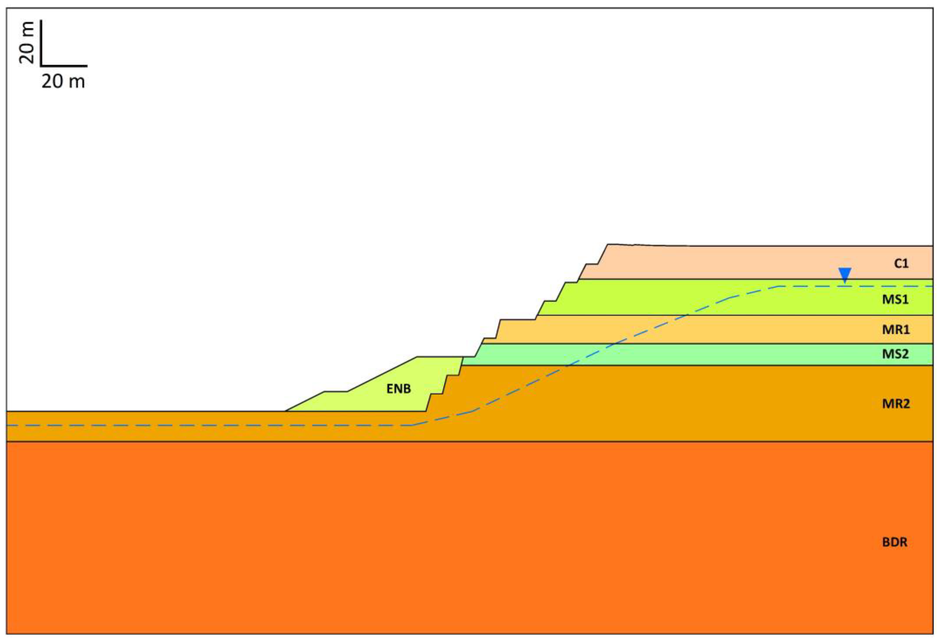
Figure 1. (a) Location of Achlada mine, (b) lithological column of the Florina Basin (created with base [28]), and (c,d) photos of the mine.
Geosciences 13 00359 g001
Figure 2. Slope geometry. C1: upper silty/marly clay zone, MS1: upper sand/pebble sandstone zone, MR1: intermediate silt/silt loam zone with the presence of xylite interbeds, MS2: lower sand/marly sandstone zone, MR2: lower silt/silt loam zone with the systematic presence of xylite, BDR: underlying marl formation, and ENB: counterweight. The upside-down triangle and the blue dashed line indicate the water table.
Geosciences 13 00359 g002
Figure 3. Method of slices: (a) rotational mechanism analysis and (b) forces acting on a slice (modified based on [38]).
Geosciences 13 00359 g003
Figure 4. Global and local minima failure surfaces determined using LEM. The upside-down triangle and the blue dashed line indicate the water table.
Geosciences 13 00359 g004
Figure 5. Log-spiral kinematical mechanism (modified based on [46]). The blue line indicates the water table and the red lines determine the geometry of failure mechanism.
Geosciences 13 00359 g005
Figure 7. Slip surface with the minimum safety factor for the multi-layered slope with LA.
Geosciences 13 00359 g007
Figure 8. Incremental strains (FEM). The upside-down triangle and the blue dashed line indicate the water table.
Geosciences 13 00359 g008
Figure 9. Critical slip surface determination based on the total incremental displacements and the c-phi reduction technique (FEM). The upside-down triangle and the blue dashed line indicate the water table.
Geosciences 13 00359 g009
Figure 10. Slip surface comparison with changes in Poisson’s ratio ( v ) for the soil layers using FEM. The upside-down triangle and the blue dashed line indicate the water table.
Geosciences 13 00359 g010
Figure 11. (a) Comparison of critical slip surface based on LEM, LA, and FEM, respectively. The water table is represented by dashed blue line. The upside-down triangle and the blue dashed line indicate the water table. VI/3: inclinometer location. (b) Monitoring data registered by the inclinometer are shown on the right side of the figure.
Geosciences 13 00359 g011
Table 1. Geotechnical parameters of sedimentary formations. Soil properties for Figure 2.
Soil NameUnit
Weight (kN/m3)
Saturated Unit
Weight
(kN/m3)
Cohesion
(kPa)
Friction
Angle
(°)
Elastic
Modulus
(MPa)
Poisson
Ratio
Permeability Coefficient
(m/s)
C120213522250.281 × 10−7
MS122231039600.301 × 10−6
MR120216526400.281 × 10−7
MS222231241700.301 × 10−6
MR220215025350.351 × 10−7
BDR1819100351000.301 × 10−8
ENB2021332500.251 × 10−6
Disclaimer/Publisher’s Note: The statements, opinions and data contained in all publications are solely those of the individual author(s) and contributor(s) and not of MDPI and/or the editor(s). MDPI and/or the editor(s) disclaim responsibility for any injury to people or property resulting from any ideas, methods, instructions or products referred to in the content.

