Characteristic Magnitude and Spatiotemporal Relationships of Aftershocks and Background Earthquakes

Abstract

Aftershocks, background earthquakes, and their spatiotemporal parameters have been studied for decades for the purpose of hazard assessment and forecasting. Methods for determining these parameters or seismic attributes are becoming increasingly sophisticated and varied; some optimize the results to fit observations using trial and error, while others do the same by giving prescriptions for a limited region. Here, we propose a method that is potentially useful in general hazard assessment and forecasting applications. We categorized the earthquakes into two groups, aftershocks (triggered events) and background earthquakes, by introducing the network distance, i.e., the shortest distance between two events of equal magnitude within a modified interevent time, into the k-means clustering, which couples the modified interevent time and magnitude hierarchically. Our results show a bimodal distribution consisting of a power law at shorter network distances and a lognormal distribution at longer network distances, implying that earthquakes of magnitudes larger than the characteristic magnitude, found to be 4.5 for Taiwan and 4.3 for California, may be only weakly linked to other same magnitude earthquakes and hence are hard to be triggered even by events of larger size.

1. Introduction

A background earthquake is typically one that is not triggered by another. Alternatively, in seismic hazard assessment, the phrase may refer to an earthquake not associated with a known fault. Resulting from tectonic loading, the characteristics of background earthquakes reflect the associated fault physics. As such, background seismicity rate changes are useful for detecting changes in earthquake source systems [1,2,3,4].

Aftershocks constitute another vital component in the earthquake catalog. Aftershocks have been found to be triggered by increasing static stress induced by a mainshock [5,6,7,8] or to be explained by dynamic stress [9,10,11,12]. Those caused by a change in static or dynamic stress usually form a sequence of events occurring near the mainshock in space and time and hence can be considered triggered events. Aftershocks are typically removed from the earthquake catalog for the purpose of forecasting large events, because they would otherwise bias the statistics of background earthquakes.

The mechanics of background earthquakes and triggered earthquakes are characterized by different space–time properties. Triggered earthquakes are typically defined as events occurring within a specified time interval following a mainshock and within a specified radius surrounding a mainshock [13,14,15,16]. The spatial and temporal parameters associated with triggered earthquakes can be determined by the magnitude of the mainshock [13,14] or by an optimized parameter consisting of such parameters [15,16].

However, how to determine mainshocks (or characteristic earthquakes) and verify their spatial and temporal parameters remain unclear. Most branching point process models for earthquake simulation classify seismicity into the two categories of background and triggered earthquakes, and they assume a space–time Poisson process (either stationary or nonstationary and either homogeneous or nonhomogeneous) for background earthquakes [17,18,19,20,21,22,23]. In these models, the intensity function of the background earthquake as a function of space (but not of time) is determined first, and then, the probability density function of triggered earthquakes is optimized according to the location and magnitude of the background earthquake. In other words, a study region and the background earthquakes taking place inside is determined first. As such, background earthquakes are regarded as individual mainshocks followed by clusters of triggered earthquakes.

Statistical models for determining earthquake occurrence probability usually calculate the hazard potential via time series of conditional intensity at each grid point in a study region. However, the conditional intensity can be calculated with different parametric constraints and varies with model definition. For example, the seismicity rate represents a typical conditional intensity and depends on the unit time, area (radius or grid size), and magnitude interval under consideration [24,25,26,27,28,29].

In search of physics-based parameters that can be applied in statistical models, we investigated the spatiotemporal relationships of seismicity and distinguished the background earthquakes and aftershocks using a bimodal model. The model was built based on the distance function of the interevent time, the so-called network distance, so that no conditions and parameters are presumed and that the parameters are self-constrained.

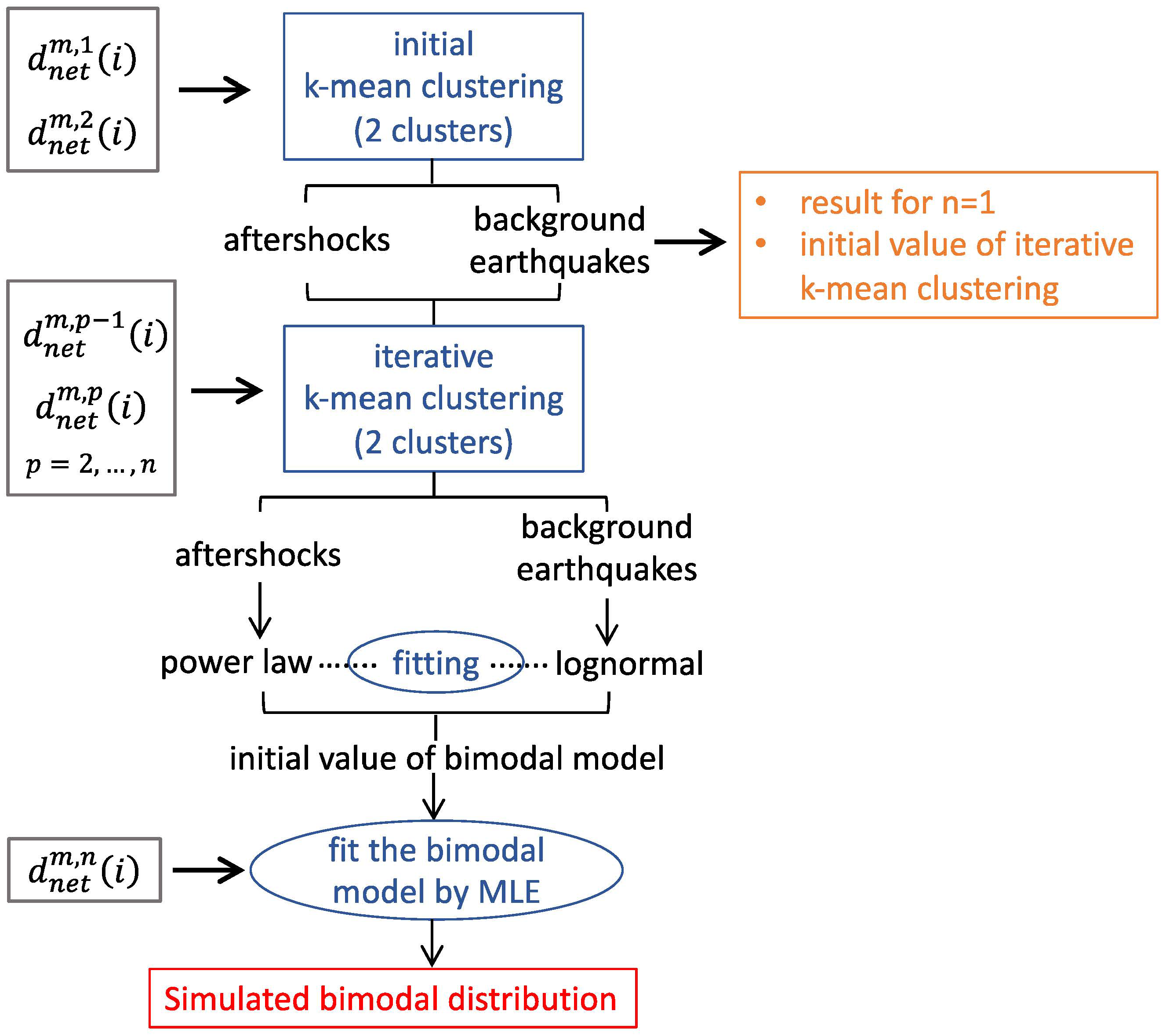
Specifically speaking, each earthquake is linked to its subsequent equal-magnitude events within a flexible time window in the definition of network distance; in this manner, the earthquakes are not presumed to be background earthquakes or aftershocks at the first stage, but their linkages are discussed. Next, the k-means clustering is introduced to categorize the network distance into two groups: the group with shorter network distances may be mostly contributed by aftershocks and the other with longer network distances is likely associated with the background earthquakes. Considering a bimodal distribution composed by the power law at shorter network distances and lognormal distribution at longer network distances can be observed in the frequency distribution of network distances. The network distances in the aftershock and background earthquake groups are respectively fitted by power law and lognormal distribution to obtain the initial guess of the bimodal model. By this way, the parameters controlling the model would be determined by the data.

2. Network Distance and Interevent Distance

To identify the universality of the spatiotemporal relationship, we selected earthquake catalogs from the following well-operated seismic networks: the California Integrated Seismic Network: Northern California Seismic System and Southern California Seismic Network in California and the Central Weather Bureau Seismic Network (CWBSN) in Taiwan. We chose the time span of 1 January 2001 to 31 August 2021 and targeted earthquakes within a magnitude interval 2.0 to 5.0; earlier time periods were associated with issues of incomplete data. 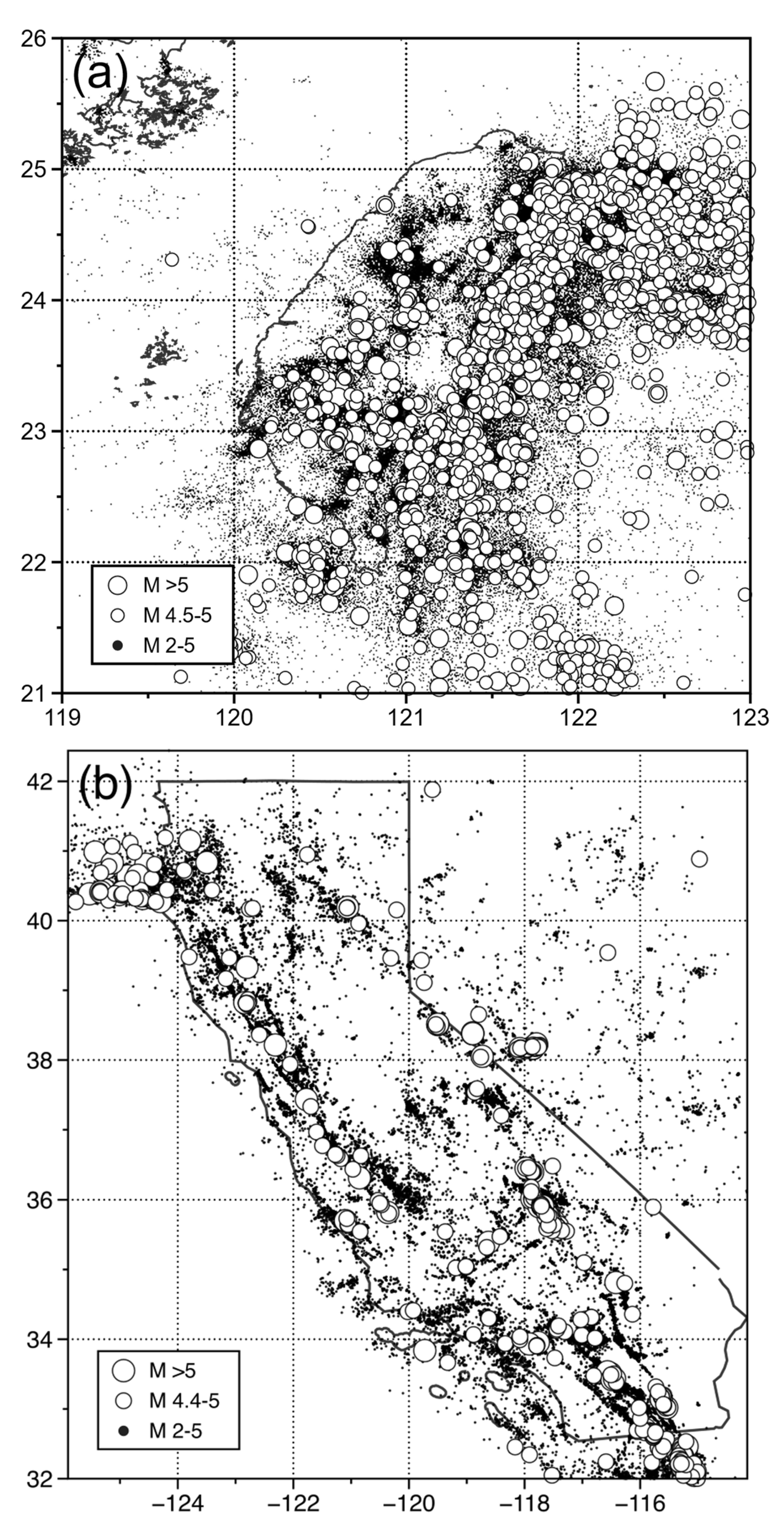Figure 1 shows the seismicity included in the calculation in each region. A higher seismicity rate contributed by 591,097 events over the area of 36,197 km² can be observed in Taiwan (Figure 1a), compared with that that consists of 84,384 events over the area of 423,970 km² in California (Figure 1b).

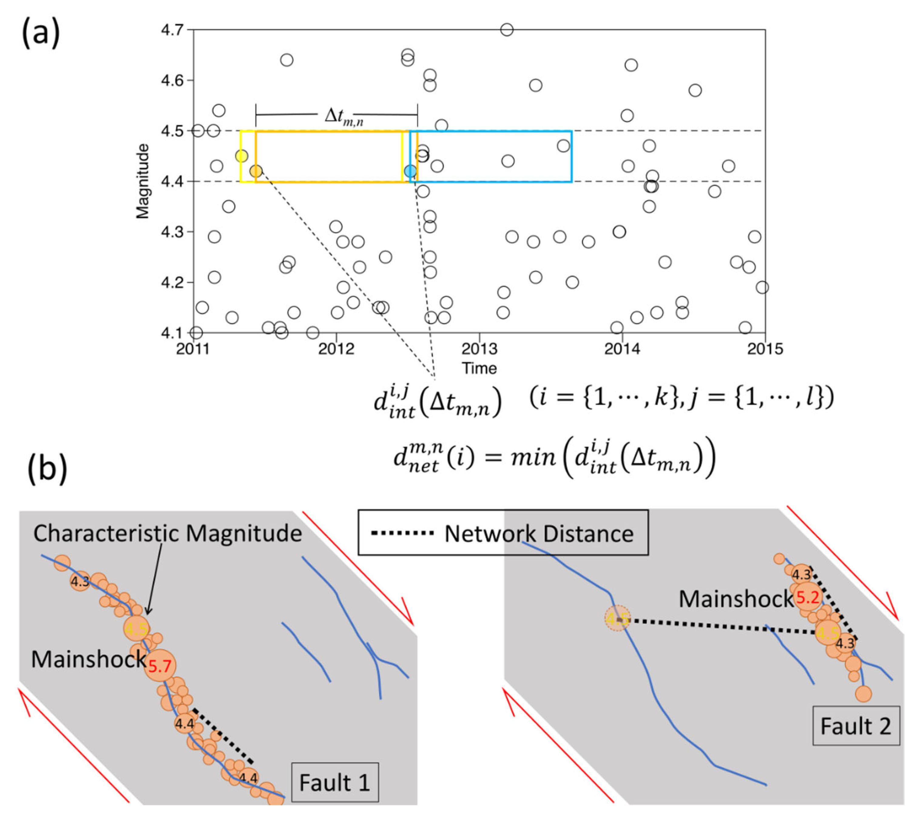
With the targeted earthquakes classified at magnitude intervals of 0.1, we calculated the distances between each event and their subsequent events of “equal” magnitude occurring within a given time window. This time window was defined as $\Delta t_{m, n}={10}^n\Delta t_m$, where $\Delta t_{m,0}=\Delta t_m$ is the average interevent time for specific magnitude m and n lying between −2.0 and 1.0 at intervals of 0.1. The different values of n correspond to the scales to zoom in or zoom out of the average interevent time. Assuming the number of events of magnitude m is k and the number of those in a time window $\Delta t_{m,n}$ is l, the interevent distance for the ith event in this time window would be defined as $d_{int}^{i,j}\left(\Delta t_{m,n}\right)=\left|\left(x_{j+1,}{y}_{j+1},z_{j+1}\right)-\left(x_{j,}{y}_j,z_j\right)\right|$, where $i=\left\{1,\cdots ,k\right\}$ and $j=\left\{1,\cdots ,l\right\}$ and the difference of the event time would follow $t_{j+1}-t_j\le \Delta t_{m,n}$, as illustrated in Figure 2a. The shortest interevent distance for ith event was set as network distance $d_{net}^{m,n}\left(i\right)$, some possible cases of which are given in Figure 2b.

As illustrated in Figure 2b, the interevent or network distance may represent the distance between aftershocks, mainshocks and aftershocks, triggered earthquake and its aftershocks, and background earthquakes. For aftershocks, the network distance mostly takes events with magnitude smaller than characteristic magnitude occurring on one single fault into account and is therefore confined by the rupture length. For background earthquakes, the network distance can be the distance between earthquakes that occur either on the same fault or on two adjacent faults in a local fault network; in most cases, the former should be considerably less than the latter, since energy is released when an earthquake occurs and the fault will not proceed through the next rupture until sufficient stress is accumulated over the interevent time. As such, the longer network distances may be more associated with the distance between faults, that is, the dimension of the local fault network. Generally, the number of network distances between aftershocks overwhelms the other network distances, and thus, the distribution of the shorter network distance majorly shows the properties of aftershocks.

3. Frequency Distribution of Network Distance

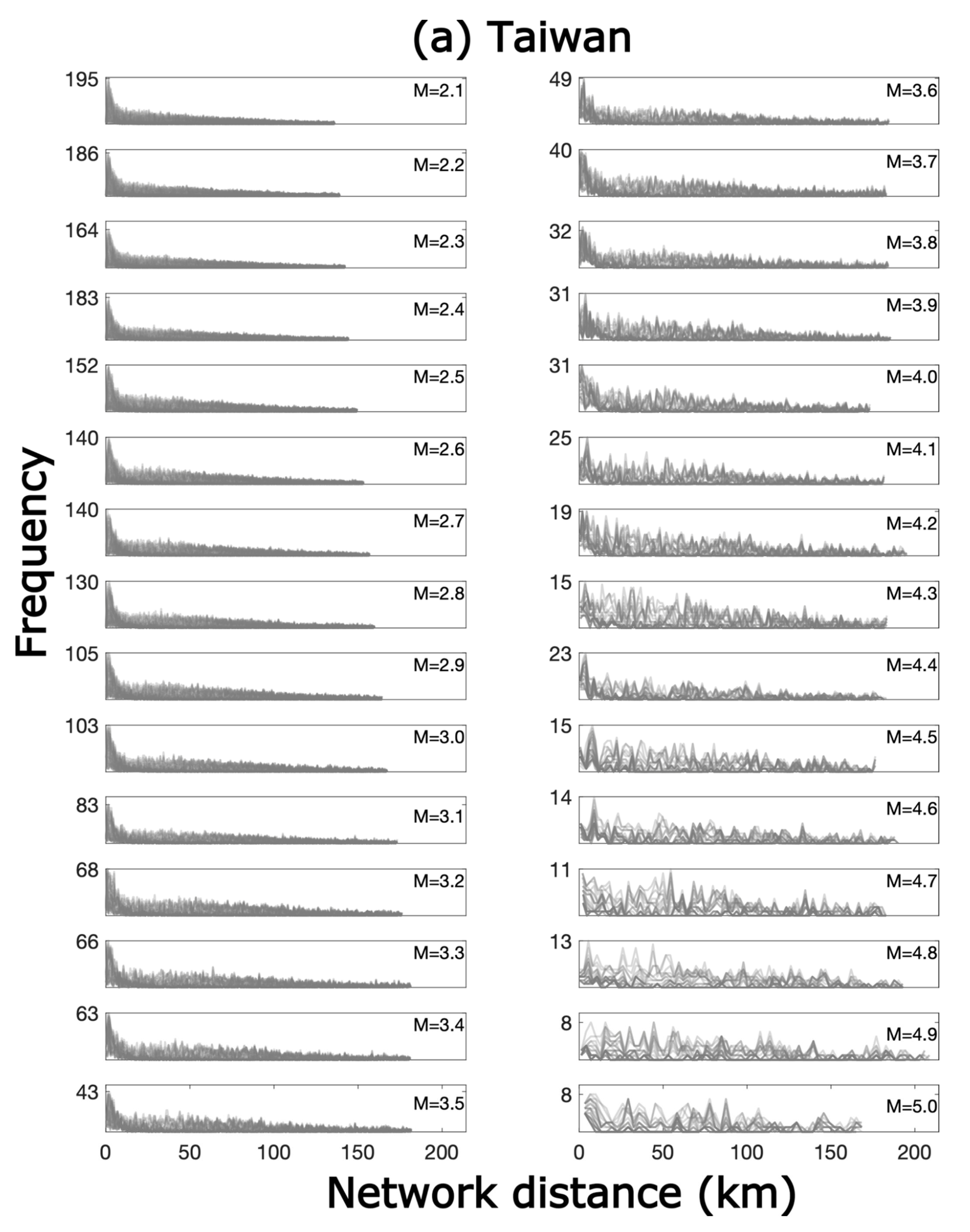
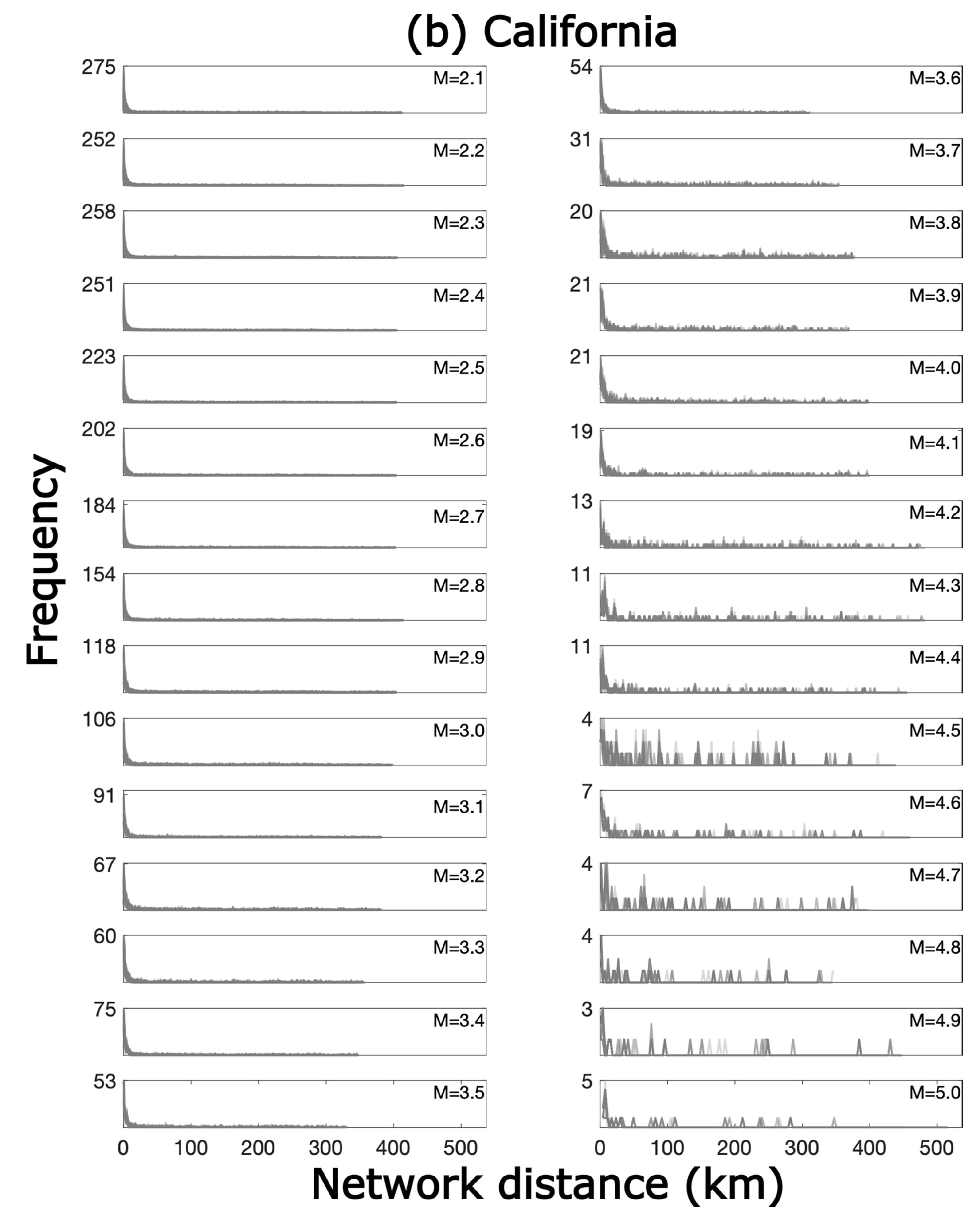
We studied the frequency distribution of network distance with different time window $\Delta t_{m,n}$ at different magnitudes (Figure 3). The distances between large earthquakes are inherently longer than those between small earthquakes, and the frequency of large events is much lower than that of small earthquakes. To more effectively describe the frequency distribution of the network distance, it requires a variable bin length that depends on the magnitude.

The rupture length scaled with magnitude was adopted to determine the appropriate bin length for the frequency distribution, as most network distances are those between aftershocks, and thus, the rupture length is somewhat correlated with the network distances. Following the relation of subsurface rupture length and magnitude for all slip types reported by Wells and Coppersmith (1994) [30] and Leonard (2010) [31], $\log \left(\mathrm{RLD}\right)=-2.44+0.59M$, the subsurface rupture length (RLD) in units of km was taken as the bin length for M = 5.0. However, the rupture lengths of smaller magnitudes of 2 to 3 are not clearly documented. To obtain a reasonable bin length for M = 2.1, we tried different bin lengths in the frequency distribution of network distance, ranging from 0.05 to 1.2 km resulting from empirical relationship of Well and Coppersmith (1994) [30] and Leonard (2010) [31], and obtained an appropriate bin length of 0.1 for M = 2.1. Taking the bin lengths for M = 2.1 and M = 5, the bin length d for the other magnitude bin was obtained using the scaling relation $\log \left(d\right)=a+bm$, where a and b are constants.

To avoid the estimation being biased by the long flat tail caused by extreme events, the frequency distribution was truncated at the network distance one standard deviation above the mean. The frequency distributions of network distance with different $\Delta t_{m,n}$ values for each magnitude are shown in each panel in Figure 3. Two distributions can be observed in the frequency distribution; one is the power law and the other is plausibly the lognormal distribution.

4. Power Law and Lognormal Distribution of Network Distances

The frequency distribution of network distance in Taiwan (Figure 3a) shows the characteristics of a power law distribution with a high peak in the short network distance (<10 km) region and a long tail, similarly to the Gutenberg–Richter law or the modified Omori law. Meanwhile, the increased frequency at the median network distance (<150 km) may suggest a distribution that is controlled by the physics of background earthquakes. A natural system such as a fault system is always proceeding toward maximum entropy under the condition of least-informative default. From this point of view and the distribution shape, we presumed that a lognormal distribution presenting the multiplicative product of many independent random variables may be able to describe the development process of the background earthquakes.

To distinguish the data from different distributions, we subjected the network distance series into k-means clustering [32] to group them into aftershock and background earthquake clusters. We then fit the data in the aftershock cluster using the power law distribution and those in the background earthquake cluster using lognormal distribution. In the end, these two distributions constructed a bimodal distribution as follow:

$$y\left(x\right)=p\times a{x}^b+\left(1-p\right)\times \frac{1}{x\sigma \sqrt{2\pi }}exp\left(-\frac{{\left(\log x-\mu \right)}^2}{2{\sigma }^2}\right)$$

(1)

where p is the probability of success in explaining the data using the power law, a and b are constants in the power law distribution, and $\mu$ and $\sigma$ are the mean of logarithmic variable values and standard deviation in the lognormal distribution. Since aftershocks and background events are exhaustive and mutually exclusive possibilities, the probability of failing to predict using the power law inherently translates to the probability of successful prediction using the lognormal distribution. A flowchart and detailed description of the above steps is shown in Figure 4.

Note that the events with different magnitude consist of both aftershock and background earthquakes and would contribute a large range of network distances and therefore lead failure of k-mean clustering. Furthermore, another purpose of this study is to search for the characteristic magnitude. As hierarchical analysis reduces the complexity of analysis, therefore, the network distances are grouped according to different magnitudes and are then analyzed. The whole process results in the simulated bimodal distribution as the above equation. 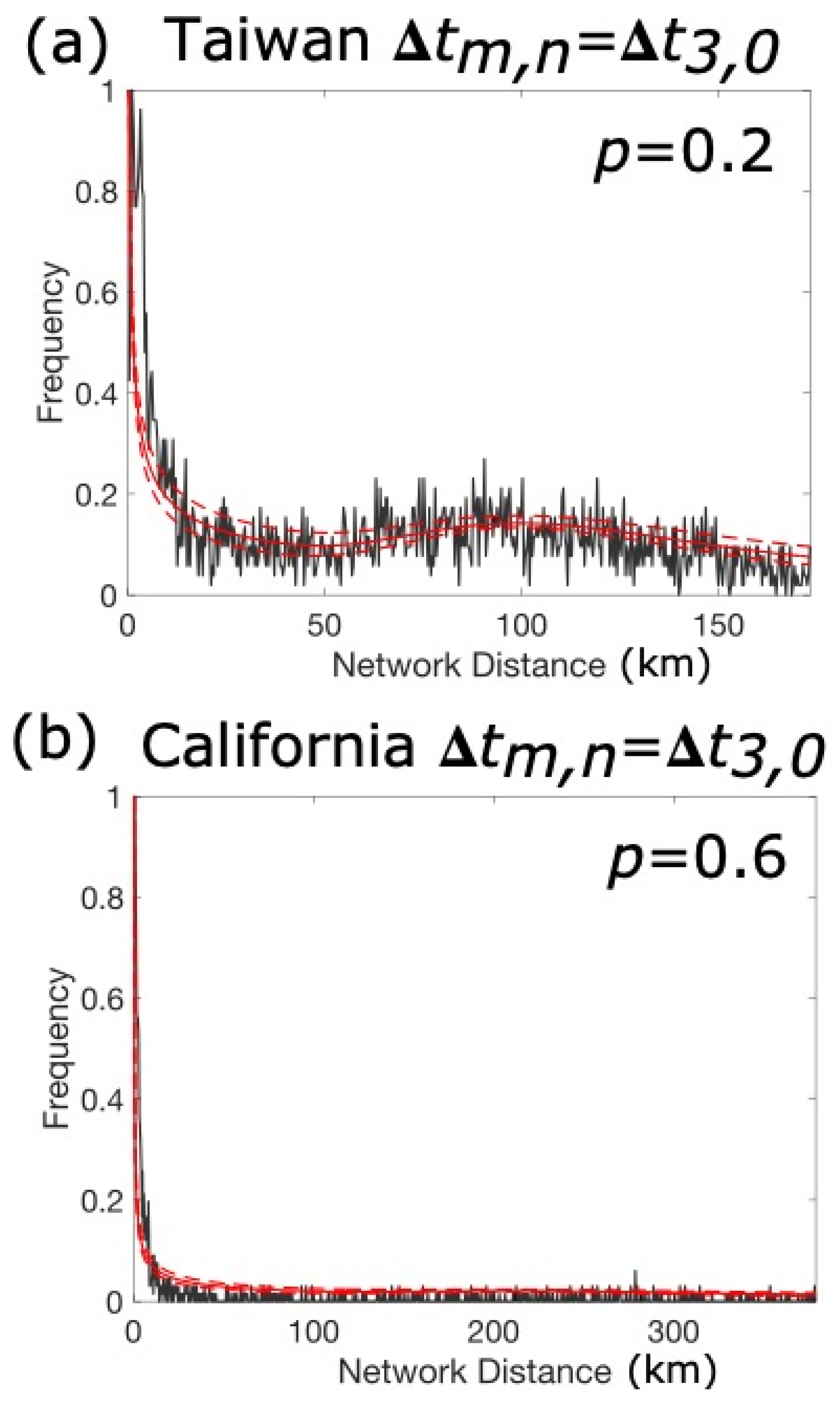Figure 5 shows one of the fitting results for Taiwan and California using the events with magnitudes in between 3.0 and 3.1 occurring within the average interevent time of this magnitude. The bimodal distribution starts from the lower limit of the power law and then shows another peak around the mode of the lognormal distribution.

5. Spatiotemporal Relationships of Aftershocks and Background Earthquakes

The relationships of the network distance with magnitudes were obtained for the aftershocks and background earthquakes by calculating their mode of the network distances, giving specified magnitude m and time window n, as shown in the top panels of Figure 6. The curves in the top panels of Figure 6 show the comparison of the relationship with and without presuming an interevent time (red curves and black curves), as well as the comparison of the outcome from true events (red and black curves) and from the fitting result (blue curves). We picked the maximum network distance (black curves in top panels and circles in bottom panels of Figure 6) among those of 31 different time windows for the purpose of investigating the longest distance in the fault network at which one event is linked to another one of equal magnitude. The network distances of aftershocks and background earthquakes discriminated from k-means share similar trends in the Taiwan and California regions. For aftershocks, the network distances obtained in different means gradually converged to the same value until the magnitude increased to a characteristic magnitude (magnitude group I to III of top-left panel of Figure 6 in each region); for background earthquakes (top-right panel of Figure 6), the curves show similar increases or even trend in magnitude group I, but the fitting results start to present a reverse trend with the real data for magnitude group II.

With the goal of studying the relationship between the time and the network distance for aftershocks and background earthquakes, we fit them using a power law (Figure 6, bottom panels). The times presented here result from the interevent times of events with a particular time window and magnitude $\Delta t_{m,n}^{af/bg}\left(j\right)$; the interevent times smaller than the median were collected ($\Delta {\tilde{t}}_{m,n}^{af/bg}=\Delta t_{m,n}^{af/bg}\left(j\right)\le median\left(\Delta t_{m,n}^{af/bg}\left(j\right)\right)$), and the mean of these interevent times $mean\left(\Delta {\tilde{t}}_{m,n}^{af/bg}\right)$ present the average interevent time for the specific time window and magnitude. Finally, the mode of the average interevent times for each magnitude was calculated and presented as the time in the bottom panels of Figure 6. The results showed a better fit with a higher coefficient of determination R² for Taiwan than for California, and a better fit for background earthquakes than aftershocks. In addition to that, the fitting produced the best R² value when considering all the magnitudes of aftershocks, but this was not the case for background earthquakes. The regression showed better fittings for background earthquakes only when considering the magnitudes smaller than a characteristic magnitude of 4.5 for Taiwan and 4.3 for California.

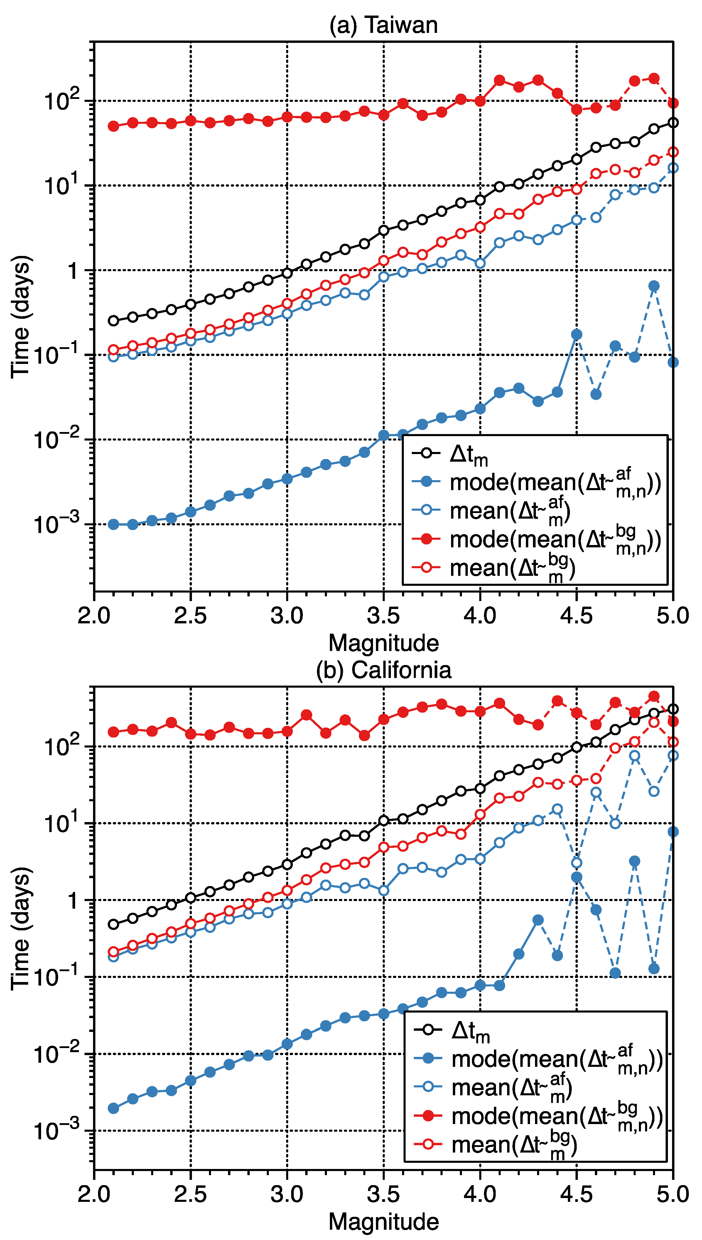
In addition to the relationships of the network distance, we examined the average interevent time of all events $\Delta t_m$ and its relationship with the interevent time of aftershocks and background earthquakes (Figure 7). One of the interevent time of aftershocks and background earthquakes was calculated following a previously mentioned method; furthermore, we also calculate the average interevent time of aftershocks and background earthquakes. As shown in Figure 7, the average interevent times of all events, aftershocks, and background earthquakes have similar results in both Taiwan and California; however, the average interevent time usually considered in most forecasting or statistical models is overall larger than the average interevent time of aftershocks and background earthquakes. Moreover, this is merely the situation for presuming the average interevent time as time window in the network distance calculation; the actual interevent time of aftershocks and background earthquakes shown as the solid circles in Figure 7 can be biased from the average interevent time of all events more when without presuming a time window of average interevent time. Their relation implies that the interevent time may have been overestimated in some empirical studies, especially when talking about aftershocks. However, the interevent time of background earthquakes may have been underestimated.

6. Discussion and Conclusions

We essentially divided the seismicity into two categories: aftershocks and background earthquakes. However, in our method used for network distance calculation, aftershocks may actually include any triggered seismicity such as foreshocks or swarms and even background earthquakes. These seismic activities may differ in their triggering mechanism, but they share one common point of being strongly coupled or linked. The linkage may be in time or in space. Therefore, the k-means or other clustering methods may be applicable to aftershocks here to gain insight into different types of seismic activity. In this study, we primarily focused on an average and stationary effects of triggering and on isolated background earthquakes that are not triggered.

The network distances of aftershocks show significant differences from that of background earthquakes that specify the different linking relationship between the events (Figure 6). The network distances of aftershocks show a similar trend and small differences, whether presuming the average interevent time as time window or not and can be fit well by the power law distribution. By contrast, the network distances of background earthquakes show large differences in the calculations with different conditions, although they share a similar trend, and the lognormal distribution only shows a similar trend for small to moderate magnitudes. Note that the results of the fitting of aftershocks by the power law and fitting of background earthquakes by lognormal are initial guesses of the bimodal model and do not represent the fitting results of the bimodal distribution.

A bimodal distribution formed by different patterns associated with background earthquakes and triggered earthquakes has been observed in interevent time distributions, spatiotemporal evolution, and simulations [33,34,35,36,37,38,39]. However, the lack of a well-described distribution for triggered or background earthquakes still remains, and most studies consider the interevent time only. Comparing the results from Taiwan and California (Figure 5), we demonstrated here that the bimodal distribution holds for different regions and different tectonic backgrounds for earthquakes. The bimodal distribution we proposed constitutes an alternative for describing seismicity consistent with a power law distribution for shorter network distances and a lognormal distribution for longer network distances. The parameter p in the bimodal distribution not only plays a role of probability of successful prediction of the aftershock cluster but also the mixture coefficient that would be adjusted in the iterative fitting.

Another common phenomenon observed in the cases of Taiwan and California is the overestimation of the interevent time for aftershocks and underestimation of that for background earthquakes, which is shown in Figure 7. The scaling law between the interevent time and magnitude showed a significant difference for aftershocks and background earthquakes when the time window is not presumed to be the average interevent time. This actually corresponds to the bimodal distribution of interevent time that has been reported in many regions [34,35,40].

In the case of Taiwan, the network distances other than the ones obtained from lognormal distribution grew with magnitude until a characteristic magnitude of 4.5 was reached for both aftershocks and background earthquakes (top panels of Figure 6). By contrast, the network distances in the case of California first show a flat trend in magnitude group I of aftershock and background earthquakes and then a plausible growth in the magnitude group II until the characteristic magnitude of 4.3. The values of characteristic magnitude were determined not only depending on the fitting result of the network distance but also for the interevent time results. Although the distribution of network distance versus time (bottom panels of Figure 6) seems to have better relation before the magnitude 3.9 and 3.7 for Taiwan and California, the results of power fitting show the best R² values for aftershocks when using the full range of magnitude, and the fitting shows the best R² values for background earthquakes when using magnitudes smaller than characteristic magnitude. In addition, the R² being lower in California than in Taiwan may be due to different magnitudes used in the Northern California Seismic System and Southern California Seismic Network and relatively lower seismicity rates in California, and lower R² for lognormal distribution because the number of long network distances are much less than the short ones, especially when the magnitude grows larger.

Another difference between the two regions is the values of the interevent time and the network distance. Although the average interevent times over all the data of each region were close, the interevent times obtained for aftershocks and background earthquakes with or without presuming a time window were all shorter in Taiwan than in California, as were the network distances in Taiwan compared to those in California. These findings appropriately describe the higher seismic activity in Taiwan and align with the expectation associated with the shorter fault lengths in Taiwan.

In most earthquake forecasting or hazard assessment studies, the spatiotemporal parameters and mainshock–aftershock problems are primarily determined based on empirical experiments or average interevent times. Wu et al. (2015) [41] illustrated the roles played by these parameters in statistical models by revealing how different parameter values contribute to superior statistical models in different regions with the same target magnitude. Furthermore, statistical models generally take all earthquakes in a magnitude interval into account with fixed parameter values; smaller background earthquakes that belong to different earthquake systems may be included in these calculations. Our results suggest that all these parameters as input to statistical models, especially the interevent time, should be adjusted according to the event magnitude.