
Multi-Parameter Observations of Seismogenic Phenomena Related to the Tokyo Earthquake (M = 5.9) on 7 October 2021


 , , ,
, , ,
Abstract
1. Introduction
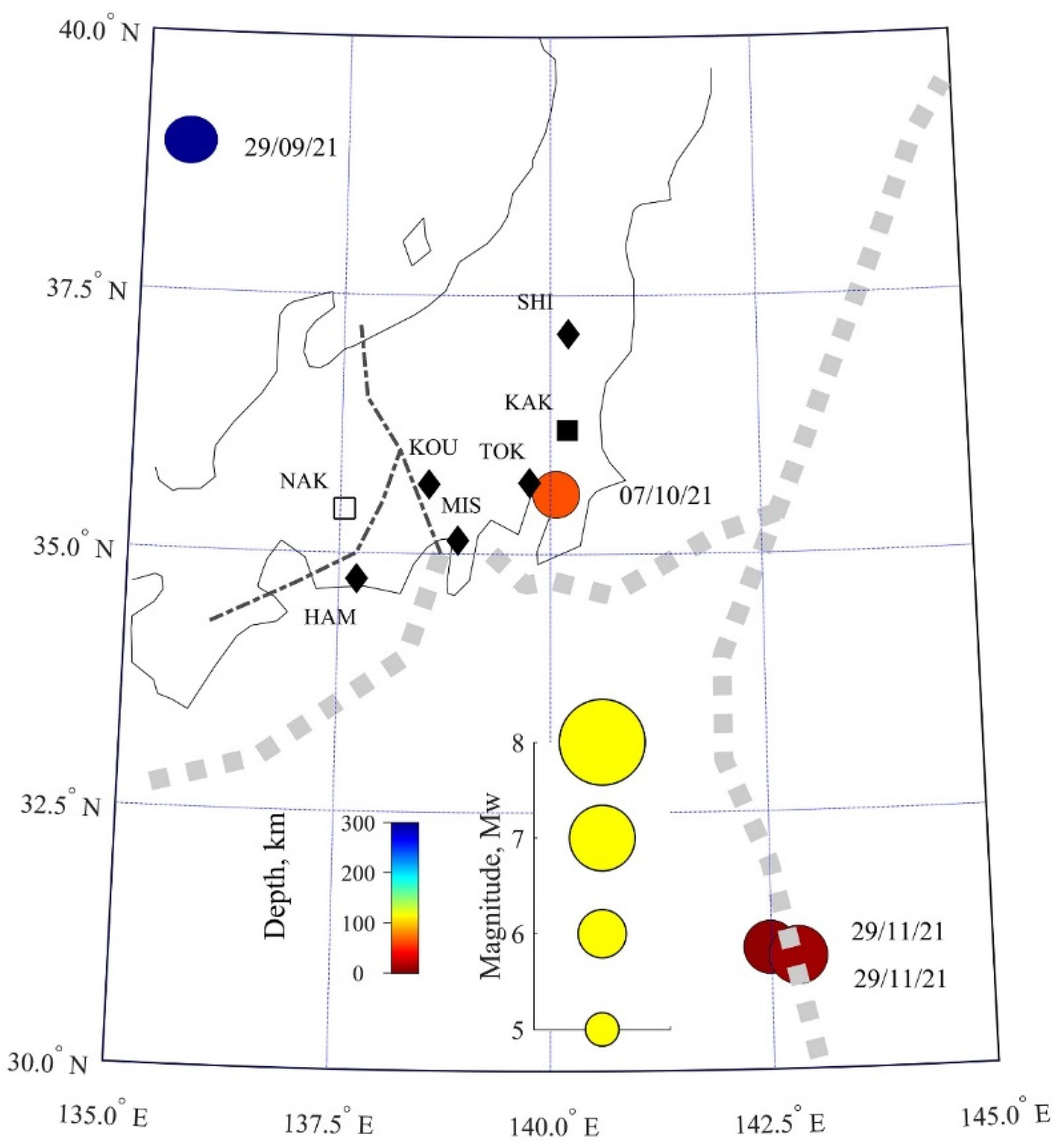
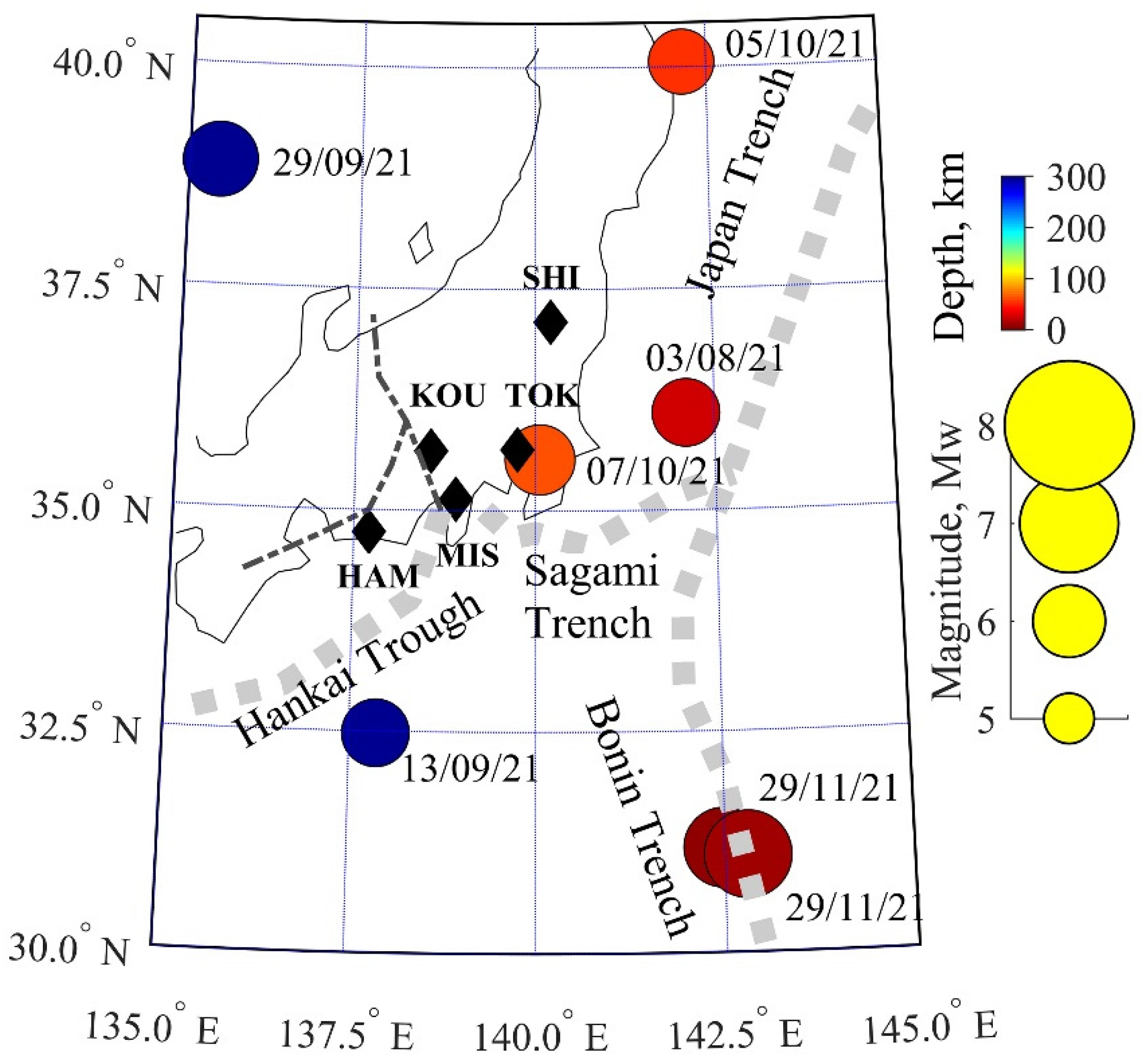
2. EQ Data
3. Observational Results
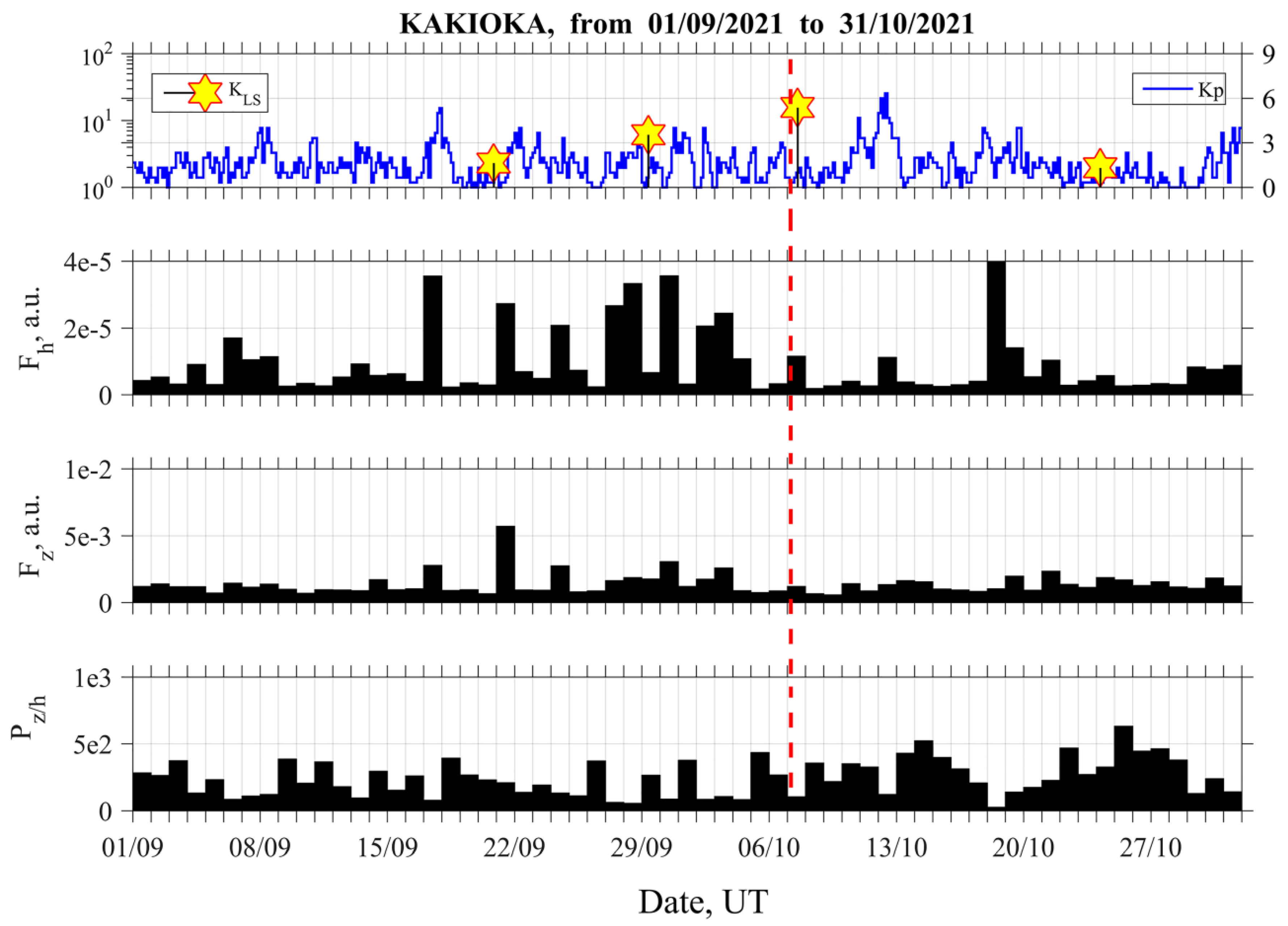
3.1. ULF Magnetic Field Observations
3.1.1. Data
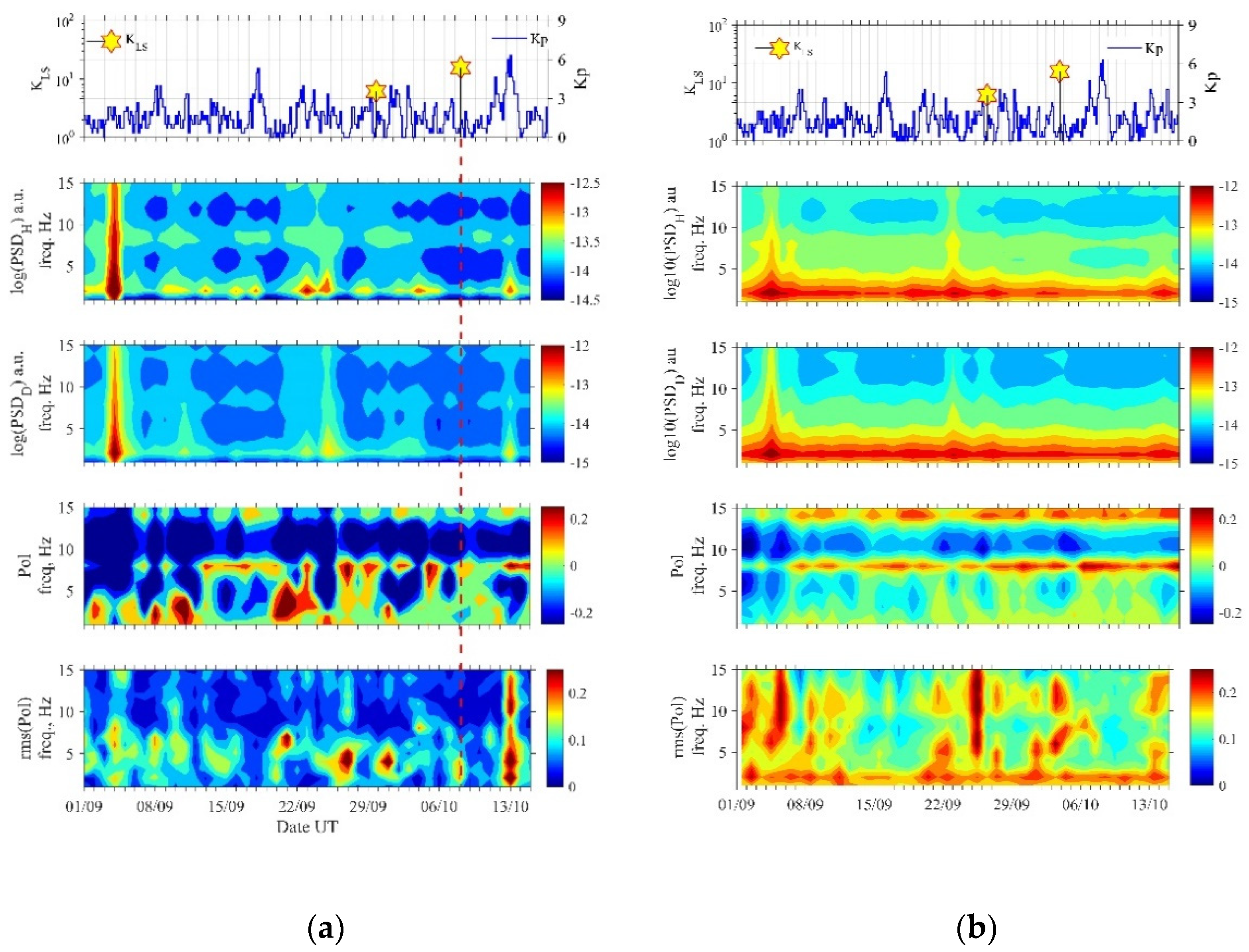
3.1.2. ULF Data Analysis and Results
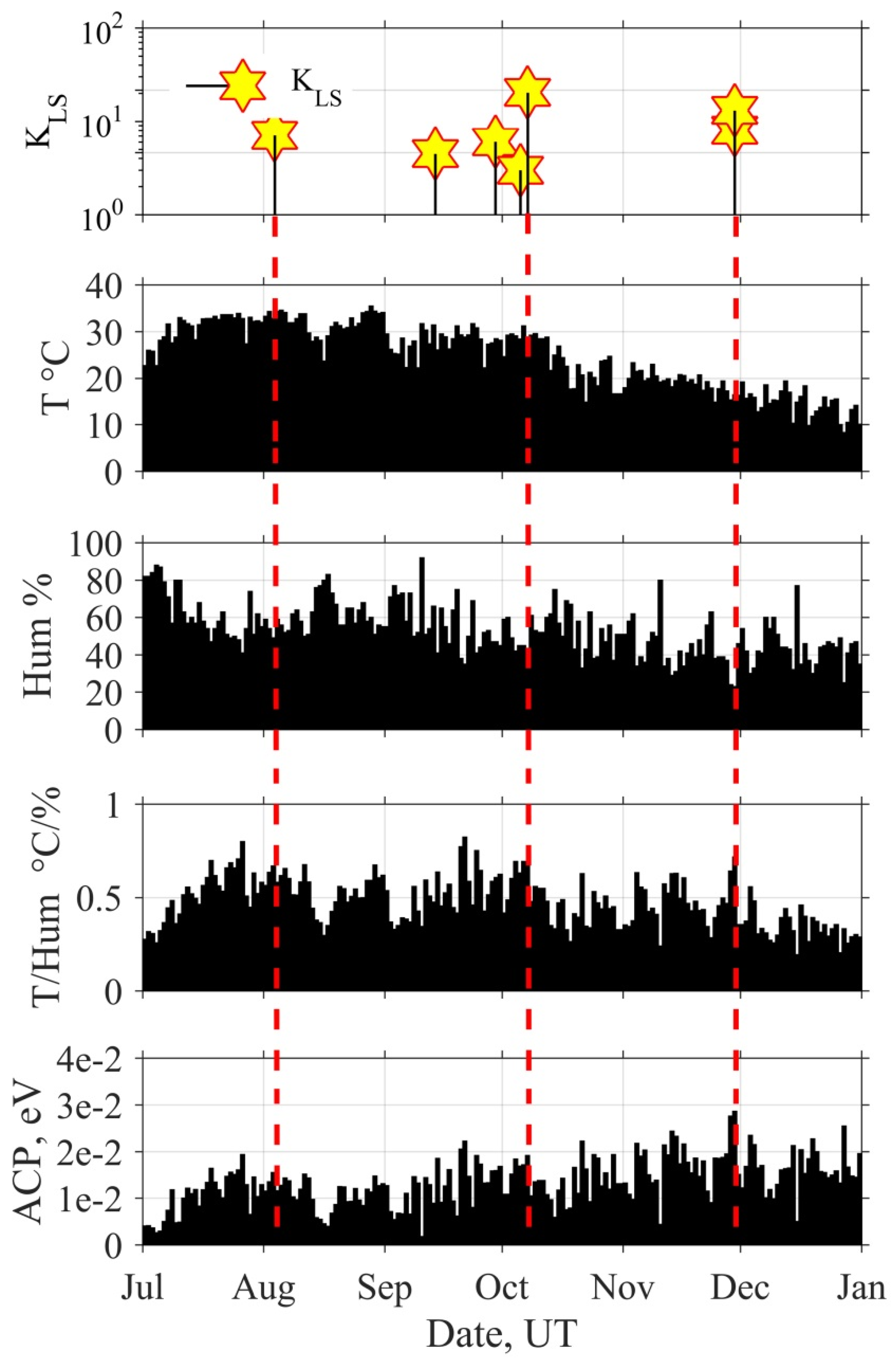
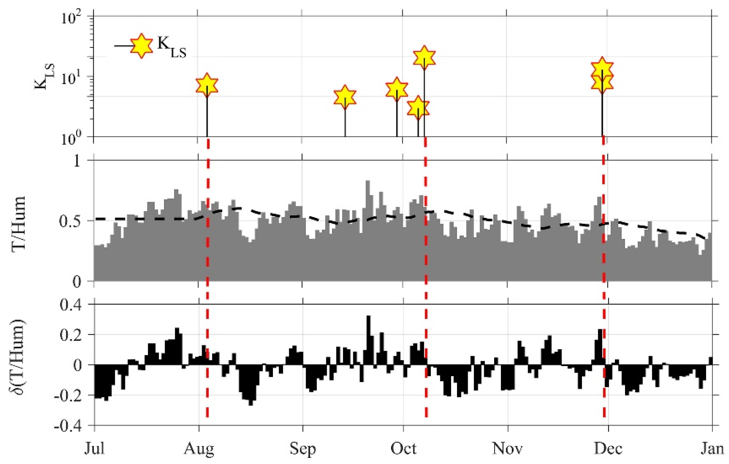
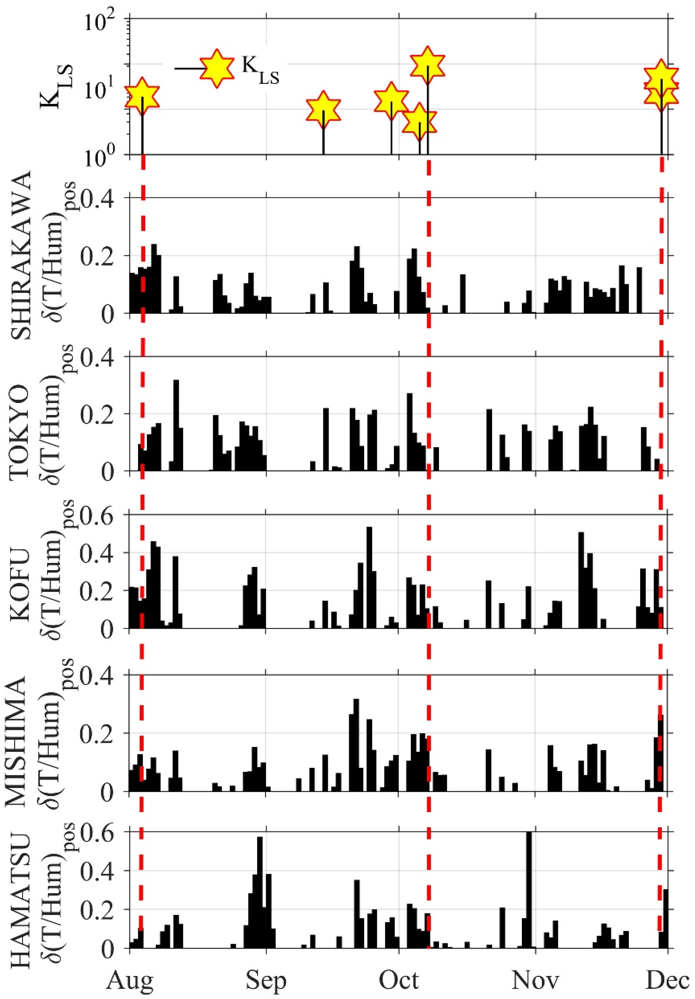
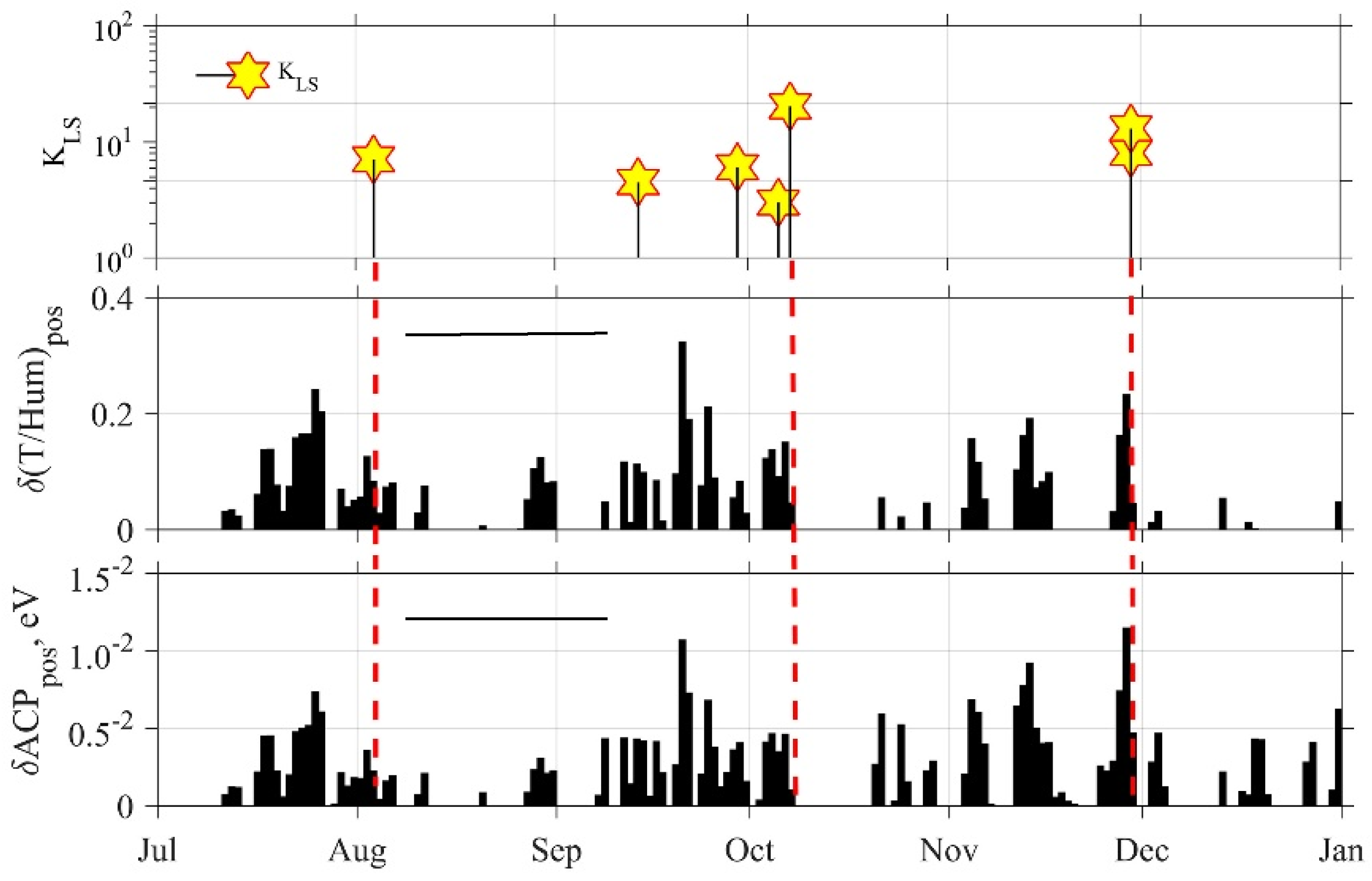
3.2. Meteorological Phenomena
3.2.1. Data and Processing
3.2.2. Analysis Results
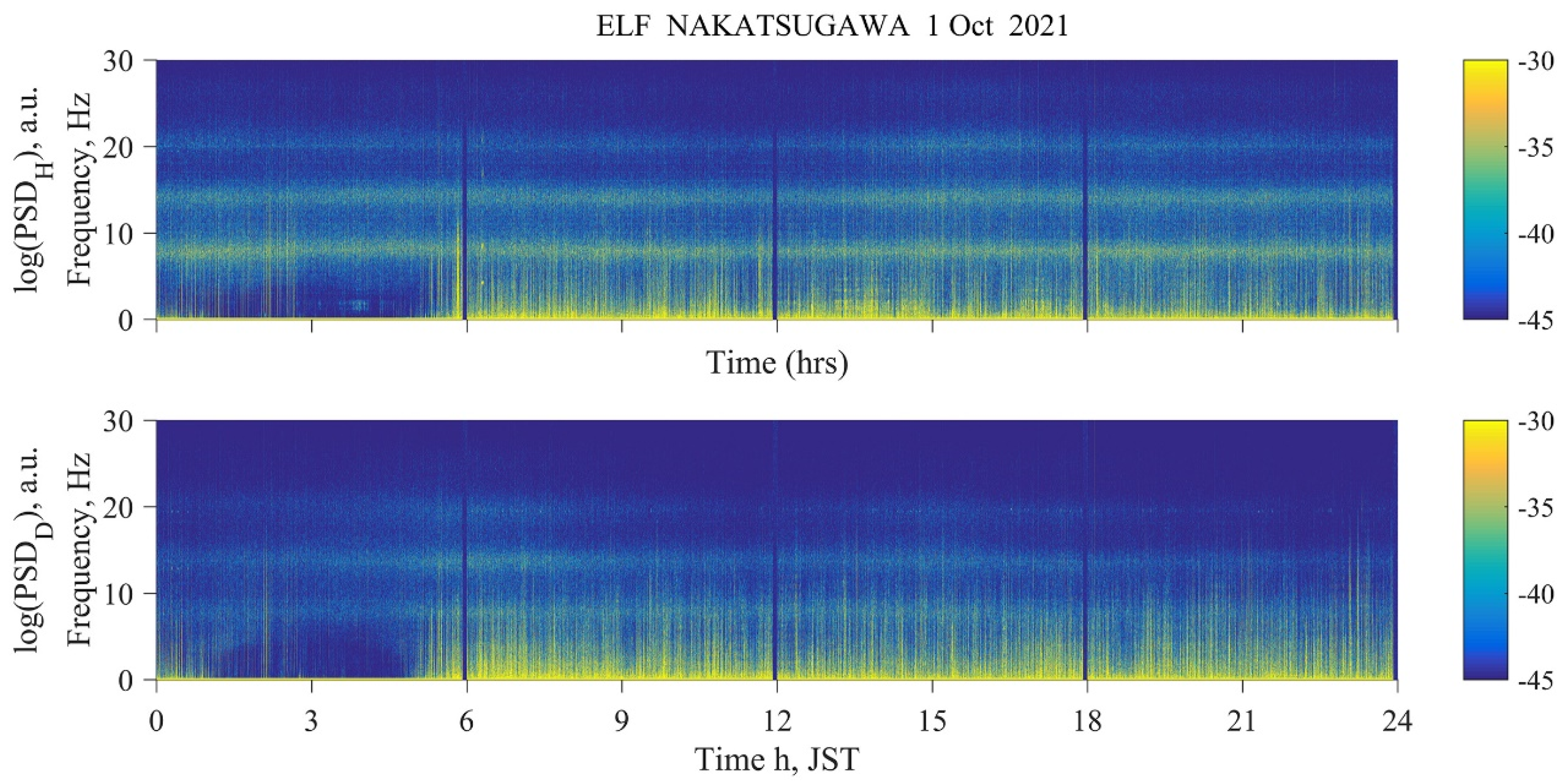
3.3. ULF/ELF Electromagnetic Radiation
3.3.1. Data
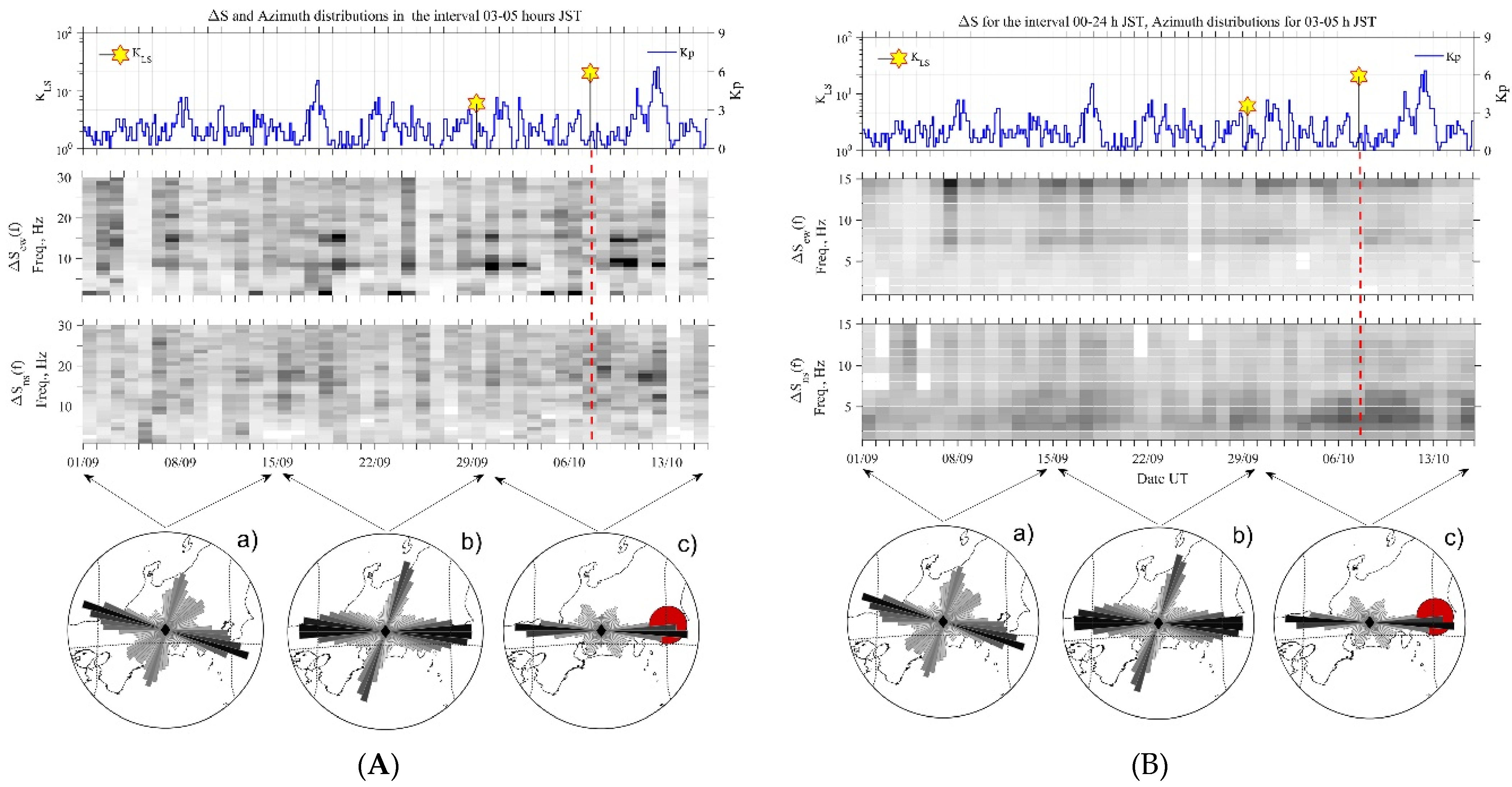
3.3.2. Analysis and Results
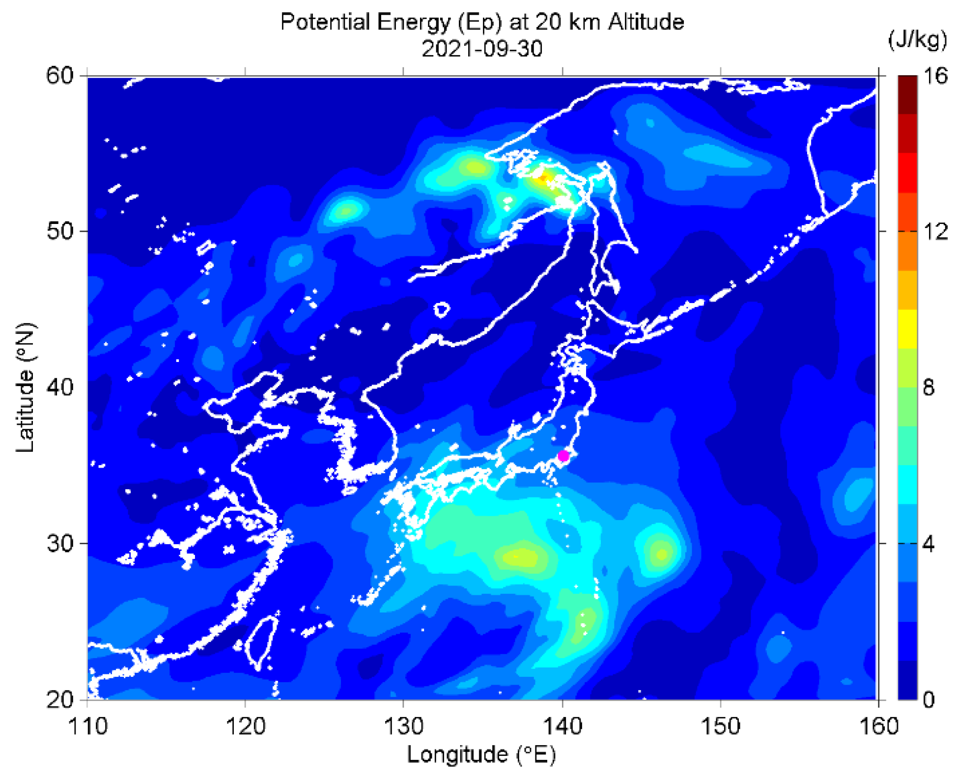
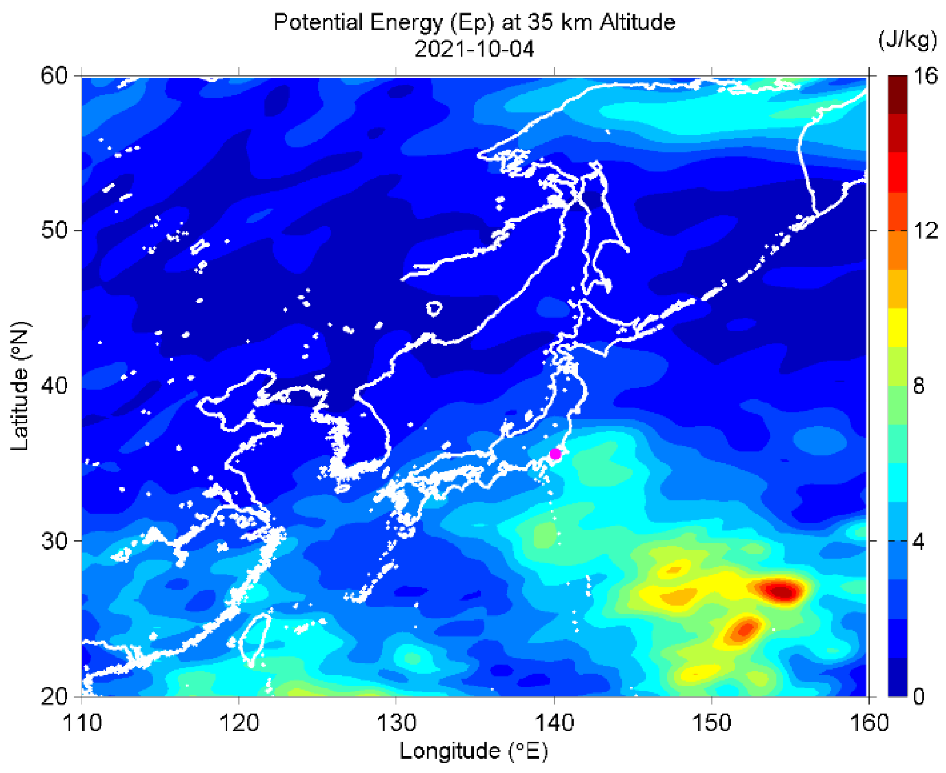
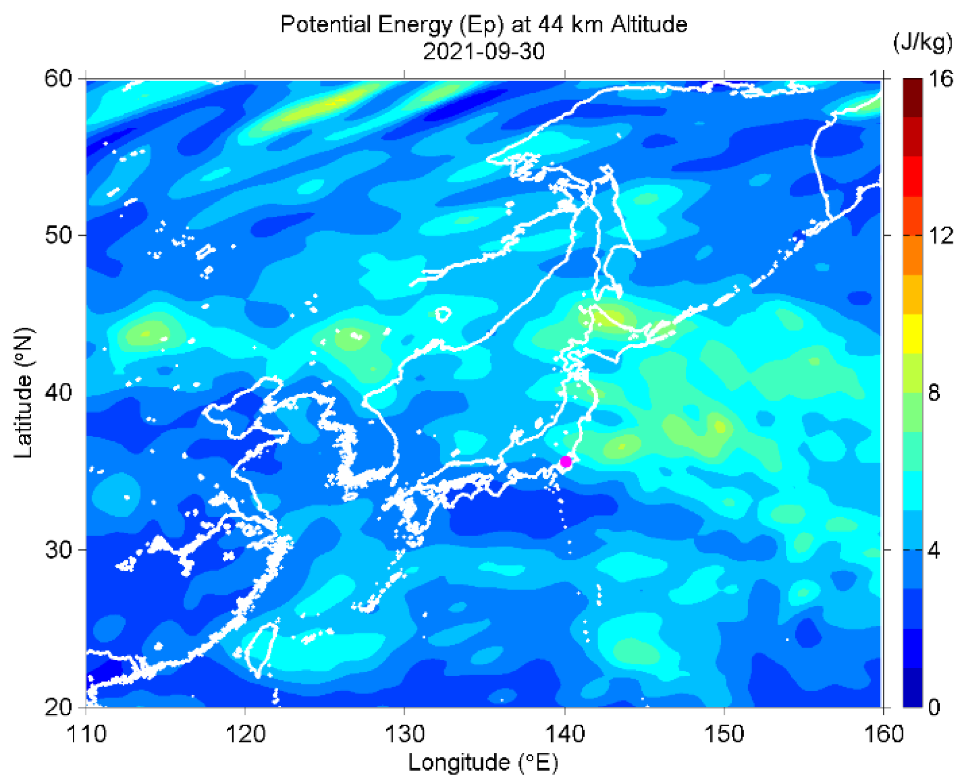
3.4. Stratospheric and Lower Mesospheric AGW Activity
3.4.1. Analysis Method
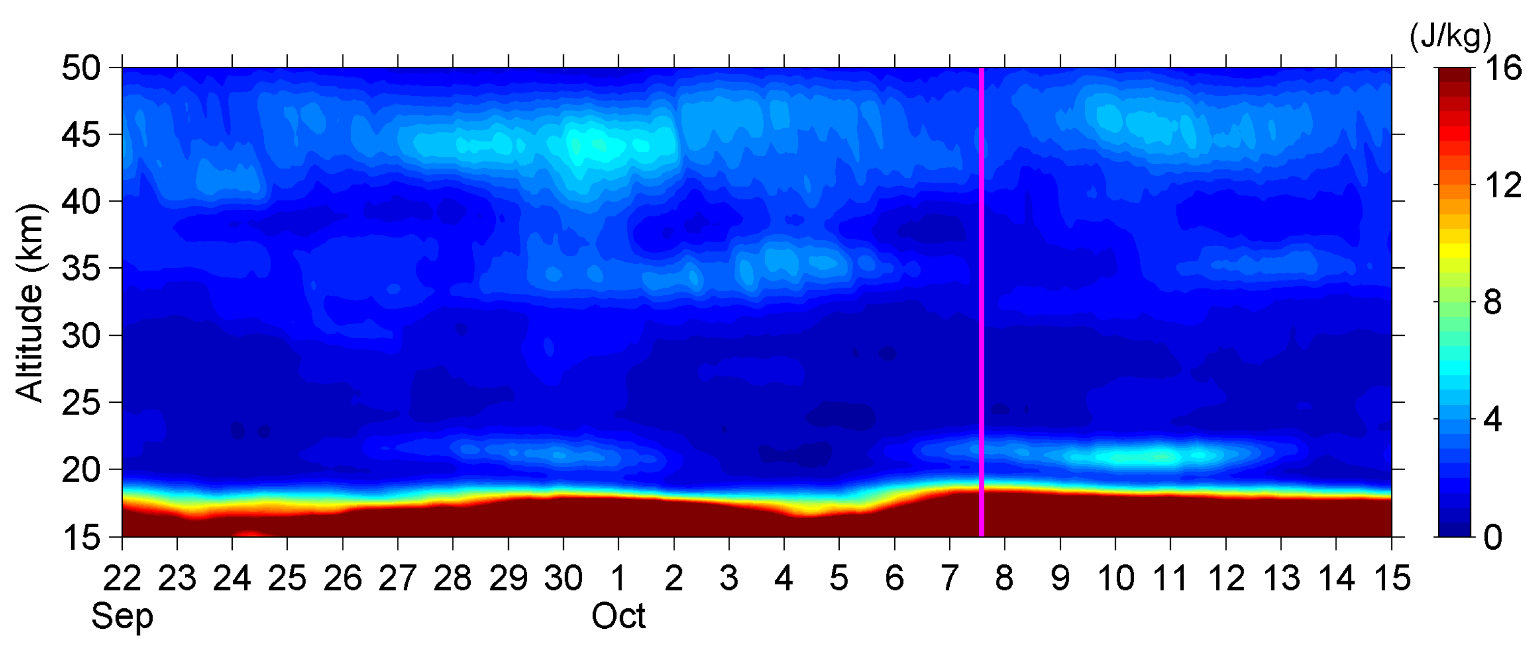
3.4.2. Observational Results
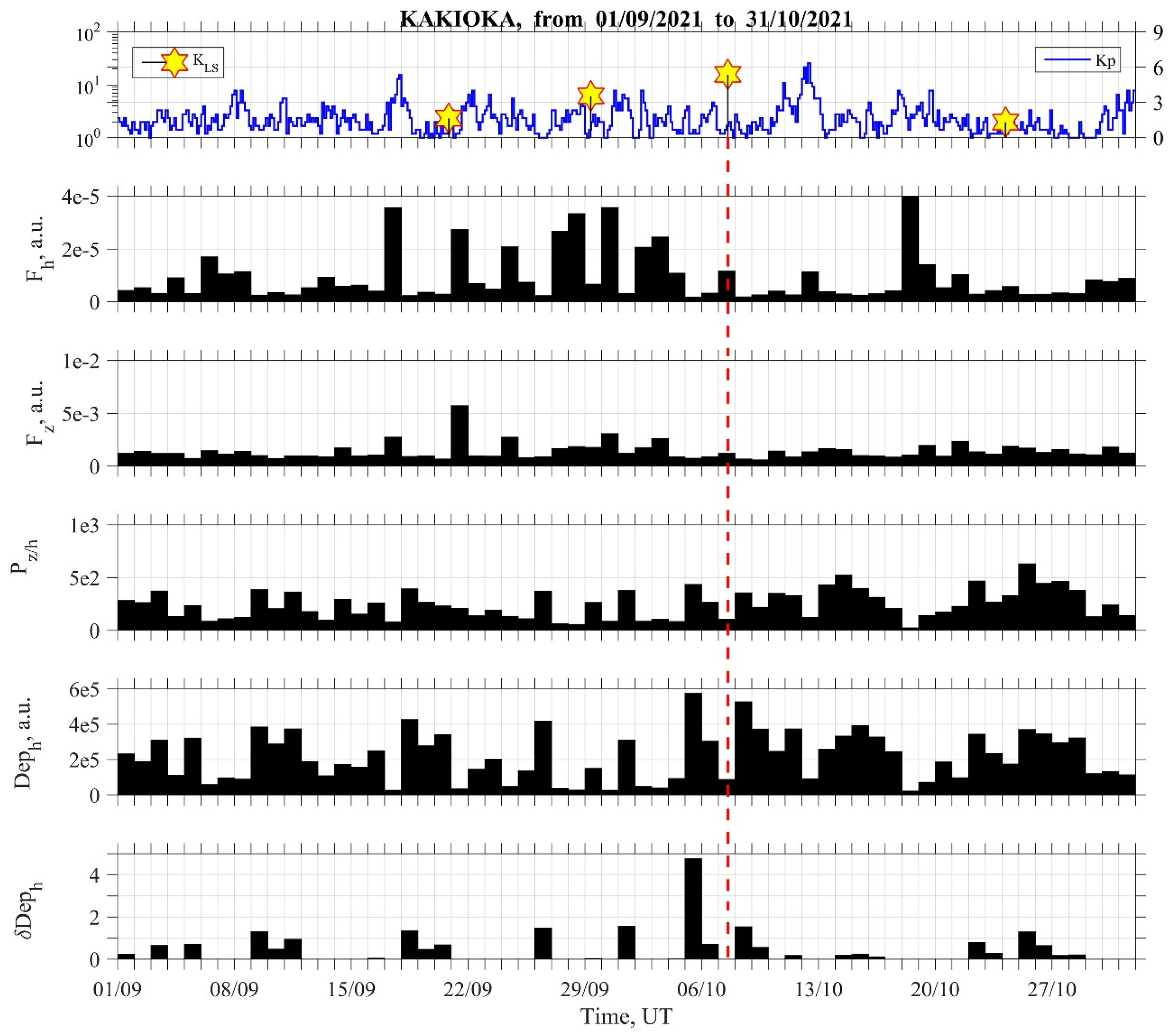
3.5. ULF Depression (Lower Ionospheric Perturbation)
3.5.1. Analysis Method
3.5.2. Analysis Results
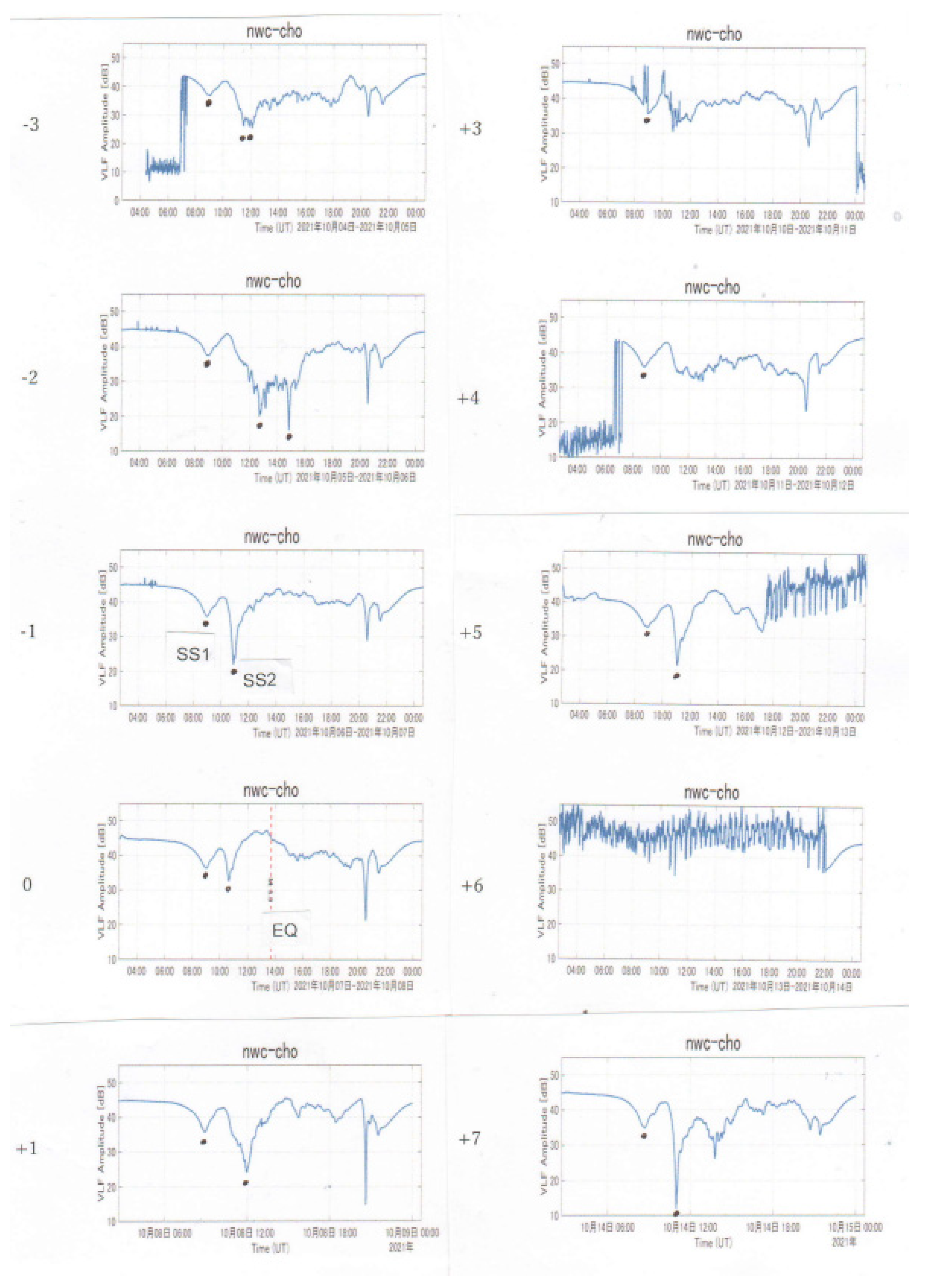
3.6. VLF/LF Subionospheric Propagation Measurements
3.6.1. Observational Results in Kamchatka
3.6.2. Observational Results in Japan
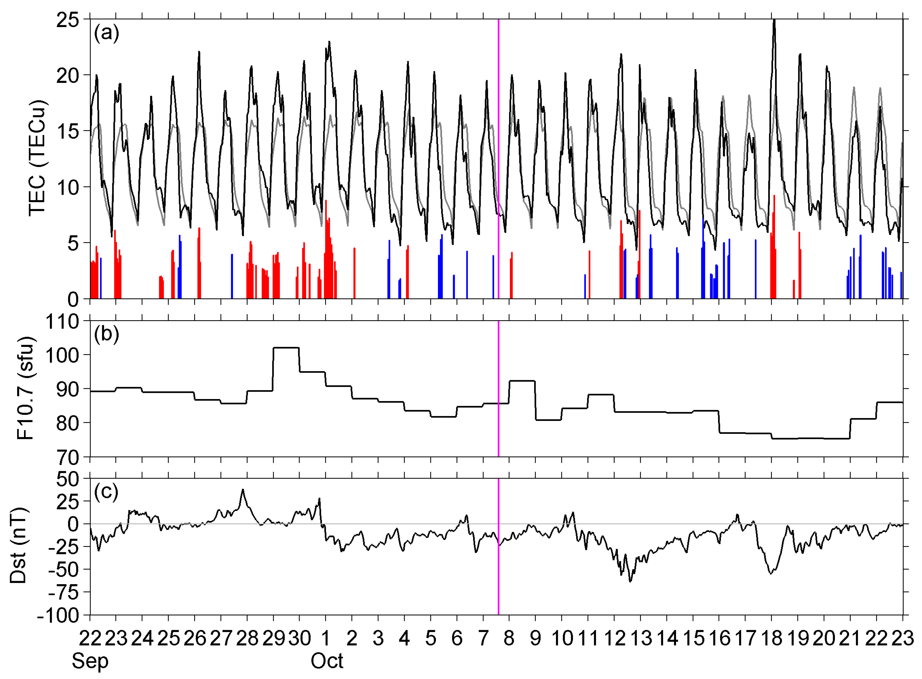
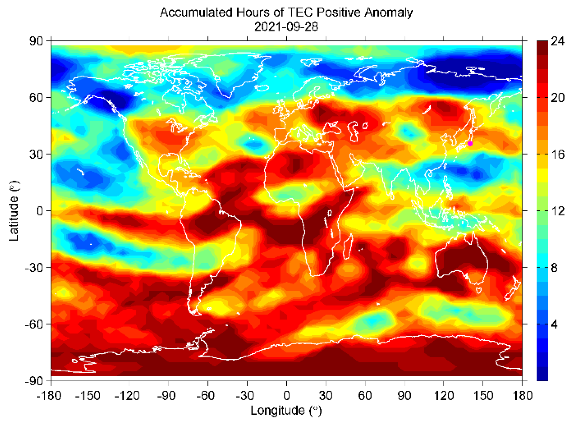
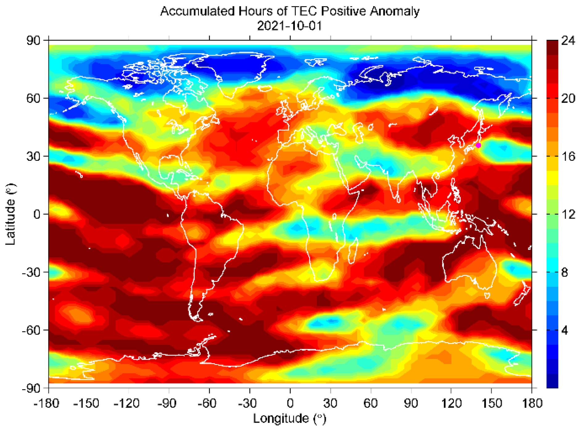
3.7. TEC (Total Electron Contents) Measurements
3.7.1. Analysis Method
3.7.2. Observational Results
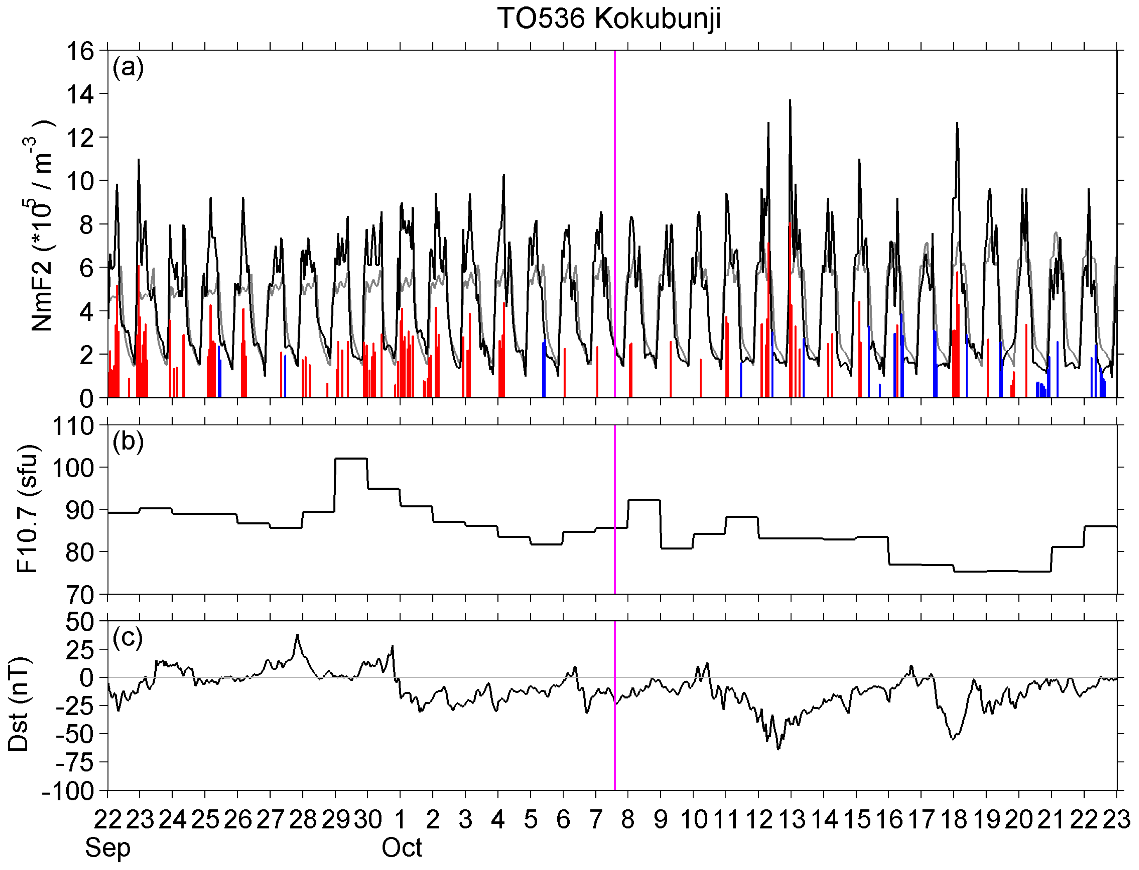
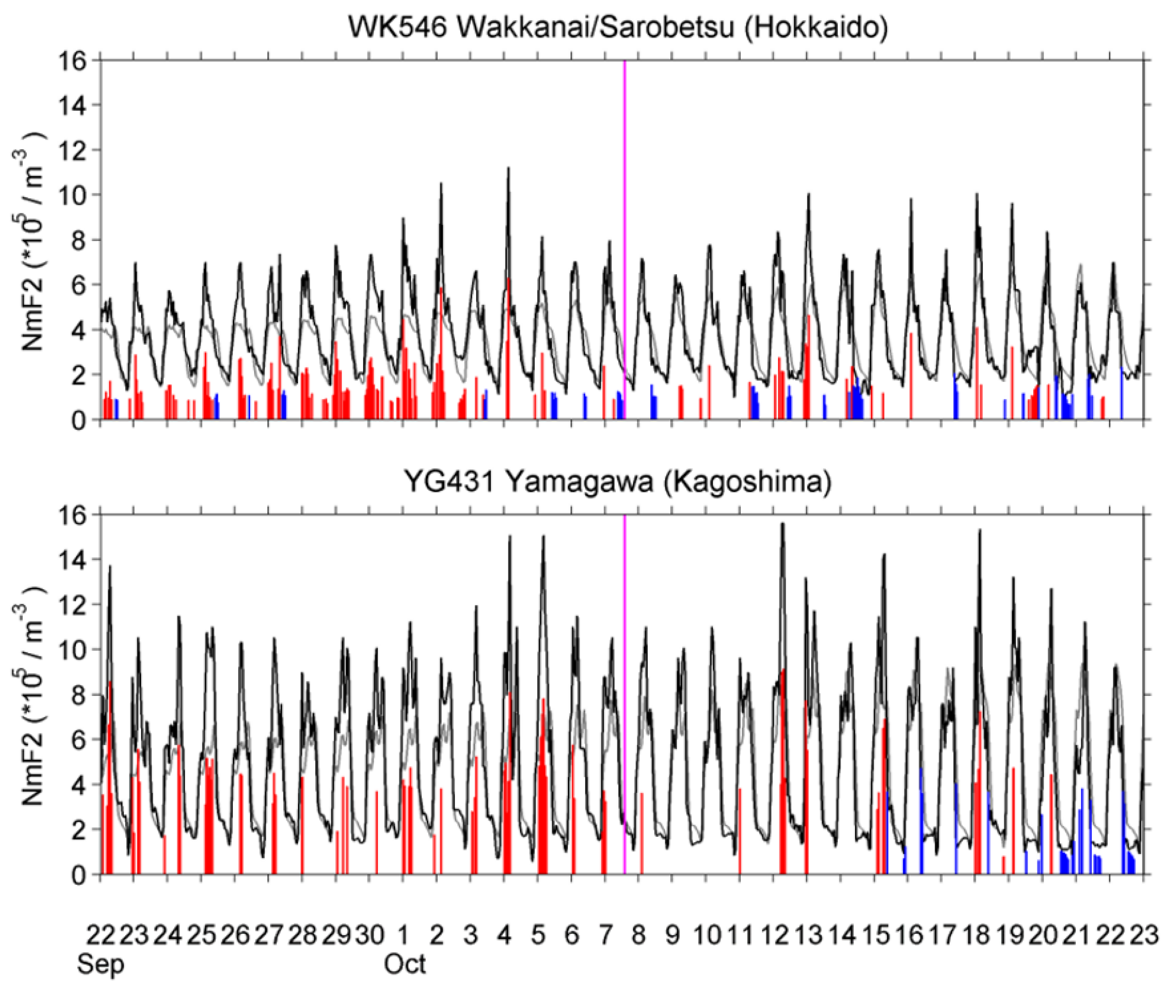
3.8. NmF2 Ionosonde Measurements
3.8.1. Data
3.8.2. Analysis Results
4. Summary and Discussion
- Lithospheric effects: Prior to large EQs, we understand that the electromagnetic radiation in the ULF range appears before large EQs, such as the 1988 Spitak EQ [58], the 1989 Loma Prieta EQ [59,60], and the 1993 Guam EQs [61], probably due to the generation of electric currents during the pre-seismic activity (or build-up of stresses) in the lithospheric tectonics, even though the mechanism is poorly understood, e.g., [4,5,62,63,64]. When those ULF emissions are observed, the lithosphere is found to be in critical state [65,66,67,68,69]. However, the ULF data at Kakioka (Figure 2) has suggested that we could not detect any clear evidence of ULF lithospheric radiation for this EQ. The first possibility of this absence is that the epicentral distance of KAK is close to the reception threshold for this EQ magnitude [70]. The second possibility is that the long-term analysis by Han [71] has indicated that the probability gain for this ULF radiation is not large enough.
- Owing to the criticality in the lithosphere, we can expect significant deformation within the lithosphere and the Earth’s surface; that is, formation of cracks in the lithosphere, emanation of radon and different gases, surface deformation etc. [3,4,5,6,7,8]. Actually, Kamiyama et al. [72] have found clear short-term surface deformation before the 2011 Tohoku EQ with GPS data, in close association with various electromagnetic precursors. In addition, similar surface deformation has been detected before the 2016 Kumamoto EQ [73]. Unfortunately, even though extensive works have been performed on the GPS surface deformation [74,75], we do not attempt to use the GPS data for this Tokyo EQ. Instead, we have analyzed the anomalies of meteorological parameters at different sites in Japan, and we have found that the ratio of temperature-to-humidity and ACP exhibited anomalous variations approximately one week before the EQ and a few days after the EQ (Figure 6 and Figure 7). In particular, the meteorological stations in close vicinity to active fault regions are found to be very sensitive to the pre-EQ activity, based on our improved analysis over the previous ones. It is needless to say that the meteorological parameters are known to be closely related to the surface latent heat flux variations [1,2,3,4,5,6,7,8,9,10,11,12,76,77].
- The most significant precursor was observed in the atmosphere from the analysis of ULF/ELF electromagnetic radiation with the use of our new signal methodology (Figure 10). As already summarized in our recent review [34], we have found that this atmospheric ULF/ELF radiation is an excellent regular precursor with high probability gain, which was also confirmed in this paper. We have found a significant increase in ∆Sns at the frequencies of 2–6 Hz in the vicinity of the EQ date (or approximately one week before and one week after the EQ), which seems to be synchronous in time with the previous meteorological anomaly. In addition, our direction finding indicated that the main lobe of the azimuthal distribution in the last full-day interval is directed just towards the EQ epicenter. Recently, some other scientists presented additional evidence on this kind of ULF/ELF radiation before the EQs [78,79]. So, we can conclude that this ULF/ELF atmospheric radiation (as impulsive noises) is generated as a clear EQ precursor. However, the generation mechanism is not well understood, but is closely related to the subsurface disturbances such as radon emanation and its associated disturbances [34,80].
- What about the perturbation in the stratosphere? Even though we have extensively investigated this AGW activity in the stratosphere, it is very unfortunate that no clear AGW activity related to the EQ is observed. Nearly all AGW activities observed in this paper are found to be attributed to active meteorological disturbances. Although we have already found clear signatures of these AGW stratospheric activities for the great EQs such as the 2011 Tohoku EQ [24] and the 2016 Kumamoto EQ [23], Kundu et al. [81] have supplied additional evidence of seismogenic AGW activity for huge EQs.
- What about any seismogenic disturbance in the lowest ionosphere during the last phase of EQ preparation? It is definite that the lower ionosphere for this EQ is perturbed before the EQ with two independent methods. The first is the conspicuous presence of ULF depression two days before the EQ (Figure 16). This ULF depression is considered to be due to the perturbation in the lower ionosphere [34,35,36,37], which is regarded as the seismogenic generation of ULF turbulence or increased absorption when passing through the lower ionosphere of down-going magnetospheric ULF irregular pulsations. The observation site of KAK is located within the EQ preparation zone [25]. The second piece of evidence is provided by conventional VLF subionospheric observation near the EQ center (Chofu) of a long-distance VLF transmitter (NWC), which indicated the clear anomaly on the same day of two days before the EQ (Figure 17). Of course, we need extensive further analysis on which kind of lower ionospheric perturbation is generated two days before the EQ and how it is generated.
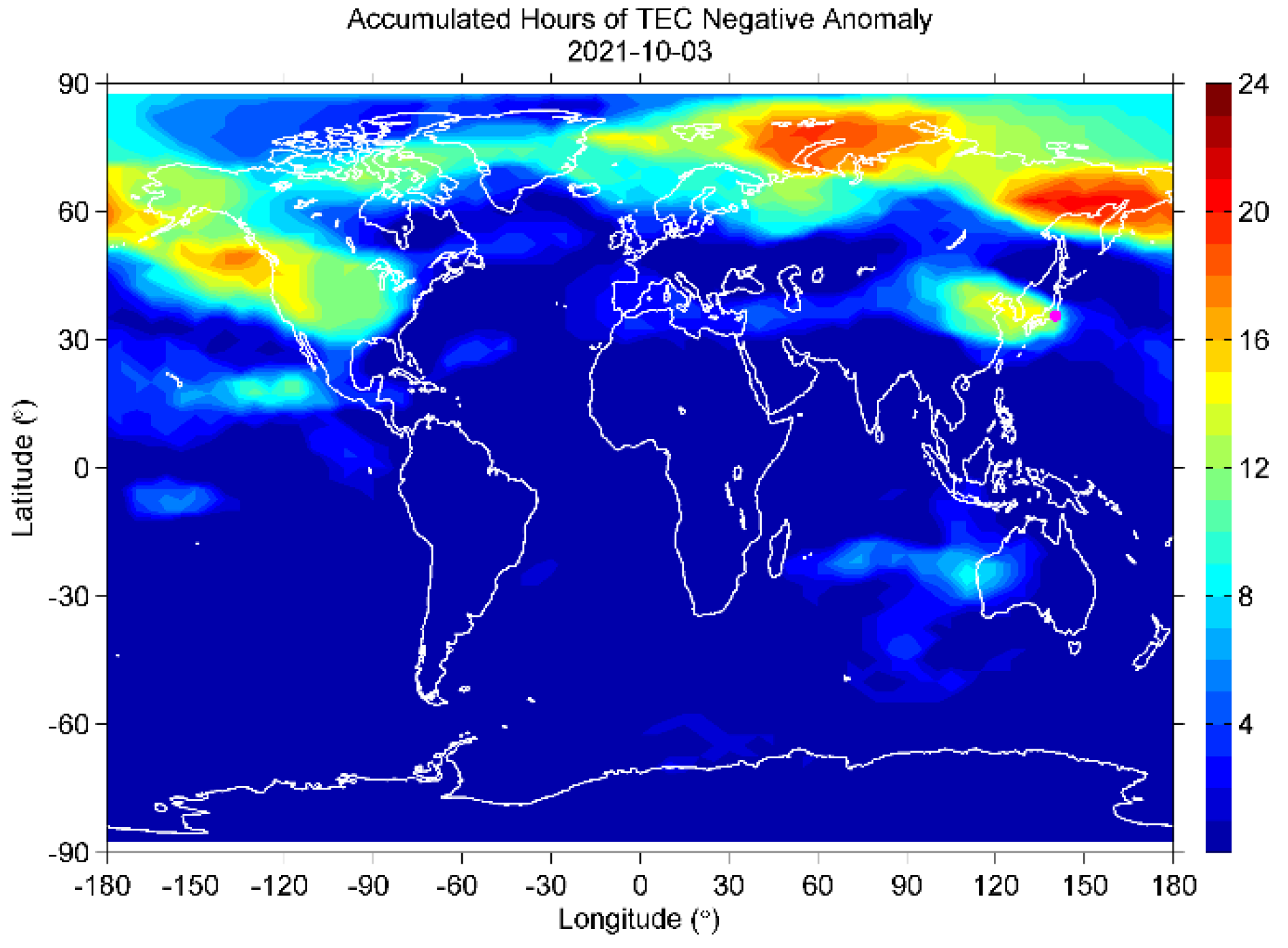
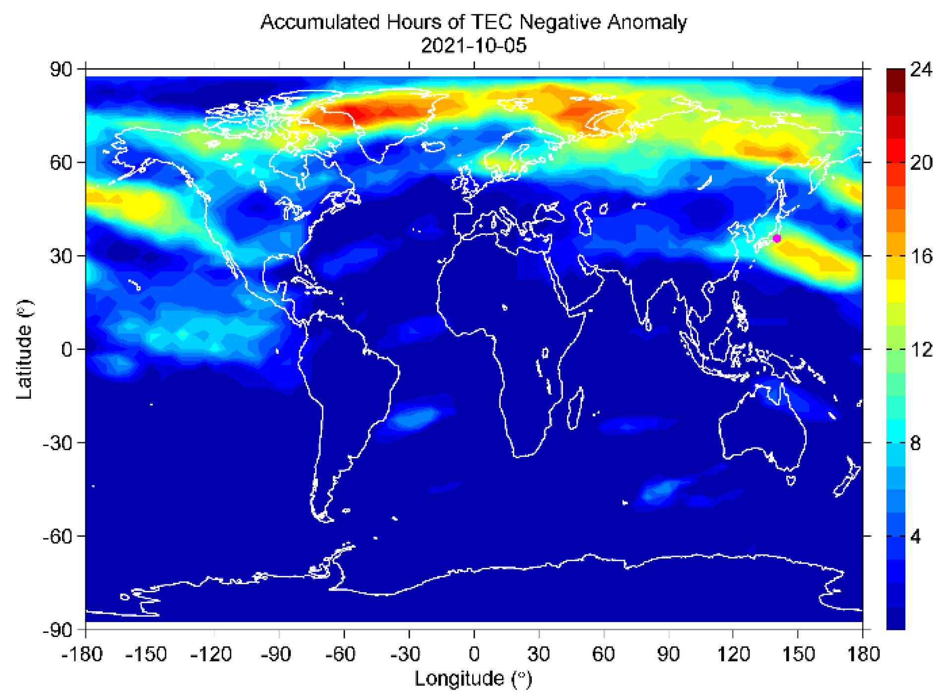
- Finally, we summarize what is happening in the upper ionosphere, such as the F region of the ionosphere [82,83]. Our extensive analyses both on the TEC and ionosonde observational data have indicated that no clear anomalies are detected during the last phase of EQ preparation, unlike the situation in the lower ionosphere. So, it seems that the initial lithospheric origin of the LAIC process is not strong enough to reach the upper F region of the ionosphere.
5. Conclusions
Author Contributions
Funding
Informed Consent Statement
Data Availability Statement
Acknowledgments
Conflicts of Interest
References
- Hayakawa, M. Earthquake Prediction Studies in Japan. In Pre-Earthquake Processes: A Multidisciplinary Approach to Earthquake Prediction Studies; Ouzounov, D., Pulinets, S., Hattori, K., Taylor, P., Eds.; AGU Monograph 234; Wiley: Hoboken, NJ, USA, 2018; pp. 7–18. [Google Scholar]
- Wikipedia. 1923 Great Kantō Earthquake. Available online: https://:en.wikipedia.org/wiki1923_kanto_earthquake (accessed on 15 December 2021).
- Pulinets, S.A.; Boyarchuk, K. Ionospheric Precursors of Earthquakes; Springer: Berlin, Germany, 2004; 315p. [Google Scholar]
- Molchanov, O.A.; Hayakawa, M. Seismo Electromagnetics and Related Phenomena: History and Latest Results; Terrapub: Tokyo, Japan, 2008; 189p. [Google Scholar]
- Hayakawa, M. Earthquake Prediction with Radio Techniques; John Wiley and Sons: Singapore, 2015; 294p. [Google Scholar]
- Ouzounov, D.; Pulinets, S.; Hattori, K.; Taylor, P. (Eds.) Pre-Earthquake Processes: A Multidisciplinary Approach to Earthquake Prediction Studies; AGU Geophysical Monograph 234; Wiley: Hoboken, NJ, USA, 2018; 365p. [Google Scholar]
- Hayakawa, M. (Ed.) Earthquake Prediction Studies: Seismo Electromagnetics; Terrapub: Tokyo, Japan, 2013; 168p. [Google Scholar]
- Pulinets, S.A.; Ouzounov, D. The Probability of Earthquake Prediction: Learning from Nature; IOP (Institute of Physics) Publishing: Bristol, UK, 2018; 168p. [Google Scholar]
- Parrot, M. Anomalous Seismic Phenomena: View from space. In Electromagnetic Phenomena Associated with Earthquakes; Hayakawa, M., Ed.; Transworld Research Network: Trivandrum, India, 2009; pp. 205–233. [Google Scholar]
- Tronin, A.A.; Hayakawa, M.; Molchanov, O.A. Thermal IR satellite data application for earthquake research in Japan and China. J. Geodyn. 2002, 33, 519–534. [Google Scholar] [CrossRef]
- Tramutoli, V.; Cuomo, V.; Filizzola, C.; Pergola, N.; Pietrapertosa, C. Assesing the potential of thermal infrared satellite surveys for monitoring seismically active areas: The case of Kocaeli (Izmit) earthquake, August 07, 1999. Remote Sens. Environ. 2005, 96, 409–426. [Google Scholar] [CrossRef]
- Ouzounov, D.; Pulinets, S.; Davidenko, D.; Rozhnoi, A.; Solovieva, M.; Fedun, V.; Dwivedi, B.N.; Rybin, A.; Kafatos, M.; Taylor, P. Transient effects in atmosphere and ionosphere preceding the 2015 M7.8 and M7.3 Gorkha-Nepal earthquakes. Front. Earth Sci. 2021, 9, 757358. [Google Scholar] [CrossRef]
- Sasmal, S.; Chowdhury, S.; Kundu, S.; Politis, D.Z.; Potirakis, S.M.; Balasis, G.; Hayakawa, M.; Chakrabarti, S.K. Pre-seismic irregularities during the 2020 Samos (Greece) earthquake (M = 6.9) as investigated from multi-parameter approach by ground and space-based techniques. Atmosphere 2021, 12, 1059. [Google Scholar] [CrossRef]
- Hayakawa, M.; Izutsu, J.; Schekotov, A.; Yang, S.S.; Solovieva, M.; Budilova, E. Lithosphere-atmosphere-lithosphere coupling effects based on multiparameter precursor observations for February–March 2021 earthquakes (M~7) in the offshore of Tohoku area of Japan. Geosciences 2021, 11, 481. [Google Scholar] [CrossRef]
- Freund, F.T. Earthquake forewarning—A multidisciplinary challenge from the ground up to space. Acta Geophys. 2013, 61, 775–807. [Google Scholar] [CrossRef]
- Sorokin, V.M.; Chmyrev, V.M.; Hayakawa, M. A review on electrodynamic influence of atmospheric processes to the ionosphere. Open J. Earthq. Res. 2020, 9, 113–141. [Google Scholar] [CrossRef]
- Sorokin, V.V.; Chmyrev, V.; Hayakawa, M. Electrodynamic Coupling of Lithosphere-Atmosphere-Ionosphere of the Earth; NOVA Science Pub. Inc.: New York, NY, USA, 2015; 355p. [Google Scholar]
- Pulinets, S.A.; Ouzounov, D.; Karelin, A.V.; Boyarchuk, K.A.; Pokhmelnykh, L.A. The physical nature of thermal anomalies observed before strong earthquakes. Phys. Chem. Earth 2006, 31, 143–153. [Google Scholar] [CrossRef]
- Pulinets, S.; Ouzounov, D. Lithosphere-atmosphere-ionosphere coupling (LAIC) model—A unified concept for earthquake precursors validation. J. Asian Earth Sci. 2011, 41, 371–382. [Google Scholar] [CrossRef]
- Hayakawa, M.; Kasahara, Y.; Nakamura, T.; Hobara, Y.; Rozhnoi, A.; Solovieva, M.; Molchanov, O.A.; Korepanov, K. Atmospheric gravity waves as a possible candidate for seismo-ionospheric perturbations. J. Atmos. Electr. 2011, 31, 129–140. [Google Scholar] [CrossRef]
- Korepanov, V.; Hayakawa, M.; Yampolski, Y.; Lizunov, G. AGW as a seismo-ionospheric coupling responsible agent. Phys. Chem. Earth 2009, 34, 485–495. [Google Scholar] [CrossRef]
- Lizunov, G.; Skorokhod, T.; Hayakawa, M.; Korepanov, V. Formation of ionospheric precursors of earthquakes—Probable mechanism and its substantiation. Open J. Earthq. Res. 2020, 9, 142. [Google Scholar] [CrossRef]
- Yang, S.S.; Asano, T.; Hayakawa, M. Abnormal gravity wave activity in the stratosphere prior to the 2016 Kumamoto earthquakes. J. Geophys. Res. Space Phys. 2019, 124, 1410–1425. [Google Scholar] [CrossRef]
- Yang, S.S.; Hayakawa, M. Gravity wave activity in the stratosphere before the 2011 Tohoku earthquake as the mechanism of lithosphere-atmosphere-ionosphere coupling. Entropy 2020, 22, 110. [Google Scholar] [CrossRef] [PubMed]
- Dobrovolsky, I.R.; Zubrov, S.I.; Myachkin, V.I. Estimation of the size of earthquake preparation zone. Pure Appl. Geophys. 1979, 117, 1025–1044. [Google Scholar] [CrossRef]
- Hayakawa, M.; Kawate, R.; Molchanov, O.A.; Yumoto, K. Results of ultra-low-frequency magnetic field measurements during the Guam earthquake of 8 August 1993. Geophys. Res. Lett. 1996, 23, 241–244. [Google Scholar] [CrossRef]
- Currie, J.L.; Waters, C.L. On the use of geomagnetic indices and ULF waves for earthquake precursor signatures. J. Geophys. Res. Space Phys. 2014, 119, 992–1003. [Google Scholar] [CrossRef]
- Guiliani, G.G.; Giuliani, R.; Totani, G.; Eusani, G.; Totani, F. Radon Observations by Gamma Detectors “PM4 and PM2” during the Seismi Period (January–April 2009) in A’Aquila Basin; AGU Fall meeting, U14A-03; American Geophysical Union: Washington, DC, USA, 2009. [Google Scholar]
- Kuntoro, Y.; Setiwan, H.L.; Wijayanti, T.; Haerundin, N. The Correlation between Radon Emission Concentration and Subsurface Geological Condition; IOP Conference Series: Earth and Environmental Science; IOP Publishing Ltd.: Bristol, UK, 2018; Volume 132. [Google Scholar] [CrossRef]
- Fu, C.C.; Wang, P.K.; Lee, L.C.; Lin, C.H.; Chang, W.Y.; Giuliani, G.; Ouzounov, D. Temporal variation of gamma ray as a possible precursor of earthquake in the longitudinal valley of eastern Taiwan. J. Asian Earth Sci. 2015, 114, 362–372. [Google Scholar] [CrossRef]
- Schekotov, A.; Hayakawa, M. Seismo-meteo-electromagnetic phenomena observed during a 5-year interval around the 2011 Tohoku earthquake. Phys. Chem. Earth 2015, 85, 167–173. [Google Scholar] [CrossRef]
- Schekotov, A.Y.; Molchanov, O.A.; Hayakawa, M.; Fedorov, E.N.; Chebrov, V.N.; Sinitsin, V.I.; Gordeev, E.F.; Belyaev, G.G.; Yagova, N.V. ULF/ELF magnetic field variation from atmosphere by seismicity. Radio Sci. 2007, 42, RS6S90. [Google Scholar] [CrossRef]
- Schekotov, A.; Fedorov, E.; Molchanov, O.A.; Hayakawa, M. Low frequency electromagnetic precursors as a prospect for earthquake prediction. In Earthquake Prediction Studies: Seismo Electromagnetics; Hayakawa, M., Ed.; Terrapub: Tokyo, Japan, 2013; pp. 81–99. [Google Scholar]
- Hayakawa, M.; Schekotov, A.; Izutsu, J.; Nickolaenko, A.P. Seismogenic effects in ULF/ELF/VLF electromagnetic waves. Int. J. Electron. Appl. Res. 2019, 6, 1–86. [Google Scholar] [CrossRef]
- Schekotov, A.; Chebrov, D.; Hayakawa, M.; Belyaev, G.; Berseneva, N. Short-term earthquake prediction at Kamchatka using low-frequency magnetic field. Nat. Hazards 2020, 100, 735–755. [Google Scholar] [CrossRef]
- Ohta, K.; Izutsu, J.; Schekotov, A.; Hayakawa, M. The ULF/ELF electromagnetic radiation before the 11 March 2011 Japanese earthquake. Radio Sci. 2013, 48, 589–596. [Google Scholar] [CrossRef]
- Fowler, R.A.; Kotick, B.J.; Elliot, R.D. Polarization analysis of natural and artificially induced geomagnetic micropulsations. J. Geophys. Res. 1967, 72, 2871–2875. [Google Scholar] [CrossRef]
- Herbach, H.; Bell, B.; Berrisford, P.; Hirahara, S.; Horanyi, A.; Munoz-Sabataer, J.; Nicolas, J.; Peubey, C.; Radu, R.; Schepers, D.; et al. The ERA5 global reanalysis. Q. J. R. Meteorol. Soc. 2020, 146, 1999–2049. [Google Scholar] [CrossRef]
- Molchanov, O.A.; Schekotov, A.Y.; Fedorov, E.N.; Belyaev, G.G.; Gordeev, E.E. Preseismic ULF electromagnetic effect from observation at Kamchatka. Nat. Hazards Earth Syst. Sci. 2003, 3, 203–209. [Google Scholar] [CrossRef]
- Molchanov, O.A.; Schekotov, A.Y.; Fedorov, E.; Belyaev, G.G.; Gordeev, E.E. Preseismic ULF electromagnetic effect and possible interpretation. Ann. Geophys. 2004, 47, 119–131. [Google Scholar]
- Schekotov, A.; Molchanov, O.; Hattori, K.; Fedorov, E.; Gladyshev, V.A.; Belyaev, G.G.; Chebrov, V.; Sinitsin, V.; Gordeev, E.; Hayakawa, M. Seismo-ionospheric depression of the ULF geomagnetic fluctuations at Kamchatka and Japan. Phys. Chem. Earth 2006, 31, 313–318. [Google Scholar] [CrossRef]
- Hayakawa, M.; Schekotov, A.; Fedorov, E.; Hobara, Y. On the ultra-low-frequency magnetic field depression for three huge oceanic earthquakes in Japan and in the Kurile islands. Earth Sci. Res. 2013, 2, 33. [Google Scholar] [CrossRef][Green Version]
- Kikuchi, T.; Evans, D.S. Quantitative study of substorm-associated VLF phase anomalies and precipitating energetic electrons on November 13, 1979. J. Geophys. Res. Space Phys. 1983, 88, 871–880. [Google Scholar] [CrossRef]
- Peter, W.B.; Chevalier, M.W.; Inan, U.S. Perturbations of midlatitude subionospheric VLF signals associated with lower ionospheric disturbances during major geomagnetic storms. J. Geophys. Res. Space Phys. 2006, 111, A3. [Google Scholar] [CrossRef]
- Hayakawa, M.; Molchanov, O.A.; Ondoh, T.; Kawai, E. The precursory signature effect of the Kobe earthquake on VLF subionospheric signals. J. Commun. Res. Lab. 1996, 43, 169–180. [Google Scholar]
- Hayakawa, M.; Kasahara, Y.; Nakamura, T.; Muto, F.; Horie, T.; Maekawa, S.; Hobara, Y.; Rozhnoi, A.A.; Solovieva, M.; Molchanov, O.A. A statistical study on the correlation between lower ionospheric perturbations as seen by subionospheric VLF/LF propagation and earthquakes. J. Geophys. Res. 2010, 115, A09305. [Google Scholar] [CrossRef]
- Molchanov, O.A.; Hayakawa, M. Subionospheric VLF signal perturbations possibly related to earthquakes. J. Geophys. Res. 1998, 103, 17489–17504. [Google Scholar] [CrossRef]
- Biagi, P.F.; Ermini, A. Geochemical and VLF-LF radio precursors of strong earthquakes. In Earthquake Prediction Studies: Seismo Electromagnetics; Hayakawa, M., Ed.; Terrapub: Tokyo, Japan, 2013; pp. 153–168. [Google Scholar]
- Rozhnoi, A.; Solovieva, M.; Molchanov, O.A.; Hayakawa, M. Middle latitude LF (40 kHz) phase variations associated with earthquakes for quiet and disturbed geomagnetic conditions. Phys. Chem. Earth 2004, 29, 589–598. [Google Scholar] [CrossRef]
- Rozhnoi, A.; Solovieva, M.; Hayakawa, M. VLF/LF signals method for searching for electromagnetic earthquake precursors. In Earthquake Prediction Studies: Seismo Electromagnetics; Hayakawa, M., Ed.; Terrapub: Tokyo, Japan, 2013; pp. 31–48. ISBN 978-4-88704-163-9. [Google Scholar]
- Maekawa, S.; Horie, T.; Yamauchi, T.; Sawaya, T.; Ishikawa, M.; Hayakawa, M.; Sasaki, H. A statistical study on the effect of earthquakes on the ionosphere, as based on the subionospheric LF of propagation data in Japan. Ann. Geophys. 2006, 24, 2219–2225. [Google Scholar] [CrossRef]
- Ray, S.; Chakrabarti, S.K.; Mondal, S.M.; Sasmal, S. Ionospheric anomaly due to seismic activities III: Correlation between nighttime VLF amplitude fluctuations and effective magnitudes in Indian sub-continent. Nat. Hazards Earth Syst. Sci. 2011, 11, 2699–2704. [Google Scholar] [CrossRef]
- Hayakawa, M.; Asano, T.; Rozhnoi, A.; Solovieva, M. Very-low and low-frequency sounding of ionospheric perturbations and possible association with earthquakes. In Pre-Earthquake Processes: A Multidisciplinary Approach to Earthquake Prediction Studies; Ouzounov, D., Pulinets, S., Hattori, K., Taylor, P., Eds.; AGU monograph; Wiley: Hoboken, NJ, USA, 2018; pp. 277–304. [Google Scholar]
- Pal, S.; Hobara, Y.; Chakrabarti, S.K.; Schnor, P.W. Effects of the major sudden stratospheric warming events of 2009 on the subionospheric very low frequency/low frequency radio signals. J. Geophys. Res. Space Phys. 2017, 122, 7555–7566. [Google Scholar] [CrossRef]
- Liu, J.Y.; Chen, Y.I.; Chuo, Y.J.; Chen, C.S. A statistical investigation of pre-earthquake ionospheric anomaly. J. Geophys. Res. 2006, 111, A05304. [Google Scholar] [CrossRef]
- Le, H.; Liu, J.Y.; Liu, L. A statistical analysis of ionospheric anomalies before 736 M 6.0+ earthquakes during 2002–2010. J. Geophys. Res. Space Phys. 2011, 116, A02303. [Google Scholar] [CrossRef]
- Schaer, S. Mapping and Predicting the Earth’s Ionosphere Using the Global Positioning System. Ph.D. Thesis, Astronomical Institute, University of Berne, Berne, Switzerland, 1999. [Google Scholar]
- Kopytenko, Y.A.; Matiashvily, T.G.; Voronov, P.M.; Kopytenko, E.A.; Molchanov, O.A. Detection of ULF emissions connected with the Spitak earthquake and its aftershock activity based on geomagnetic pulsations data at Dusheti and Vardziya observatories. Phys. Earth Planet. Inter. 1990, 77, 85–95. [Google Scholar] [CrossRef]
- Molchanov, O.A.; Kopytenko, Y.A.; Voronov, P.M.; Kopytenko, E.A.; Matiashvily, T.G.; Fraser-Smith, A.C.; Bernardi, A. Results of ULF magnetic field measurements near the epicenters of the Spitac (Ms = 6.9) and Loma Prieta (Ms = 7.1) earthquakes: Comparative analysis. Geophys. Res. Lett. 1992, 19, 1495–1498. [Google Scholar] [CrossRef]
- Fraser-Smith, A.C.; Bernardi, A.; McGill, P.R.; Ladd, M.E.; Helliwell, R.A.; Villard, O.G., Jr. Low-frequency magnetic field measurements near the epicenter of the Ms 7.1 Loma Prieta earthquake. J. Geophys. Res. 1990, 17, 1465–1468. [Google Scholar]
- Hayakawa, M.; Kawate, R.; Molchanov, O.A. Ultra-low-frequency signatures of the Guam earthquake of 8 August 1993 and its implications. J. Atmos. Electr. 1996, 16, 193–198. [Google Scholar]
- Mizutani, H.; Ishido, T.; Yokokura, T.; Ohnishi, S. Electrokinetic phenomena associated with earthquakes. Geophys. Res. Lett. 1976, 3, 365–368. [Google Scholar] [CrossRef]
- Molchanov, M.; Hayakawa, M. Generation of ULF electromagnetic emissions by microfracturing. Geophys. Res. Lett. 1995, 22, 3091–3094. [Google Scholar] [CrossRef]
- Tzanis, A.; Vallianatos, F. A physical model of electric earthquake precursors due to crack propagation and the motion of charged edge dislocations. In Seismo Electromagnetics: Lithosphere-Atmosphere-Ionosphere Coupling; Hayakawa, M., Molchanov, O.A., Eds.; Terrapub: Tokyo, Japan, 2002; pp. 117–130. [Google Scholar]
- Eftaxias, K.; Potirakis, S.M.; Contoyiannis, Y. Four-stage model of earthquake generation in terms of fracture-induced electromagnetic emission: A review. In Complexity of Seismic Time Series; Chelidze, T., Vallianatos, F., Teleska, L., Eds.; Elsevier: Amsterdam, The Netherlands, 2018; pp. 437–502. [Google Scholar]
- Varotsos, P.; Sarlis, N.; Skordas, E.S. Phenomena preceding major earthquakes interconnected through physical model. Ann. Geophys. 2019, 37, 315–324. [Google Scholar] [CrossRef]
- Potirakis, S.M.; Contoyiannis, Y.; Koulouras, G.; Nomicos, C. Recent field observations indicating an earth system in critical condition before the occurrence of a significant earthquake. IEEE Geosci. Remote Sens. Lett. 2015, 12, 631–635. [Google Scholar] [CrossRef]
- Potirakis, S.M.; Schekotov, A.; Asano, T.; Hayakawa, M. Natural time analysis on the ultra-low frequency magnetic field variations prior to the 2016 Kumamoto (Japan) earthquakes. J. Asian Earth Sci. 2018, 154, 419–427. [Google Scholar] [CrossRef]
- Potirakis, S.M.; Contoyiannis, Y.; Schekotov, A.; Eftaxias, K.; Hayakawa, M. Evidence of critical dynamics in various electromagnetic precursors. Eur. Phys. J. Spec. Top. 2021, 230, 151–177. [Google Scholar] [CrossRef]
- Hattori, K. ULF geomagnetic changes associated with large earthquakes. Terr. Atmos. Ocean. Sci. 2004, 15, 329–360. [Google Scholar] [CrossRef]
- Han, P.; Hattori, K.; Hirokawa, M.; Zhuang, J.; Chen, C.H.; Febriani, F.; Yamaguchi, H.; Yoshino, C.; Liu, J.Y.; Yoshida, S. Statistical analysis of ULF seismomagnetic phenomena at Kakioka, Japan, during 2001–2010. J. Geophys. Res. Space Phys. 2014, 119, 4998–5011. [Google Scholar] [CrossRef]
- Kamiyama, M.; Sugito, M.; Kuse, M.; Schekotov, A.; Hayakawa, M. On the precursors to the 2011 Tohoku earthquake: Crustal movements and electromagnetic signatures. Geomat. Nat. Hazards Risk 2014, 7, 471–492. [Google Scholar] [CrossRef]
- Yang, S.S.; Potirakis, S.M.; Sasmal, S.; Hayakawa, M. Natural time analysis of Global Navigation Satellite System surface deformation: The case of the 2016 Kumamoto earthquakes. Entropy 2020, 22, 674. [Google Scholar] [CrossRef]
- Bedford, J.R.; Moreno, M.; Deng, Z.; Oncken, O.; Schurr, B.; John, T.; Baez, T.C.; Bevis, M. Months-long thousand-kilometre-scale wobbling before great subduction earthquakes. Nature 2020, 580, 628–639. [Google Scholar] [CrossRef]
- Chen, C.H.; Lin, L.C.; Yeh, T.K.; Wen, S.; Yu, H.; Yu, C.; Gao, Y.; Han, P.; Sun, Y.Y.; Liu, J.Y.; et al. Determination of epicenters before earthquakes utilizing far seismic and GNSS data: Insights from ground vibrations. Remote Sens. 2020, 12, 3252. [Google Scholar] [CrossRef]
- Cervone, G.; Maekawa, S.; Singh, R.P.; Hayakawa, M.; Katafos, M.; Shvets, A. Surface heat flux and nighttime LF anomalies prior to the Mw = 8.3 Tokai-oki earthquake. Nat. Hazards Earth Syst. Sci. 2006, 6, 109–114. [Google Scholar] [CrossRef]
- Gosh, S.; Chowdhury, S.; Kundu, S.; Sasmal, S.; Politis, D.; Potirakis, S.; Hayakawa, M.; Chakraborti, S.; Chakrabarti, S.K. Unusual surface latent heat flux variations and their critical dynamics revealed before strong earthquakes. Entropy 2022, 24, 23. [Google Scholar] [CrossRef]
- Fidani, C.; Orsini, M.; Iezzi, G.; Vicentini, N.; Stoppa, F. Electric and magnetic recordings by Cieti CIEN station during the intense 2016–2017 seismic swarms in Central Italy. Front. Earth Sci. 2020, 8, 536332. [Google Scholar] [CrossRef]
- Straser, V.; Cataldi, G.; Cataldi, D. SELF and VLF electromagnetic signal variations that preceded the Central Italy earthquake on August 24, 2016. New Concepts Glob. Tecton. J. 2016, 4, 473–477. [Google Scholar]
- Schekotov, A.; Hayakawa, M.; Potirakis, S.M. Does air ionization by radon cause low-frequency earthquake precursor? Nat. Hazards 2021, 106, 701–714. [Google Scholar] [CrossRef]
- Kundu, S.; Chowdhury, S.; Gosh, S.; Sasmal, S.; Politis, D.; Potirakis, S.M.; Yang, S.S.; Chakrabarti, S.K.; Hayakawa, M. Seismogenic anomalies in Atmospheric Gravity Waves observed by SABER/TIMED satellite during large earthquakes. J. Sens. 2022, 2022, 3201104. [Google Scholar] [CrossRef]
- Picozza, P.; Conti, L.; Sotgiu, A. Looking for earthquake precursors from space. Front. Earth Sci. 2021, 9, 578. [Google Scholar] [CrossRef]
- Conti, L.; Picozza, P.; Sotgiu, A. A critical review of ground-based observations of earthquake precursors. Front. Earth Sci. 2021, 9, 676766. [Google Scholar] [CrossRef]


| DATE | LAT | LNG | MAG | DIST | DEP |
|---|---|---|---|---|---|
| 3 August 2021 | 36.0981 | 142.1045 | 5.8 | 217 | 27 |
| 13 September 2021 | 32.4784 | 137.8572 | 5.8 | 397 | 370 |
| 29 September 2021 | 38.8937 | 135.4444 | 6.1 | 521 | 364 |
| 5 October 2021 | 40.0529 | 142.141 | 5.7 | 529 | 55 |
| 7 October 2021 | 35.5778 | 140.0664 | 5.9 | 31 | 62 |
| 29 November 2021 | 31.1809 | 142.4851 | 6.3 | 562 | 6 |
| 29 November 2021 | 31.1 | 142.8 | 6.6 | 584 | 10 |
| Region | Phenomenon | Anomaly and Trend |
|---|---|---|
| Lithosphere | ULF lithospheric radiation | Nil |
| Lower Atmosphere |
| Likely precursor 10 September ~10 October (−30 days ~+a few days) Clear precursor − one week ~+one week |
| Stratosphere | AGW | Nil |
| Ionosphere (lower) |
| Obvious precursor − 2 days Obvious precursor − 2 days, +1 day |
| Ionosphere (upper) |
| Nil Nil |
Publisher’s Note: MDPI stays neutral with regard to jurisdictional claims in published maps and institutional affiliations. |
© 2022 by the authors. Licensee MDPI, Basel, Switzerland. This article is an open access article distributed under the terms and conditions of the Creative Commons Attribution (CC BY) license (https://creativecommons.org/licenses/by/4.0/).
Share and Cite
Hayakawa, M.; Schekotov, A.; Izutsu, J.; Yang, S.-S.; Solovieva, M.; Hobara, Y. Multi-Parameter Observations of Seismogenic Phenomena Related to the Tokyo Earthquake (M = 5.9) on 7 October 2021. Geosciences 2022, 12, 265. https://doi.org/10.3390/geosciences12070265
Hayakawa M, Schekotov A, Izutsu J, Yang S-S, Solovieva M, Hobara Y. Multi-Parameter Observations of Seismogenic Phenomena Related to the Tokyo Earthquake (M = 5.9) on 7 October 2021. Geosciences. 2022; 12(7):265. https://doi.org/10.3390/geosciences12070265
Chicago/Turabian StyleHayakawa, Masashi, Alexander Schekotov, Jun Izutsu, Shih-Sian Yang, Maria Solovieva, and Yasuhide Hobara. 2022. "Multi-Parameter Observations of Seismogenic Phenomena Related to the Tokyo Earthquake (M = 5.9) on 7 October 2021" Geosciences 12, no. 7: 265. https://doi.org/10.3390/geosciences12070265
APA StyleHayakawa, M., Schekotov, A., Izutsu, J., Yang, S.-S., Solovieva, M., & Hobara, Y. (2022). Multi-Parameter Observations of Seismogenic Phenomena Related to the Tokyo Earthquake (M = 5.9) on 7 October 2021. Geosciences, 12(7), 265. https://doi.org/10.3390/geosciences12070265