Analysis of HVSR Data Using a Modified Centroid-Based Algorithm for Near-Surface Geological Reconstruction

Abstract

Recently, the use of microtremor techniques for subsoil investigation has increased significantly. The HVSR (Horizontal to Vertical Spectral Ratio) technique allows, in many cases, to obtain a seismo-stratigraphic reconstruction of the subsoil and to identify areas with similar seismic behavior. However, the stratigraphic interpretation of the HVSR peaks still remains a subjective choice and linked to a priori information. A non-hierarchical centroid-based algorithm was modified to group HVSR peaks of different measurements that can be attributed to the same generating seismic discontinuity. Some tests performed have shown that the proposed algorithm produces valid results even in the absence of a priori information to evaluate the choice of the optimal grouping. The results obtained for HVSR measurements acquired in the city of Modica (Italy) are presented. The cluster analysis of these data and the information on the lithologies outcropping in the area made it possible to reconstruct a 3D model of the main seismo-stratigraphic discontinuities.

1. Introduction

The Horizontal to Vertical Spectral Ratio (HVSR) noise method [1,2,3] is currently a very popular method in seismic microzonation studies, as it has been shown to provide coherent information on site effects, i.e., significant increases of peak amplitude of ground shaking [4,5,6,7]. In the HVSR method, environmental noise, which includes microtremors induced by wind, ocean waves, and anthropogenic activity, is recorded using triaxial broadband velocimeters that measure the vertical component and the two horizontal components (north-south and east-west) [8]. The statistical analysis of the spectral components allows one to derive the trend of the ratio of the average horizontal-to-vertical spectrum. The shape of the HVSR curve approximates the spectrum of the transfer function of the sedimentary cover with respect to the bedrock. Consequently, the resonance frequencies of the site can be obtained from this. The analysis of the peaks of the HVSR curve allows one to recognize those reasonably caused by stratigraphic discontinuities. Stratigraphic peaks can be interpreted using regression equations to estimate the sediment thickness and depth with respect to the bedrock [9]. Moreover, geographically close measurements are more likely to show similar frequency peaks if they are caused by the same stratigraphic limit. This consideration can be exploited to correlate information and build bedrock frequency and depth maps, for example [10]. The uncertainty on the sources of the HVSR peaks can be reduced with cluster analysis techniques [11] in order to distinguish between peaks mainly related to site effects and peaks mainly related to source effects. Some authors have used cluster analysis techniques to distinguish peaks caused by source effects and peaks due to site effects [7,12,13,14]. The discrimination between these two effects can allow one to select the appropriate cluster of curves linked only to the site effects and consequently to derive a more reliable average HVSR curve, better identifying all the significant peaks of the H/V spectral ratio.

Often, the HVSR curves are inverted to obtain one-dimensional models of seismic velocity and layer thickness and consequently estimate the depth of the seismic bedrock [13,15,16,17]. However, the HVSR inversion must always be constrained by detailed stratigraphic information [7,17,18,19,20,21].

Many authors have shown how the uncertainty of the solution of the inverse problem in HVSR can be limited by using data from other geophysical methods as a priori constraints [16,22,23,24,25,26,27,28]. In this regard, the shear wave velocity models obtained from Multichannel Analysis of Surface Waves (MASW) can be used as initial models for the inversion of the HVSR curve [13,29,30,31,32].

Cluster analysis can also be applied on the spatial distribution of all significant peaks observed in a set of HVSR curves to identify and group the peaks likely due to the same site effect [13,14,33] and delimit areas with the same seismic response. Although we cannot completely exclude that the peaks belonging to the same cluster are due to different structures, it is statistically plausible to consider the main clusters of HVSR peaks to define the seismic layers, each characterized by a specific range of seismic velocities, and to associate them with the known geological formations. The depth values obtained by inverting the HVSR mean curves, if related to peaks of the same cluster, can then be interpolated to reconstruct a seismic stratigraphic limit.

2. Materials and Methods

Cluster analysis is a multivariate analysis technique used in many research fields [11,34,35,36], through which it is possible to combine a set of statistical units, dividing it into some subsets, called clusters, which tend to be homogeneous within them. This grouping is based on the level of internal similarity (intra-cluster) and external dissimilarity (inter-cluster) evaluated by the values that a number of chosen parametric variables assume in each unit. Cluster analysis generally does not foresee any interpretative model but is based only on statistical considerations [37]. At the end of the procedure, the objects inside the clusters are close to each other, while the objects belonging to different clusters are distant from each other. The parametric distance is quantified by measures of similarity/dissimilarity between defined statistical units.

Many clustering algorithms have been proposed [38]; they can be classified into two main classes: Hierarchical Clustering (HC) and Non-Hierarchical Clustering (NHC). In HC the objects are progressively grouped (agglomerative hierarchical clustering) or divided (divisive hierarchical clustering) into clusters, evaluating the proximity between the objects. In HC, it is not necessary to define the number of clusters in advance. At the end of the procedure, similar clusters are grouped and arranged hierarchically according to a dendrogram, which allows you to get an idea of the adequate number of clusters in which the data can be grouped.

On the other hand, NHC algorithms do not follow a tree structure and involve the formation of new clusters by joining or splitting the clusters. These techniques group the data in order to maximize or minimize some evaluation criteria. The number of clusters, the presence of outliers, and the parameters used for distance measurements primarily affect the results of the cluster analysis.

Different clustering strategies often lead to dissimilar results [39,40,41]. In any case, to assess the performance of the clustering procedure, it is necessary to evaluate the stability and the objectivity of the partition results [42]. Generally speaking, if we are looking for groups of statistical units characterized by a high internal consistency, non-hierarchical techniques are more effective than hierarchical ones.

A multiparametric clustering procedure is described here, with the aim of grouping the H/V peaks attributable to the same origin (stratigraphic, tectonic, topographic, anthropogenic, or other sources). This clustering is carried out in order to delineate the areas within which it is possible to hypothesize a continuous trend of the parameters used to describe the subsoil and of the seismic behavior of the subsoil. Many studies [13,14,17,21,24,26] demonstrated that the hypotheses on the cause of HVSR peaks are fundamental to extract reliable information on the subsoil from these data.

The parameters considered for the determination of the clusters are the coordinates (x, y, z) of the measurement, the peak frequency f₀, the H/V ratio in correspondence of f₀, and the lithology emerging at the measurement point. In particular, the geological information is converted into numerical information L, assigning to the point the value of the average density of the corresponding lithology, which is directly related to its seismic behavior.

The procedure is based on the use of a non-hierarchical algorithm based on mobile centers in which the number k of clusters is not chosen a priori. In practice, the mobile centers algorithm is repeatedly applied to the set of n data using different values of k (in our tests, k varying from 2 to 7). The choice of the optimal value of k is determined a posteriori, based on the analysis of the values assumed by the deviance within the individual clusters and by that between the clusters.

The initialization of the non-hierarchical algorithm requires the choice of the number of k classes to which to aggregate the units and the random choice of the k elements e₁⁰, e₂⁰, …, e_k⁰, which represent the provisional nuclei of the k classes. After calculating the distances of each element from the k nuclei and assigning each of these to the group represented by the closest nucleus, we identify a first partition of the set E into k classes C₁⁰, C₂⁰, …, C_k⁰. However, our approach provides that the algorithm is not linked to the initial choice of the number k of clusters. The algorithm is repeatedly applied to the set of n data by varying k from a value k_min to a value k_max (for example, from 2 to 7).

Centroid-based algorithms generally require that the number of clusters k and the starting coordinates of the centroids are specified in advance. This aspect is considered one of the major drawbacks of these algorithms because an inappropriate choice in this regard can produce poor results. That is why it is important to run diagnostic checks to determine the number of clusters in the dataset. In particular, it is known that the parameter k is difficult to choose when it is not given by external constraints.

The proposed algorithm starts with the first iteration by choosing, independently, the coordinates of the first centroids. In particular, the parametric coordinates regarding the spatial position, the H/V amplitude, and the lithology are chosen the same for all the centroids, corresponding to their average value among all the units.

The differentiation on the coordinates of the initial centroids is limited only to the peak frequency f₀, partitioning the range between the minimum and maximum frequency of all the data in a number of frequency intervals equal to the number of partitions chosen, in logarithmic scale.

The first aggregation is performed only based on the peak frequencies and the parametric coordinates of the cluster centroids are subsequently calculated to start a new iteration. In this way, the new nuclei e₁¹, e₂¹, …, e_k¹ of the classes are defined, identified in the centers of the classes themselves. After calculating the distances of each element from the new nuclei and assigning each of these to the group represented by the closest nucleus, we identify a second partition of the set E into k classes C₁¹, C₂¹, …, C_k¹. This sequence is repeated until two successive iterations define the same partition, which is then considered final.

The Euclidean distance of each element from the initial nuclei and from the nuclei obtained after each iteration is calculated as the weighted sum of the distances of all the variables considered (position, frequency, amplitude, and lithology):

$$D={\left[a\left(d{x}^2+d{y}^2+d{z}^2\right)+b\left(d{f}^2\right)+c\left(d{A}^2\right)+d\left(d{L}^2\right)\right]}^{\frac{1}{2}},$$

(1)

where dx, dy, dz, df, dA, and dL are the differences between the parametric coordinates UTMX, UTMY, elevation, frequency, amplitude, and lithology, respectively, and a, b, c, and d are the weights. The information on the emerging lithostratigraphic unit is converted into numerical information using nearby numbers for seismically similar lithologies and distant numbers for different lithologies.

The optimization of cluster analysis, i.e., the choice of the optimal number of clusters and the optimal set of weights, is made through a joint analysis of the trend of the deviance within the individual groups DEV_IN and the deviance between groups DEV_OUT:

$$DE{V}_{IN}={\displaystyle \sum }_{k=1}^g{\displaystyle \sum }_{s=1}^p{\displaystyle \sum }_{i=1}^{n_1}{\left(x_{i,s}-x_{s,k}\right)}^2$$

(2)

$$DE{V}_{OUT}={\displaystyle \sum }_{s=1}^p{\displaystyle \sum }_{k=1}^g{\left(x_{s,k}-x_s\right)}^2{n}_k$$

(3)

where g is the maximum number of clusters, p is the total number of variables considered, n is the number of data for each variable, x_i,s is the i-th datum relating to the s-th variable, and x_s,k is the mean of the s-th variable with reference to the k-th group.

Considering that the total deviance DEV_T is given by:

$$DE{V}_T={\displaystyle \sum }_{s=1}^p{\displaystyle \sum }_{i=1}^n{\left(x_{i,s}-x_s\right)}^2$$

(4)

we have:

$$DE{V}_T=DE{V}_{IN}+DE{V}_{OUT}.$$

(5)

In passing from k + 1 to k groups (aggregation) DEV_IN increases while, predictably, DEV_OUT decreases.

The partition validity indicator [43] is instead provided by:

$$R^2=\frac{DE{V}_{OUT}}{DE{V}_T}$$

(6)

but fundamentally it remains a subjective choice of the operator, based on the a priori and contextual information of the data.

The algorithm was tested using a data set of 100 HVSR measurements acquired in the urban center of Modica (Italy). From the HVSR curves, the values of the peak frequencies, H/V amplitudes, as well as UTM coordinates and outcropping lithologies L were preliminarily obtained.

We considered nine sets of different weights (

Table 1. Weight sets used to calculate the Euclidean distance.

Weight Set #	Location Weight a	Frequency Weight b	Amplitude Weight c	Lithology Weight d
1	0.6	0.2	0.15	0.05
2	0.55	0.25	0.15	0.05
3	0.5	0.3	0.15	0.05
4	0.45	0.35	0.15	0.05
5	0.4	0.4	0.15	0.05
6	0.35	0.45	0.15	0.05
7	0.3	0.5	0.15	0.05
8	0.25	0.55	0.15	0.05
9	0.2	0.6	0.15	0.05

) in which the coordinates weight a increases as the weight set number increases, while the frequency weight b decreases. The amplitude weight and the lithology weight are kept constant at c = 0.15 and d = 0.05, respectively.

Figure 1 shows the histograms relating to DEV_IN (top) and the those relating to DEV_OUT (bottom) for the k clusters considered (k ranging from 2 to 7 clusters) as the weight set varies.

It should be noted that DEV_IN increases as the position weight a increases and as the frequency weight b decreases, while it decreases as the number of clusters k increases. On the other hand, the DEV_OUT has a mirror behavior, considering that DEV_T = DEV_IN + DEV_OUT.

The results of these tests prompted us to use the weight set #4 (a = 0.45, b = 0.35, c = 0.15, d = 0.05) for all subsequent analyses, considering that a lower value of the frequency weight, and greater value of the position weight, compared to those chosen, show a rapid increase in DEV_IN and decrease in DEV_OUT.

The average frequencies of the clusters, for each grouping from k = 2 to k = 7, obtained considering the weight set #4, are shown in

Table 2. Average frequencies of the clusters, for each grouping from k = 2 to k = 7, obtained considering the weight set #4.

	C1	C2	C3	C4	C5	C6	C7
k = 2	1.05 Hz	17.35 Hz
k = 3	1.05 Hz	4.27 Hz	17.35 Hz
k = 4	1.05 Hz	2.67 Hz	6.81 Hz	17.35 Hz
k = 5	1.05 Hz	2.12 Hz	4.27 Hz	8.60 Hz	17.35 Hz
k = 6	1.05 Hz	1.84 Hz	3.22 Hz	5.65 Hz	9.90 Hz	17.35 Hz
k = 7	1.05 Hz	1.67 Hz	2.67 Hz	4.27 Hz	6.81 Hz	10.87 Hz	17.35 Hz

.

The results of the proposed algorithm were compared with those obtained using as coordinates of the initial centroids those resulting from an accurate preliminary data analysis. In the absence of other information, only the information on the frequency of the H/V peaks f₀ was used for this first partition. Once the first partition was made, the distance of each point was calculated with respect to all the points within the same cluster, and the points whose minimum distance was greater than 600 m (twice the average distance between the measuring points) were discarded. This choice made it possible to calculate the initial coordinates of the centroids without the distortion in space (x, y, z) caused by isolated and distant points, although characterized by similar peak frequencies. The points left within the clusters were used to calculate the average coordinates of the centroids of each cluster to be used as input data for the nonhierarchical algorithm.

The results obtained by carrying out the preliminary analysis of the data and those obtained by applying the nonhierarchical algorithm with automatically chosen centroids are compared, for k = 5, in Figure 2 (distribution in the frequency domain) and in Figure 3 (distribution in the spatial domain).

It is highlighted how the separation of clusters in the frequency domain is clearer, leaving the algorithm free to choose the coordinates of the initial centroids rather than imposing constraints on the distance of the points in the spatial coordinate domain.

Comparing the values assumed by the parameter R² in the two different clustering procedures, we obtained R² = 0.77 for the unconstrained algorithm and R² = 0.72 for those constrained by a priori choices.

Considering that a high value of R² indicates good clustering (minimum deviance within clusters and maximum deviance between clusters), the results indicate a good partition level and then the unconstrained algorithm produces statistically better results.

The greatest differences, especially in the distribution of points in the spatial coordinate domain, are obviously evident in the second, third, and fourth clusters, which represent the groups with the greatest number of units.

In order to choose the optimal number of clusters, at least from a purely statistical point of view, it is proposed to refer to the trend of the deviance values DEV_IN, DEV_OUT, DEV_T, and, consequently, of the ratio $R^2=\frac{DE{V}_{OUT}}{DE{V}_T}$, as the number of partitions varies (Figure 4). As can be noted, although the value of R² tends to be 1 for a number of clusters equal to n, the 3-clusters grouping is the one in which R² changes the variation rate, reaching a value equal to 0.745.

Based on these considerations and in the absence of other information (for example, data on the main lithologies of the subsoil) the statistically most-valid choice will be the grouping of three clusters.

3. Results

During 2012, as part of an agreement with the Italian Civil Protection Department, a first-level seismic microzonation was performed in those municipalities in Sicily considered to be at high seismic risk. In this context, 100 HVSR measurements were performed in the inhabited center of the city of Modica. These measures, as previously mentioned, have been used to test the cluster analysis approach described in this article and, through this, to perform a seismo-stratigraphic modeling.

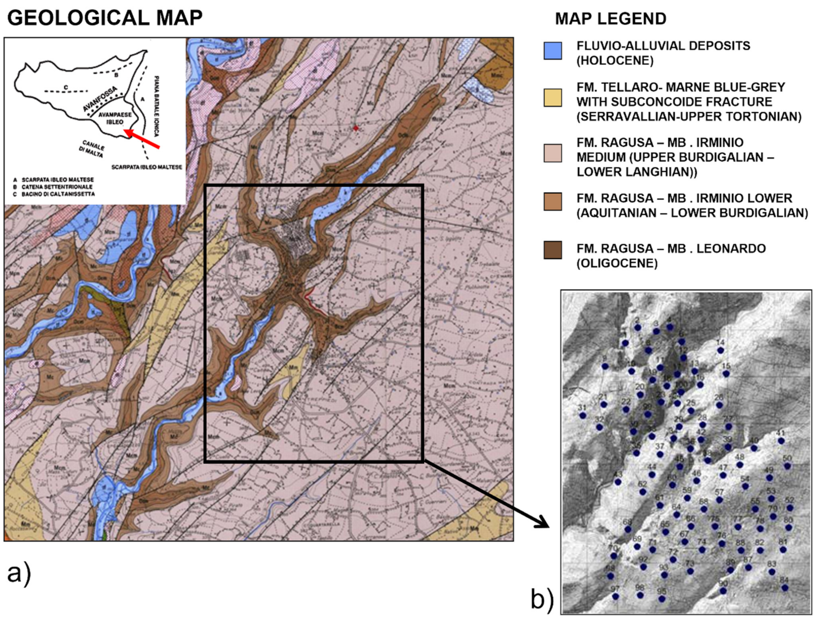
3.1. Geological Outlines

The municipal area of Modica city extends in the central sector of the Hyblean zone. The Hyblean Mountains together with the submerged zones of the Strait of Sicily constitute a sector of the African foreland that, from Southwestern Sicily, extends across the Strait of Sicily to Tunisia and Libya [44].

The geological outcrops of the territory of Modica (Figure 5) consist of mainly carbonatic-marly Oligo-Miocene successions referable to the Ragusa Formation and more marly deposits with rare intercalations of calcarenites and marly calcarenites of the Middle and Upper Miocene (Tellaro Formation). In the depressed areas of the valley floor, recent and current fluvio-alluvial deposits are also reported, mainly consisting of carbonate pebbles of variable dimensions, from centimeters to decimeters, immersed in a mostly sandy-silty matrix [45].

3.2. Application of the HVSR Technique to Microtremor Measurements

The analysis with the Nakamura method was performed on each ambient noise recording to derive the average HVSR curves. The high number of recording points served to guarantee a statistically accurate interpretation, and subsequently a sufficiently detailed reconstruction of the main seismic-stratigraphic interfaces of the subsoil.

For each measurement point, the time of each microtremor recording was 46 min and the sampling frequency was 256 Hz. Each of the 3-axial components of noise was divided into 138 time-windows of 20 s, in order to allow a more than adequate number of analysis windows, according to SESAME recommendations [46].

After detrending and smoothing the signals, the HVSR curves in frequency domain were determined and their geometric means and standard deviations were estimated. The selection of the significant noise windows was performed by applying an Agglomerative Hierarchical Clustering algorithm (AHC) [37,38], using Standard Correlation (SC_xy) defined as:

$$S{C}_{xy}={\displaystyle \sum }_{i=1}^n{x}_i\cdot y_i/\sqrt{{\displaystyle \sum }_{i=1}^n{x}_i^2\cdot {\displaystyle \sum }_{i=1}^n{y}_i^2}$$

(7)

where x_i and y_i indicate the values of the spectral ratios relating to the i-th frequency and the generic pair of analysis windows [11]. This procedure allows one to group the curves relating to each window by degrees of similarity and to distinguish and discard those curves that showed trends and peaks not referable to stratigraphic attributes.

In this way, time windows relating to transient noises or having clearly non-stratigraphic peaks were discarded. The HVSR average curves thus obtained were examined to identify the main seismo-stratigraphic peaks.

3.3. Cluster Analysis of the H/V Peaks

Finally, the method discussed in the previous paragraph was applied to the obtained dataset.

All the partitions obtained (from k = 2 to k = 7) were superimposed on the geological map shown in Figure 5 to identify correlations with geology and topography.

Not considering the small thickness of alluvial fluvial deposits, whose presence is however limited to river incisions, the absence of important tectonic discontinuities suggests the areal continuity of the aforementioned lithologies in the studied area. Consequently, the presence of only three main seismo-stratigraphic boundaries between four different lithologies (the three members of the Ragusa Fm. and the Tellaro Fm.) was hypothesized. This confirms the choice of the optimal number of clusters obtained only through the statistical evaluation of the data (Figure 4). The central frequencies of the clusters are 1.05 Hz for cluster #1, 4.27 Hz for cluster #2, and 17.35 Hz for cluster #3. The spatial distribution of these three clusters is shown in Figure 6.

3.4. Seismo-Stratigraphic Modeling

The results of some Multichannel Analysis of Surface Waves (MASW) [47] surveys were used to constrain the seismic velocities of the first layers in HVSR inversions [28,30]. These latter surveys were performed using the Dinver module of the Geopsy open source software [48], using similar starting models for each cluster.

Each individual cluster of HVSR peaks was considered to define a different seismic layer, each characterized by a specific range of seismic velocities, and to associate them with a known geological formation or member.

Figure 7a shows an example of an HVSR curve in which two peaks are visible: one belonging to cluster #1 (f₀ = 0.9 Hz) and the other belonging to cluster #3 (f₁ = 9.5 Hz). However, the curve lacks peaks belonging to cluster #2. Consequently, the obtained inverse model (Figure 7b) shows two seismo-stratigraphic boundaries at z = 124 m and z = 295 m respectively.

The layer thicknesses obtained were spatially interpolated to reconstruct the three seismo-stratigraphic surfaces. These were superimposed on the geological map (Figure 8) to highlight correlations with geology and topography. Observing the overlaps, it can be seen that the areas in which the altitude of the seismo-stratigraphic boundaries is greater than the topographic altitude (less transparent colored areas) correspond quite well with the outcrop limits of each lithology. This is a good indication of a robust interpretation. Finally, a three-dimensional representation of the seismo-stratigraphic model is shown in Figure 9.

4. Discussion

Contrary to other statistical procedures, cluster analysis is often used when there is no a priori hypothesis or in the exploratory phase of the analysis. However, the application of cluster analysis, even though it is one of the essentially exploratory methods of analysis, should be preceded and accompanied by the definition of interpretative models.

A weakness of cluster analysis is that of arriving at indeterminate solutions, subject to arbitrary decisions relating to the initial information, to the subjective interpretation of the results, and not statistically verifiable.

The proposed cluster analysis algorithm applied to the stratigraphic determination of HVSR peaks has shown excellent results, allowing the grouping of peaks attributable to the same generating seismic surfaces.

However, the tests performed have shown that the algorithm works without the need to choose the number of clusters in advance, which can be determined independently through the analysis of the R² parameter. However, although the results of the applied algorithm are similar regardless of the a priori choices, the best partition is linked to the choice of weights for calculating the distance D and to the geological and stratigraphic knowledge of the area.

The application of the proposed algorithm to the data acquired in the city of Modica made it possible to correctly identify three main clusters linked to the presence of three seismic impedance discontinuities. This procedure made it possible to reconstruct a 3D model of the subsoil that is well correlated with the geological information of the area and with the outcrop lithology.

References

1. Nakamura, Y. Method for dynamic characteristics estimation of subsurface using microtremor on the ground surface. Q. Rep. RTRI Railw. Tech. Res. Inst. 1989, 30, 25–33. [Google Scholar]
2. Nakamura, Y. Clear Identification of Fundamental Idea of Nakamura’s Technique and its Applications. In Proceedings of the 12th World Conference on Earthquake Engineering, Auckland, New Zealand, 30 January–4 February 2000; p. 2656. [Google Scholar]
3. Nakamura, Y. What Is the Nakamura Method? Seismol. Res. Lett. 2019, 90, 1437–1443. [Google Scholar] [CrossRef]
4. Lachet, C.; Bard, P.Y. Numerical and theoretical investigations on the possibilities and limitations of Nakamura’s technique. J. Phys. Earth 1994, 42, 377–397. [Google Scholar] [CrossRef]
5. Kudo, K. Practical estimates of site response. State-of-art report. In Proceedings of the 5th International Conference on Seismic Zonation, Nice, France, 17–19 October 1995. [Google Scholar]
6. Bard, P.Y. Microtremor measurements: A tool for site effect estimation? In Proceedings of the 2nd International Symposium on the Effects of Surface Geology on Seismic Motion, Yokohama, Japan, 1–3 December 1998; pp. 1251–1279. [Google Scholar]
7. Mucciarelli, M.; Gallipoli, M.R.; Arcieri, M. The stability of the horizontal-to-vertical spectral ratio of triggered noise and earthquake recordings. Bull. Seismol. Soc. Am. 2003, 93, 1407–1412. [Google Scholar] [CrossRef]
8. Bonnefoy-Claudet, S.; Cotton, F.; Bard, P.-Y. The nature of noise wavefield and its applications for site effects studies. A literature review. Earth Sci. Rev. 2006, 79, 205–227. [Google Scholar] [CrossRef]
9. Ibs-von Seht, M.; Wohlenberg, J. Microtremor measurements used to map thickness of soft sediments. Bull. Seismol. Soc. Am. 1999, 89, 250–259. [Google Scholar] [CrossRef]
10. Bignardi, S.; Yezzi, A.J.; Fiussello, S.; Comelli, A. OpenHVSR—Processing toolkit: Enhanced HVSR processing of distributed microtremor measurements and spatial variation of their informative content. Comput. Geosci. 2018, 120, 10–20. [Google Scholar] [CrossRef]
11. D’Alessandro, A.; Luzio, D.; Martorana, R.; Capizzi, P. Selection of time windows in the Horizontal to Vertical Noise Spectral Ratio by means of cluster analysis. Bull. Seismol. Soc. Am. 2016, 106, 560–574. [Google Scholar] [CrossRef]
12. Rodriguez, V.H.S.; Midorikawa, S. Applicability of the H/V spectral ratio of microtremors in assessing site effects on seismic motion. Earthq. Eng. Struct. Dyn. 2002, 31, 261–279. [Google Scholar] [CrossRef]
13. Martorana, R.; Capizzi, P.; Avellone, G.; Siragusa, R.; D’Alessandro, A.; Luzio, D. Assessment of a geological model by surface wave analyses. J. Geophys. Eng. 2017, 14, 159–172. [Google Scholar] [CrossRef] [Green Version]
14. Martorana, R.; Agate, M.; Capizzi, P.; Cavera, F.; D’Alessandro, A. Seismo-stratigraphic model of “La Bandita” area (Palermo Plain, Sicily) through HVSR inversion constrained by stratigraphic data. Ital. J. Geosci. 2018, 137, 73–86. [Google Scholar] [CrossRef]
15. Fäh, D.; Kind, F.; Giardini, D. Inversion of local S wave velocity structures from average H/V ratios, and their use for the estimation of site-effects. J. Seismol. 2003, 7, 449–467. [Google Scholar] [CrossRef]
16. Picotti, S.; Francese, R.; Giorgi, M.; Pettenati, F.; Carcione, J.M. Estimation of glaciers thicknesses and basal properties using the horizontal-to-vertical component spectral ratio (HVSR) technique from passive seismic data. J. Glaciol. 2017, 63, 229–248. [Google Scholar] [CrossRef] [Green Version]
17. Martorana, R.; Capizzi, P.; D’Alessandro, A.; Luzio, D.; Di Stefano, P.; Renda, P.; Zarcone, G. Contribution of HVSR measures for seismic microzonation studies. Ann. Geophys. 2018, 61, SE225. [Google Scholar] [CrossRef]
18. Konno, K.; Ohmachi, T. Ground-motion characteristics estimated from spectral ratio between horizontal and vertical components of microtremor. Bull. Seismol. Soc. Am. 1998, 88, 228–241. [Google Scholar] [CrossRef]
19. Parolai, S.; Bindi, D.; Augliera, P. Application of the Generalized Inversion Technique (GIT) to a microzonation study: Numerical simulations and comparison with different site-estimation techniques. Bull. Seismol. Soc. Am. 2000, 90, 286–297. [Google Scholar] [CrossRef]
20. Fäh, D.; Kind, F.; Giardini, D. A theoretical investigation of average H/V ratios. Geophys. J. Int. 2001, 145, 535–549. [Google Scholar] [CrossRef] [Green Version]
21. Bignardi, S. The uncertainty of estimating the thickness of soft sediments with the HVSR method: A computational point of view on weak lateral variations. J. Appl. Geophy. 2017, 145, 28–38. [Google Scholar] [CrossRef]
22. Scherbaum, F.; Hinzen, K.-G.; Ohrnberger, M. Determination of shallow shear-wave velocity profiles in Cologne, Germany area using ambient vibrations. Geophys. J. Int. 2003, 152, 597–612. [Google Scholar] [CrossRef] [Green Version]
23. Arai, H.; Tokimatsu, K. S-wave velocity profiling by inversion of microtremor H/V spectrum. Bull. Seismol. Soc. Am. 2004, 94, 53–63. [Google Scholar] [CrossRef] [Green Version]
24. Parolai, S.; Picozzi, M.; Richwalski, S.M.; Milkereit, C. Joint inversion of phase velocity dispersion and H/V ratio curves from seismic noise recordings using a genetic algorithm, considering higher modes. Geophys. Res. Lett. 2005, 32, L01303. [Google Scholar] [CrossRef] [Green Version]
25. Parolai, S.; Richwalski, S.M.; Milkereit, C.; Fäh, D. S-wave velocity profiles for earthquake engineering purposes for the Cologne Area (Germany). Bull. Earthq. Eng. 2006, 4, 65–94. [Google Scholar] [CrossRef]
26. Picozzi, M.; Parolai, S.; Richwalski, S.M. Joint inversion of H/V ratios and dispersion curves from seismic noise: Estimating the S-wave velocity of bedrock. Geophys. Res. Lett. 2005, 32, L11308. [Google Scholar] [CrossRef]
27. Imposa, S.; Grassi, S.; De Guidi, G.; Battaglia, F.; Lanaia, G.; Scudero, S. 3D subsoil model of the San Biagio ‘Salinelle’ mud volcanoes (Belpasso, SICILY) derived from geophysical surveys. Surv. Geophys. 2016, 37, 1117–1138. [Google Scholar] [CrossRef]
28. Imposa, S.; Grassi, S.; Fazio, F.; Rannisi, G.; Cino, P. Geophysical surveys to study a landslide body (north-eastern Sicily). Nat. Hazards 2017, 86, 327–343. [Google Scholar] [CrossRef]
29. Zor, E.; Özalaybey, S.; Karaaslan, A.; Tapirdamaz, M.C.; Özalaybey, S.Ç.; Tarancioglu, A.; Erkan, B. Shear wave velocity structure of the Izmit Bay area (Turkey) estimated from active-passive array surface wave and single-station microtremor methods. Geophys. J. Int. 2010, 182, 1603–1618. [Google Scholar] [CrossRef] [Green Version]
30. Capizzi, P.; Martorana, R. Integration of constrained electrical and seismic tomographies to study the landslide affecting the Cathedral of Agrigento. J. Geophys. Eng. 2014, 11, 045009. [Google Scholar] [CrossRef]
31. Castellaro, S. The complementarity of H/V and dispersion curves. Geophysics 2016, 81, T323–T338. [Google Scholar] [CrossRef]
32. Panzera, F.; Sicali, S.; Lombardo, G.; Imposa, S.; Gresta, S.; D’Amico, S. A microtremor survey to define the subsoil structure in a mud volcanoes area: The case study of Salinelle (Mt. Etna, Italy). Environ. Earth Sci. 2016, 75, 1140. [Google Scholar] [CrossRef]
33. Capizzi, P.; Martorana, R.; Stassi, G.; D’Alessandro, A.; Luzio, D. Centroid-based cluster analysis of HVSR data for seismic microzonation. In Proceedings of the Near Surface Geoscience 2014—20th European Meeting of Environmental and Engineering Geophysics, Athens, Greece, 14–18 September 2014. [Google Scholar] [CrossRef]
34. Hartigan, J.A. Clustering Algorithms; Wiley: New York, NY, USA, 1975. [Google Scholar]
35. Adelfio, G.; Chiodi, M.; D’Alessandro, A.; Luzio, D.; D’Anna, G.; Mangano, G. Simultaneous seismic wave clustering and registration. Comput. Geosci. 2012, 44, 60–69. [Google Scholar] [CrossRef]
36. D’Alessandro, A.; Mangano, G.; D’Anna, G.; Luzio, D. Waveforms clustering and single-station location of microearthquake multiplets recorded in the northern Sicilian offshore region. Geophys. J. Int. 2013, 194, 1789–1809. [Google Scholar] [CrossRef] [Green Version]
37. Gan, G.; Ma, C.; Wu, J. Data Clustering: Theory, Algorithms, and Applications; Cambridge University Press: Cambridge, UK, 2007; p. 184. ISBN 9780898716238. [Google Scholar]
38. Everitt, B.S.; Landau, S.; Leese, M.; Stahl, D. Cluster Analysis, 5th ed.; Wiley Series in Probability and Statistics; John Wiley & Sons, Ltd.: London, UK, 2011; p. 332, ISBN-10 0470749911, ISBN-13 978-0470749913. [Google Scholar]
39. Rand, W.M. Objective criteria for the evaluation of clustering methods. J. Am. Stat. Assoc. 1971, 66, 846–850. [Google Scholar] [CrossRef]
40. Everitt, B.S. Unresolved problems in cluster analysis. Biometrics 1979, 35, 169–181. [Google Scholar] [CrossRef]
41. Ohsumi, N. Evaluation procedure of agglomerative hierarchical clustering methods by fuzzy relations. In Data Analysis and Informatics: Proceedings of the II International Symposium on Data Analysis and Informatics, Versailles, France, 17–19 October 1979; Tomassone, R., Pagès, J.P., Lebart, L., Diday, E., Eds.; North Holland Publishing Company: Amsterdam, The Netherlands, 1980. [Google Scholar]
42. Silvestri, L.; Hill, I.R. Some problems of the taxometric approach. In Phenetic and Phylogenetic Classification; Heywood, V.H., Mc Neil, J., Eds.; Systematic Association: London, UK, 1964. [Google Scholar]
43. McQueen, J. Some methods for classification and analysis of multivariate observations. In Proceedings of the 5-th Berkeley Symposium on Mathematical Statistics and Probability, Volume 1: Statistics, Los Angeles, CA, USA, 21 June–18 July 1965; 27 December 1965–7 January 1966; Le Cam, L.M., Neyman, J., Eds.; The Regents of the University of California: Los Angeles, CA, USA, 1967; pp. 281–297. [Google Scholar]
44. Grasso, M.; Reuther, C.D. The western margin of the Hyblean Plateau: A neotectonic transform system on the S.E. Sicilian foreland. Ann. Tecton. 1988, 2, 107–120. [Google Scholar]
45. Grasso, M.; Lickorish, W.H.; Diliberto, S.E.; Geremia, F.; Maniscalco, R.; Maugeri, S.; Pappalardo, G.; Rapisarda, F.; Scamarda, G. Carta Geologica Della Struttura a Pieghe di Licata (Sicilia Centro-Meridionale). Scala 1:50.000; Tipografia SELCA: Florence, Italy, 1997. [Google Scholar]
46. SESAME Project. Guidelines for the Implementation of the H/V Spectral Ratio Technique on Ambient Vibrations. Measurements, Processing and Interpretation, SESAME European Research Project WP12—Deliverable D23.12, December 2004. Available online: http://sesame.geopsy.org/Papers/HV_User_Guidelines.pdf (accessed on 27 February 2022).
47. Park, C.B.; Miller, R.D.; Xia, J. Multichannel analysis of surface waves. Geophysics 1999, 64, 800–808. [Google Scholar] [CrossRef] [Green Version]
48. Wathelet, M.; Jongmans, D.; Ohrnberger, M. Surface-wave inversion using a direct search algorithm and its application to ambient vibration measurements. Near Surf. Geophys. 2004, 2, 211–221. [Google Scholar] [CrossRef] [Green Version]
Figure 1. Histograms showing the trend of DEVIN (top) and DEVOUT (bottom) for the number of clusters k ranging from 2 to 7 clusters, as the weight set varies from #1 to #9 (from deep blue to brown).
Geosciences 12 00147 g001
Figure 2. Comparison between the distribution in the frequency domain (peaks of H/V as the frequency varies) of the points of the clusters, obtained by performing a preliminary analysis of the data (top) and by applying the non-hierarchical algorithm with automatically chosen centroids (bottom).
Geosciences 12 00147 g002
Figure 3. Comparison between the distribution in the spatial domain (x and y coordinates) of the points of the clusters, obtained by performing a preliminary analysis of the data (top) and by applying the non-hierarchical algorithm with automatically chosen centroids (bottom).
Geosciences 12 00147 g003
Figure 4. Graph of the variation of R2 as a function of the number of clusters k.
Geosciences 12 00147 g004
Figure 5. (a) Geological map of the Modica territory [45], modified; (b) location of the microtremor measure points.
Geosciences 12 00147 g005
Figure 6. Spatial distribution of the H/V peaks for each of the three clusters obtained from the dataset of the city of Modica.
Geosciences 12 00147 g006
Figure 7. (a) HVSR curve of the measurement n. 88, in which two peaks are visible (f0 = 0.9 Hz; f1 = 9.5 Hz); (b) inverse seismo-stratigraphic model.
Geosciences 12 00147 g007
Figure 8. The three seismo-stratigraphic boundaries projected in transparency on the geological map of Modica territory. The less transparent areas are those with an altitude greater than the topography.
Geosciences 12 00147 g008
Figure 9. 3D imaging of the seismo-stratigraphic boundaries in the subsoil of Modica.
Geosciences 12 00147 g009