Automatic Tsunami Hazard Assessment System: “Tsunami Observer”

Abstract

The current prototype of a fully automatic earthquake tsunami hazard assessment system, “Tsunami Observer”, is described. The transition of the system to the active phase of operation occurs when information about a strong earthquake (M_w ≥ 6.0) is received. In the first stage, the vector field of coseismic displacements of the Earth’s crust is calculated by using the Okada formulas. In the calculations, use is made of data on the coordinates, the seismic moment, the focal mechanism, and the depth of the earthquake, as well as empirical patterns. In the second stage, the initial elevation of the water surface at the tsunami’s focus is determined with the vector field of coseismic displacements of the bottom and the distribution of ocean depths, and the earthquake’s potential energy is calculated. In the third stage, the intensity of the tsunami is estimated on the Soloviev–Imamura scale in accordance with the magnitude of the potential energy by using the empirical relationship that is obtained as a result of a statistical analysis of historical tsunami events. In the final stage, if the energy exceeds the critical value of 10⁹ J, a numerical simulation of the tsunami is performed, which allows the determination of the predominant directions of wave energy propagation and estimation of the runup height on the nearest coast. In this work, data on the operation of the system over the last 3 years are presented.

1. Introduction

According to the NCEI/WDS Global Historical Tsunami Database [1] (hereafter, GHTD), over 70% of all currently known tsunamis owe their origins exclusively to earthquakes. The formation of another 6% of tsunamis is somehow related to earthquakes (questionable earthquakes, earthquakes and landslides, volcanos and earthquakes, volcanos, earthquakes and landslides). Non-earthquake sources (volcanos, volcanos and landslides, landslides, meteorological events, explosions, astronomical tides) have led to the formation of tsunamis in 13% of cases, which is comparable to the number of tsunami events of unknown origin—about 11%.

The existing distribution of the number of tsunami events by causes of occurrence quite naturally renders an earthquake-centric approach to tsunami warnings [2]. The earthquake-centric approach has been applied and is currently applied in many national tsunami warning systems [2,3,4,5,6]. It was this approach that provided the first successful tsunami warning in the far field during the 1923 Kamchatka earthquake [7].

The speed of propagation of seismic waves is many times higher than the speed of propagation of long gravity waves on water. Therefore, there is always a certain time interval between the time of registration of an earthquake and the time of approach of tsunami waves to the coast, which ranges from several minutes to tens of hours. This makes it possible to attribute tsunami waves of seismic origin to predictable natural marine disasters.

Currently, early tsunami warnings are usually based on earthquake parameters and on the so-called decision matrices that link earthquake parameters with alert levels [5,6,8,9]. The use of the simplest set of parameters (magnitude, depth, and location of the seismic source) in the formation of a tsunami forecast is characterized by a high level of uncertainty and a tendency to overestimate the level of danger (false alarm). In addition, it is important to keep in mind that the initial estimate of the magnitude of a strong earthquake is often underestimated.

The disastrous Tohoku–Oki event on 11 March 2011 was a prototypical example of such an initial underestimation of an earthquake’s magnitude. The initial estimate of the Tohoku–Oki earthquake’s magnitude was M_w 7.9 (issued by the Japan Meteorological Agency within 3 min of rupture initiation [10]). The next magnitude estimations were M_w 8.8 (56 min after rupture initiation) and M_w 8.9 (2 h and 44 min after rupture initiation) [11]. In other words, the first estimation of the seismic radiation energy was underestimated by more than 30 times! This prototypical example illustrates that rapid magnitude estimation based on distant seismic data could be insufficient for the coastal populations that are closest to a causative earthquake.

Over the last decade, there were significant developments in the methods of rapid earthquake magnitude estimation and in new data types that are used for such methods. For example, the most accurate method for the estimation of M_w, which is based on the W-phase inversion and provides the so-called WCMT centroid moment tensor solution [12], has become useful for regional tsunami warnings due to its improvement of the timeliness from approximately 25 to 6 min after the earthquake’s origin time [13]. Regional implementations of the W-phase method are operating in Japan, Mexico, Australia, Taiwan, China, and Chile. In Chile, the W-phase method has been running automatically in real time for the Centro Sismológico Nacional (CSN) since 2011 for regional distances, providing the WCMT and M_w within 4–5 min of an earthquake’s origin time [14,15]. The Pacific Tsunami Warning Center (PTWC) is testing a regional WCMT modification that will report M_w and the moment tensor within ~15 min [16].

More timely warnings for local tsunamis can be obtained by supplementing measurements of seismic accelerations with displacements from Global Navigation Satellite Systems (GNSS) instruments located close to the earthquake’s source [16,17]. Real-time GNSS networks can measure precise (~1 cm single epoch) high-rate (1–10 Hz) displacements, including the dynamic and static (permanent) co-seismic offsets, while not experiencing clipping or magnitude saturation (e.g., [18,19,20]). Several early earthquake warning systems have already incorporated GNSS displacement data into their magnitude determination algorithms, including G-larmS [21] and BEFORES [22] in the Western U.S., G-FAST in the Western U.S. and Chile [23], and REGARD in Japan [24]. In addition to rapid magnitude estimation, numerous studies have demonstrated that GNSS displacements can provide rapid centroid moment tensor solutions [25,26,27].

Along with taking the focal mechanism of an earthquake (moment tensor solutions) into account, the enhancement of the accuracy of operational tsunami forecasting is also possible owing to account being taken of the co-seismic slip distribution at an earthquake’s source and the fault rupture dynamics (Finite Fault Model).

Despite the fact that FFM data appear in access at best 2 h after a seismic event, and usually several days or even weeks later (see Section 3.2 below), some studies have demonstrated that the finite fault slip distribution could be reconstructed in real time [22,24], particularly with the use of GNSS displacement data (e.g., [28,29,30]). For example, in [24], it was shown that the REGARD system allowed the reconstruction of the finite fault slip distribution for the Tohoku–Oki earthquake with a high accuracy (>99%) in 2–3 min. However, at present, it seems that only the moment tensor solution (i.e., the focal mechanism) can be considered widely spread operational data. The time spent on calculating the slip structure and the rupture dynamics does not allow the use of this type of data for early tsunami warnings.

Another additional opportunity for the improvement of the tsunami forecasts on the basis of actual data on tsunami wave parameters measured far from the coast appeared in the 21st century with the development of deep-ocean tsunami detectors (tsunameters) [31,32,33,34,35].

The main mechanism of tsunami generation during earthquakes is the displacement of water by residual (co-seismic) displacements of the ocean bottom [36,37]. The contributions of dynamic effects, which are clearly manifested in the generation of gravity waves by surface seismic waves [38], are not predominant in the generation of tsunamis [39,40]. As a result of the displacement of water in the tsunami source, an initial elevation of the water surface is formed, the calculation of which, based on data on earthquake parameters (e.g., moment tensor solutions), is well algorithmized. Operational information about the parameters of a seismic source appears in the public domain shortly after an earthquake has occurred. All of this creates prerequisites for the development of systems capable of assessing tsunami hazards automatically. Automation of the process of determining the level of danger allows not only the reduction of the time taken for decision making, but also the elimination of the human factor.

The motivation of this work was the desire to explore the possibilities and limitations of automating the process of assessing the tsunami hazard of an earthquake. The immediate objectives of the work are to describe the principles of the functioning of an automatic system for the estimation of seismotectonic tsunami hazards, “Tsunami Observer”, and to analyze the experience of operating this system for the last three years.

It is important to emphasize that the system is, first of all, a convenient research platform that allows us to automate a significant number of routine actions and calculations when analyzing tsunami events of seismic origin. Moreover, the experience obtained in operating the system permits the conclusion that it is possible, in principle, to automate the tsunami hazard assessment of an earthquake. We emphasize that the Tsunami Observer system, of course, cannot replace the Tsunami Warning Service—it is not intended to form an operational tsunami forecast, although it can be used as an auxiliary tool. In this connection, it is useful to mention that of all types of tsunami sources, the system considers only earthquakes. In contrast to the considerable uncertainties associated with describing the generation of tsunamis by landslides and volcanic eruptions, for earthquake-generated tsunamis, the wave calculation process is fairly well algorithmized. The ability to determine the location and focal mechanism of an earthquake with sufficient accuracy and lead time for an operational tsunami forecast also plays an important role here. Note that along with seismogenic tsunamis, meteotsunamis have good opportunities for the automation of forecasting.

2. Materials and Methods

2.1. General Description of the “Tsunami Observer” System

The architecture of the “Tsunami Observer” system is shown in Figure 1. The initiating block is shown in red, the calculation blocks are shown in blue, the external static (immutable) data used are shown in green, and the results of the system operation are shown in yellow.

The system receives information about the fact of an earthquake and the parameters of the seismic source from various seismic services. Currently, requests are sent to the U.S. Geological Survey (USGS) and to GEOFON (German Research Center for Geosciences—GFZ) (every 5 min), and e-mails are received from the NIED (National Research Institute for Earth Science and Disaster Resilience, Japan).

If the moment magnitude of the earthquake exceeds the M_w value of 6.0, then calculation of the vector field of coseismic displacements is initiated, according to which, taking the digital relief model into account, the coseismic displacement of the bottom and/or land surface is determined.

In the second stage, according to the coseismic displacement of the bottom surface and taking the depth distribution into account, the initial elevation of the water surface at the tsunami focus is calculated, which determines the available potential energy—the tsunami energy.

In the third stage, by using the empirical relationship between the energy and intensity of the tsunami obtained from the analysis of historical databases, the intensity of the tsunami is estimated on the Soloviev–Imamura scale.

If the estimate of the tsunami energy exceeds the specified threshold value (E ≥ 10⁹ J), then the process of hydrodynamic modeling of the tsunami is initiated, which allows the identification of the directions of wave energy propagation and the estimation of the runup height on the coast.

The following sections contain a detailed description of the principles of operation of each of the calculation blocks mentioned above. The “Tsunami Observer” system is available online: https://ocean.phys.msu.ru/projects/tsunami-observer/ (accessed on 1 May 2022).

2.2. Calculation of Coseismic Displacements

At the beginning of the 21st century, significant progress was made in determining the structure of the movement at an earthquake’s source [41,42,43,44]. Data on the structure of the movement allow the restoration of the coseismic displacements at the tsunami source. However, in the operational mode, the structure of the movement is not determined. For operational calculations of a tsunami, the only possible option is to approximate the earthquake’s source with a rectangular fault area with a constant displacement vector along this site.

The geometry of a seismic source is shown in Figure 2. The origin of the rectangular coordinate system, 0xyz, is located on the surface of the elastic half-space. The 0z axis is directed vertically upwards, and the 0x and 0y axes are horizontal. The rectangular fault area has a length L and a width W. The 0x axis is parallel to the long side of the fault area. The position of the fault area in space is determined by two angles: the Strike (φ)—the angle between the 0x axis and the direction to the north (counted in the positive direction)—and the Dip (δ), which is the angle of incidence.

The direction of the displacement vector, which lies in the fault plane, is determined by the Rake angle (θ). The lower edge of the fault area is located at a depth d—it is precisely this value that appears in the classical formulas for calculating coseismic displacements [45]. We will associate the depth of the earthquake with the depth of the central point of the fault plane: h = d − 0.5 W sin δ.

The Strike, Dip, and Rake angles, the depth h, and the seismic moment M₀ (or the moment magnitude M_w = 2/3 log M₀ − 6.07 that is uniquely related to the seismic moment) are readily determined on the basis of the result of the primary analysis of wave forms after an earthquake has occurred.

To determine the size of the fault area and the length of the displacement vector, we shall make use of the empirical dependencies obtained in [46]. These dependencies establish a relationship between the width and length of the fault area, as well as between the displacement and the area of the fault area:

W = C₁L^β,

(1)

$${\mathrm{D}=\mathrm{C}}_2\sqrt{\mathrm{LW}},$$

(2)

where β = 2/3, while C₁ and C₂ are empirical constants. The first empirical constant is dimensional; its value is C₁ = 17.1 (12 ÷ 25) m^1/3 (the confidence interval 1σ is given in parentheses). The second constant is dimensionless; its value is C₂ = 3.8 (1.5 ÷ 12) 10⁻³. The specified values of constants are taken from [46] for the case of interplate dip–slip earthquakes.

By using empirical relations (1) and (2), as well as the definition of the seismic moment, which, for a rectangular fault area, is written as [47]

M₀ = μDLW [N m]

(3)

where μ is the transverse shear modulus, it is not difficult to obtain a set of formulas that relate the parameters of the earthquake source to the seismic moment:

log L [m] = 2/5 log M₀ − 3/5 log C₁ − 2/5 log C₂ μ,

(4)

log W [m] = 4/15 logM₀ + 3/5 logC₁ − 4/15 logC₂ μ,

(5)

log D [m] = 1/3 log M₀ + 2/3 log C₂ − 1/3 log μ.

(6)

Following [46], we will choose a magnitude of the transverse shear modulus that is equal to μ = 3.3 × 10¹⁰ Pa.

If we know the mechanism of an earthquake (Strike, Dip, or Rake), its depth h, and its seismic moment M₀, then by taking empirical relationships (4)–(6) into account, we have at our disposal a complete set of earthquake source parameters, which are necessary for calculating the vector field of coseismic (residual) displacements U = (U_x, U_y, U_z). The displacements are calculated by using the formulas obtained by Okada [45].

The residual displacement of the bottom and/or land surface is determined by the vector field of coseismic displacements and the depth distribution (in general, the relief of the Earth’s surface) [48,49]:

$${\mathsf{\eta }=\mathrm{U}}_x\frac{\partial H}{\partial x}{+\mathrm{U}}_y\frac{\partial H}{\partial y}{+\mathrm{U}}_z$$

(7)

Note that tsunami sources are often confined to areas of steep underwater slopes, so the contributions of the horizontal components of the vector D are very significant in many cases [50].

2.3. Calculation of the Initial Elevation of the Water Surface at the Tsunami Source

The rupture speed at an earthquake source (V_r ≅ 0.75–0.95 c_S), where c_S is the shear wave speed [47], always significantly exceeds the speed of propagation of tsunami waves ($V_{\mathrm{ts}}=\sqrt{\mathrm{gH}}$), where g is the acceleration of gravity and H is the depth of the ocean: V_r ≫ V_ts. Therefore, the generation of a tsunami by an earthquake can be considered as an instantaneous process. An approach based on the use of the concept of “initial elevation” has found wide application in the numerical modeling of tsunamis [36,51]. Within the framework of this concept, it is assumed that the coseismic displacement of the bottom at the tsunami source instantly displaces a certain volume of water, and a disturbance occurs on the surface of the water layer (also instantly), which is called “initial elevation”. It is this initial elevation that is further used as an initial condition in the problem of tsunami propagation. The flow velocities at the initial moment of time are assumed to be zero [36,37,39].

Often, the initial elevation is equated to the displacement of the ocean-bottom surface, which is calculated with Formula (7). However, due to the neglect of the smoothing effect of the water layer [52,53,54], this method may lead to the introduction of short-wavelength components into the tsunami spectrum that do not exist in reality and, consequently, to a significant overestimation of the wave amplitude. The most correct, from the hydrodynamic point of view, is the calculation of the initial elevation from the solution of the three-dimensional hydrodynamic problem [55,56]. However, the application of this method in the practice of operational tsunami hazard assessment can be complicated by the significant amounts of calculations. Therefore, to calculate the initial elevation, a high-speed algorithm based on the weighted moving average method with a weight function f depending on the depth of the ocean has been implemented. Due to the fact that the depth of the ocean varies from point to point, the window function also undergoes changes. The moving average is applied to the result of calculating the coseismic deformation of the bottom surface (7). The calculation of the initial elevation is performed in accordance with the formula

$${\xi }_0\left(r_j\right)=\frac{{{\displaystyle \sum }}_{i}f\left(\left|r_i-r_j\right|\right)\eta \left(r_i\right)}{{{\displaystyle \sum }}_{i}f\left(\left|r_i-r_j\right|\right)},$$

(8)

where r_i = (Lon_i, Lat_i), r_j = (Lon_j, Lat_j), j is the number of points of the calculated area for which the initial elevation is calculated, and i is the number of points inside the area bounded by the window. By comparing the results of the numerical solution of a complete three-dimensional problem with those of the method based on Formula (8), it was found that the best agreement between the results is provided by a weight function of the form:

$$f\left(\left|r_i-r_j\right|\right)=\frac{1}{{\cos \mathrm{h}}^2\left(\left|r_i-r_j\right|/H\left(r_i\right)\right)}.$$

(9)

Due to the rapid exponential decrease in the weight function (9), the window size during the calculations was limited to a square with the dimensions 6H × 6H.

Owing to the complexity of the relationship between tsunamis and earthquakes, the tsunami magnitude forecast is not reliable enough. In [49], it was shown that the energy of the initial elevation at the tsunami focus has a higher correlation with the intensity of the tsunami than with the moment magnitude of the earthquake. To increase the reliability of the assessment of earthquake tsunamigeneity, instead of the moment magnitude, we will use the tsunami energy, which is estimated by taking the mechanism of the earthquake source, its depth, and the distribution of ocean depths in the area of the tsunami source into account.

The tsunami energy is defined as the available potential energy of the initial elevation of the water surface according to the following formula (e.g., [57]):

$$\mathrm{E}=\frac{\mathsf{\rho }\mathrm{g}}{2}{{\displaystyle \iint }}^{}{\xi }_0^2\mathrm{ds},$$

(10)

where ξ₀ is the initial elevation of the water surface and ρ is the density of water. In the numerical calculations, it was assumed that ρ = 1030 kg/m³ and g = 9.81 m/s². The area integral involved in Formula (10) was calculated with the rectangle method. The area in which the integration was carried out was a square, the center of which coincided with the projection of the center of the fault area onto the Earth’s surface. The diagonal of the square was determined by the length of the fault area and the depth of the earthquake in accordance with the formula 2L + 7h. This choice of the integration area completely covered the area of significant coseismic displacements. Above the land, the initial elevation of the water surface was set equal to zero, so the coseismic displacements of the land did not contribute to the tsunami energy. Using the energy of the initial elevation as a measure of the tsunamigeneity of an earthquake allows one to automatically rank seismic events according to the degree of tsunamigeneity without analyzing the position of the source relative to the land or ocean.

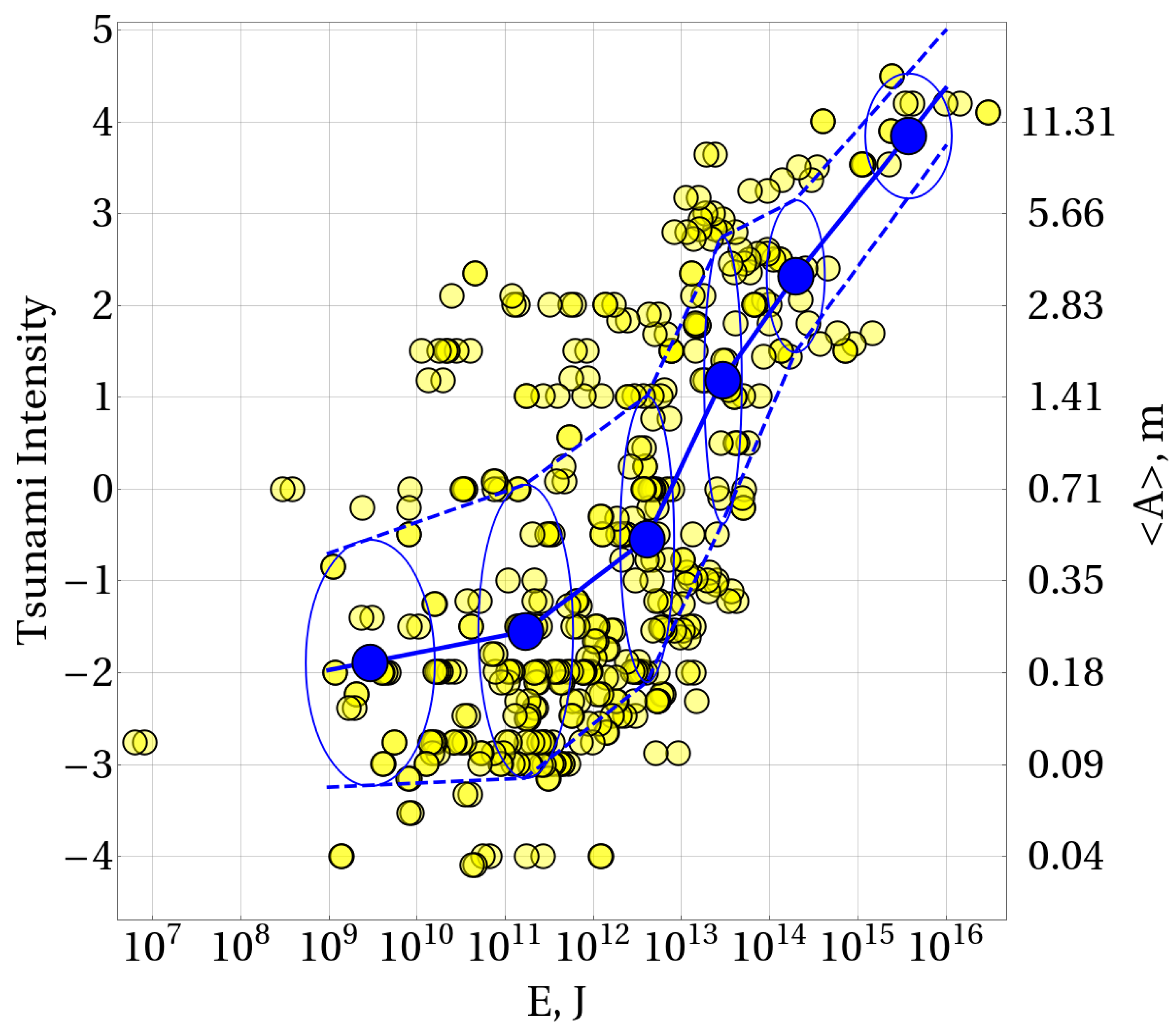
2.4. Assessment of Tsunami Intensity

The analysis of earthquake tsunami hazards was carried out on the basis of the assessment of the tsunami intensity on the Soloviev–Imamura scale, I [5,36], which was based on the value of the potential energy E of the initial elevation at the tsunami source. For this assessment, the empirical relationship between the intensity and energy obtained from historical tsunami data was used. Further, we shall describe a way to obtain this empirical relationship.

The parameters of tsunami events that were necessary for the analysis were borrowed from two publicly available historical databases that are widely known in the scientific world [1,58]: (1) the TL/ICMMG Global Historical Tsunami Database (previously known as HTDB/WLD—Historical Tsunami Database for the World Ocean; Novosibirsk, ICM & MG SB RAS) and (2) GHTD (NOAA).

Below, the two mentioned tsunami databases will be referred to as “DB1” (TL/ICMMG Global Historical Tsunami Database) and “DB2” (GHTD) for brevity. The indexes “1” and “2” will show the relation to the first or second database, respectively.

In tsunami databases, an index is assigned to each event, and this characterizes the degree of reliability of the information. In the DB1 database, this index is called the “Validity index” (5 gradations: from 0 to 4), and in the DB2 database, it is called the “Tsunami Event Validity” (6 gradations: from −1 to 4). The first criterion for selecting data on tsunami events from the DB1 and DB2 databases was a high degree of information reliability: the two upper gradations were selected (DB1: Validity index ≥ 3, DB2: Tsunami Event Validity ≥ 3).

It is known that in some cases, tsunami waves can be caused not only by earthquakes, but also by landslides (≈6%), volcanic eruptions (≈5%), and meteorological causes (≈3%), as well as by combinations of these phenomena (percentages are indicated in accordance with the DB1 database).

In the tsunami databases, a generation mechanism is specified for most events. We identified only the tsunami events for which an underwater earthquake was indicated as the source of waves—this was the second selection criterion. Combinations of sources, such as “earthquake + landslide”, “earthquake + volcanic eruption”, etc., were not considered. However, two exceptions were made to this rule: the tsunami on 1 April 1946 (Unimak Is., Aleutian Islands) and the tsunami on 28 March 1964 (Gulf of Alaska, Alaska pen.). In the databases, an earthquake and a landslide appear as the sources of these tsunamis. However, these tsunamis were characterized by rarely occurring high intensities (4.0 and 4.5, respectively) with very significant moment magnitudes of the earthquakes that caused them (8.6 and 9.1, respectively). The exclusion of these events from consideration would lead to a noticeable impoverishment of the statistics of strong tsunamis.

The third selection criterion was the moment of time starting from which there were definitions of the focal mechanism of the earthquake and seismic moment. To determine these parameters, it is necessary to have seismograms recorded by a set of stations. Recall that the beginning of the instrumental era in seismology dates back to the end of the 19th century, and seismic networks arose much later. Routine definitions of earthquake source mechanisms have been available since 1976 (Global CMT—“Global Centroid Moment Tensor database”, Columbia University and Harvard University). The first tsunamigenic earthquake for which we were able to find the definition of the mechanism of the source in scientific publications dates back to 1928 [59]. In this regard, events from 1928 onward were found in the DB1 and DB2 tsunami databases.

As the main characteristic of the strength of a tsunami, we rely on the magnitude I, which is called the intensity of the tsunami on the Soloviev–Imamura scale [5,36]. The largest number of definitions of tsunami intensity on the Soloviev–Imamura scale is contained in the DB1 database (we denote this value as I₁). The DB2 database is significantly (several times) poorer in this regard. Due to the fact that we were interested in estimating the magnitude of the tsunami intensity, the events for which the magnitude I₁ was unknown within the DB1 database were excluded from further consideration. The sample from the DB2 database could contain omissions of information on the intensity of the tsunami (I₂), but in this case, there must have been information about the maximum height of the water rise (or the runup height, H_max2). So, from the DB2 database, the events, for which the intensity, the runup height, or both were known were selected.

The DB1 and DB2 database samples formed as a result of the procedure described above contained 465 and 515 tsunami events, respectively. Further, these samples were compared with each other in order to exclude unreliable or questionable information. To achieve this goal, a cross-sample was formed, which included only the tsunami events that were present in both the DB1 and DB2 databases. Identical events were identified by minimizing the differences in times and distances between sources (tsunamigenic earthquakes) that were indicated in the DB1 and DB2 databases.

There could be no absolute coincidence of the times and positions of the sources due to the fact that information about the coordinates of an earthquake and the time of its onset was added into the DB1 and DB2 tsunami databases from various sources, and earthquakes are always localized in time and space with some error. In the cross-sample, the time difference did not exceed one minute, while the differences in the distances could be several tens of kilometers.

The cross-sample included 379 tsunami events from 1928 to 2014. Further, in accordance with the DB1 database that was involved in the cross-sample, a regression relationship was built between the intensity of a tsunami and the logarithm of the maximum runup height to base 2, measured in meters (log₂ H_max1 [m]). The pair of values I₁ and I_max1 turned out to be known for 235 events from the cross-sample. The dependence of the pairs of “intensity–runup height” values is shown in Figure 3. It can be seen that the maximum runup heights and intensity correlated very well with each other (Pearson’s correlation coefficient: 0.901). The black line in Figure 3 shows the regression curve constructed with the least squares method. The regression equation was:

I₁ = −0.206 + 0.770 log₂ H_max1 [m].

(11)

Further verification and, in some cases, correction of the data on the intensity of the tsunamis were carried out. At the same time, the specifics of the information provided in the DB2 database were taken into account—the maximum height of the water rise was, in many cases, determined by measurements from remote (sometimes thousands of kilometers from the source) sea-level stations. In this regard, the value H_max2 indicated in the DB2 database often turned out to be clearly lower than the actual level of water rise on the coast closest to the source.

Data verification and correction were implemented as follows. The intensity of a tsunami I₁ (DB1) was compared with the intensity estimated by the magnitude I_max2 (DB2). A comparison was carried out by using the regression relationship (11). In the rare cases in which there was no information about H_max2, the value I₁ was considered a reliable characteristic of the strength of the tsunami event (because there was nothing with which to compare it), and it was this value that fell into the final sample. If the information about H_max2 was present, then the final sample included the value determined by the formula

I = max[I₁, −0.206 + 0.770 log₂ H_max2].

(12)

Thus, if H_max2 was underestimated, it did not affect the initial data on the intensity of the tsunami from the DB1 database in any way. However, in cases in which the intensity I₁ was underestimated, its value was adjusted upwards—this was done in order to avoid underestimating the danger of a tsunami. We should immediately note that the correction of intensity values did not affect the data on strong tsunamis with an intensity of I > 2.

The final sample from the DB1 and DB2 tsunami databases contained information on 379 events for the period from 1928 to 2014 (dates and times of the tsunamigenic earthquakes, coordinates of the sources, definitions of the tsunami intensities I₁ and I₂, the maximum levels of water elevation H_max1 and H_max2, and adjusted intensity values I). Further, this final sample will be called TS379.

An earthquake from the Global CMT catalog was assigned to each tsunami event from the TS379 sample (Supplementary Materials). This catalog of earthquakes, in addition to the time, place, and depth of the seismic events, also contained definitions of the mechanism of the source and the seismic moment since 1976. Cross-analysis of the TS379 sample (Supplementary Materials) and the Global CMT catalog gave a list of tsunamigenic earthquakes, which contained 196 events for which the source mechanism and seismic moment are known. In addition, in scientific publications [60,61,62,63,64,65,66], information was found on the focal mechanisms for 22 other tsunamigenic earthquakes, including such well-known powerful seismic events as those on 1 April 1946 (Unimak Is., Aleutian Islands), 4 November 1952 (Kamchatka), 22 May 1960 (Chile), 28 March 1964 (Gulf of Alaska), and others. The final sample included data on 218 seismotectonic tsunami events for which information on both the intensity of the tsunami I and all data on the seismic source (Lon, Lat, h, M₀, Rake, Strike, Dip) were known; these were necessary for the calculation of the coseismic deformations of the bottom according to the Okada formulas.

Using a sample from the tsunami databases supplemented with data on the focal mechanisms of earthquakes, a retrospective analysis of the relationship between the potential energy of the initial elevations and the intensity of the tsunamis on the Soloviev–Imamura scale was carried out. Data on 218 tsunami events were analyzed. However, due to the fact that for each earthquake, there were two versions of nodal planes (two sets of Strike, Dip, and Rake angles), the calculation of the energy of the initial elevation was carried out for 436 cases.

The dependence of the tsunami Intensity upon the decimal logarithm of energy is shown in Figure 4. The dependence is characterized by a rather significant spread of data. There are no theoretical assumptions about the nature of this dependence. Therefore, to highlight the trend curve, the averaging technique was used for groups of nearby points. First, the points were sorted by energy value, and then the points were divided into groups. The numbers of points in the groups (as the energy decreased) were: 15, 30, 60, 120, 170, and 41 (in total, 436). Then, the groups of points were averaged. The average values are indicated in Figure 4 by blue dots. The blue ellipses show the values of the standard deviations (68% confidence interval). The sought dependence of intensity upon energy is shown by a broken line that passes through the blue dots. This line, as well as the dotted lines showing the 68% confidence interval, was constructed through linear interpolation of the data. In the region of the maximum and minimum energies, the dependence was slightly extrapolated to the energy values E_min = 10⁹ J and E_max = 10¹⁶ J.

Let us describe an algorithm for estimating tsunamigeneity. According to the parameters of the earthquake source, the vector field of coseismic displacements (Okada formulas) is calculated. Then, the displacement of the bottom surface is calculated, and—based on the moving average—the initial elevation in the tsunami source is determined. According to the initial elevation, the potential energy (tsunami energy) is calculated. According to the energy value, the magnitude of the tsunami intensity is determined on the Soloviev–Imamura scale by using the dependence shown in Figure 4.

If the energy value falls within the interval 10⁹ J ≤ E ≤ 10¹⁶ J, then we use the interpolation function (blue line), and we estimate the intensity of the tsunami and the 68% confidence interval. If the energy falls into the interval E < E_min = 10⁹ J, then the result of the algorithm is the conclusion that the intensity cannot be estimated (N/A). In the case in which E > E_max = 10¹⁶ J, the conclusion issued is: “high probability of a catastrophic tsunami with I > 4.5”.

The intensity of the tsunami on the Soloviev–Imamura scale is, by definition, associated with the average height of the runup on the nearest coast <A>: I = 0.5 + log₂<A>. In the graph shown in Figure 4, the left ordinate axis reflects the intensity of the tsunami, while the right one reflects the average height of the runup. Instead of intensity (or together with intensity), the algorithm can output the average height of the runup on the nearest coast.

2.5. Hydrodynamic Modeling of a Tsunami

The numerical hydrodynamic model of a tsunami used in operational calculations should give physically adequate results involving the minimal computational complexity of the task. The linear theory of long gravity waves on water meets these requirements. Indeed, in most cases, the tsunami wave length significantly exceeds the depth of the ocean. This makes it possible to apply a hydrostatic approximation, within the framework of which the initial three-dimensional equations of hydrodynamics can be integrated along a vertical coordinate, which allows us to pass to the two-dimensional equations of the theory of long waves [36,51]. In addition, with the exception of the narrow coastal strip and the runup zone, the amplitude of the tsunami is significantly less than the depth of the ocean, which makes it possible to apply linearized equations.

For hydrodynamic modeling of a tsunami in the Tsunami Observer system, linear equations of long waves written in spherical coordinates are used. The equations are solved on a uniform Arakawa C-grid type with an explicit finite difference method (e.g., [67]). The stability of the numerical scheme is provided by the choice of a time step while taking the Courant–Friedrichs–Levy condition into account.

The initial elevation of the water surface was used as the initial condition, the method of calculation of which was described in Section 2.3. The initial flow velocity field was assumed to be zero. On the isobath of 10 m, the condition of reflection (non-flow) was set, and on the outer borders passing through the ocean, the non-reflecting condition was set.

The GEBCO bathymetric dataset was used for calculations (The GEBCO_2014 Grid, version 20150318, https://www.gebco.net, (accessed on 1 May 2022). The space increment in the computational grid was set to 1 arcmin.

The center of the calculated area coincides with the projection of the center of the fault area onto the Earth’s surface. The size of the calculation domain is set depending on the moment magnitude of the earthquake. The maximum estimated time is calculated based on the size of the estimated area and the median depth of the ocean in this area.

As a result of numerical hydrodynamic modeling, an animation of the dynamics of tsunami wave propagation is formed, and the spatial distribution of the maximum displacement of the free surface is calculated, which clearly demonstrates the directions of propagation and the areas of concentration of the wave energy.

3. Results

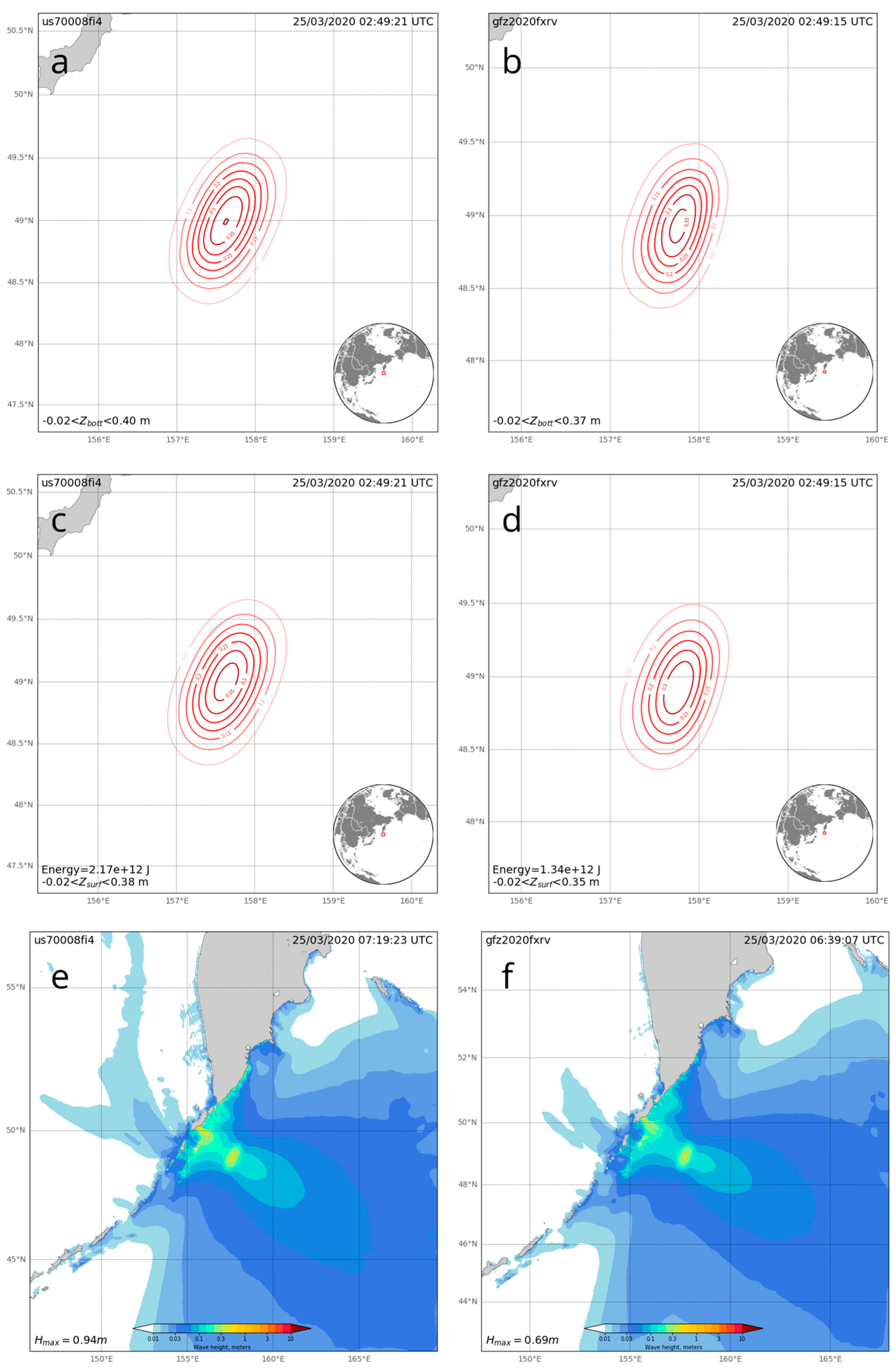
3.1. Example of the “Tsunami Observer” System’s Operation

We shall illustrate the operation of the “Tsunami Observer” system with a concrete example. On 25 March 2020, there were an earthquake and tsunami in the Northern Kurils. The magnitude of the earthquake was M_w 7.4, and the data on the focal mechanism were received in 20 min from the USGS and in 88 min from GEOFON. The results of the operation of the Tsunami Observer system for this event are available at: https://ocean.phys.msu.ru/projects/tsunami-observer/?id=us70008fi4, (accessed on 1 May 2022), https://ocean.phys.msu.ru/projects/tsunami-observer/?id=gfz2020fxrv, (accessed on 1 May 2022).

The intensity of the possible tsunami on the Soloviev–Imamura scale was estimated by the system to be 0.7 ± 1.6 (USGS) and −0.9 ± 1.6 (GEOFON), which approximately corresponds to an average tsunami height of about 0.4 m at the nearest coast.

Figure 5a,b show the coseismic bottom displacements calculated by the system from the USGS and GEOFON data, respectively. It can be seen that both versions of the focal mechanism of this earthquake were, on the whole, similar, which was confirmed by the bottom displacements having practically the same shape and amplitude, which reached 0.4 m. It can be noted that, in accordance with the GEOFON data, the origin was shifted approximately 6 km to the southeast. Figure 5c,d show the initial elevations of the water surface at the tsunami source. Taking the smoothing effect of the water layer into account (e.g., [31,34]) resulted in an insignificant (by 0.02 m) decrease in the amplitude of the water surface displacement as compared to the amplitude of the coseismic bottom displacement.

The distribution of the maximum heights of tsunami waves in the area of the northern Kurils and Kamchatka is shown in Figure 5e,f. According to the hydrodynamic modeling that was performed, the tsunami runup height in southern Paramushir Is. could be up to 1 m. According to GHTD data, the tsunami height in the city of Severo-Kurilsk (northern Paramushir Is., eyewitness observation) was 0.5 m, which corresponds quite well with the system estimates.

3.2. Results of Operation of the “Tsunami Observer” System

Since the start of its operation (from 28 January 2018 to 1 August 2022), the system has processed 560 seismic events based on USGS data and 587 based on GEOFON data. The tsunami intensity was determined for 170 and 150 of these events, respectively; these events were defined by the system to be potentially tsunamigenic. From the NIED F-net data, 14 seismic events were processed, and three of them were recognized as tsunamigenic events. This small number of events based on the data of the NIED F-net system is due to its regional status and the fact that its tracking by the “Tsunami Observer” system began only on 1 December 2020.

During the considered period of the Tsunami Observer system’s operation (from 28 January 2018 to 1 August 2022), 44 tsunami events of a seismotectonic nature occurred according to the GHTD data (Cause Code = 1, 2, 3, 4, 5; Validity ≥ Definite Tsunami). In only 5 of these 44 cases, the maximum runup exceeded 1 m.

Of the 44 above-mentioned tsunami events, the Tsunami Observer system tracked 41 and missed 3. The first of the missed events occurred on 6 May 2018 near Honshu Island (Japan). According to the sole observation, the maximum runup did not exceed 0.15 m. In this case, the earthquake magnitude was M_w 5.4, which was below the system’s response threshold. Two other missed events were processed by the system, but these earthquakes were recognized as non-tsunamigenic, i.e., the system did not estimate their intensity on the Soloviev–Imamura scale. The reaction adequacy of the system in these two cases was confirmed by the registration of waves of a centimeter amplitude (7 February 2020, Puerto Rico, M_w: 6.4, maximum runup: 0.06 m (eight observations); 18 March 2021, Algeria, M_w: 6.0, maximum runup: 0.06 m (four observations)).

Figure 6 shows a comparison of the maximum tsunami runups according to the GHTD data and the maximum tsunami wave heights according to the results of hydrodynamic the modeling performed by the Tsunami Observer system. It should be emphasized that the comparison included the maximum wave heights over the entire computational domain. As a rule, the maxima were reached near the shore. From Figure 6, it can be seen that in 75% of all of the cases, the maximum wave height estimate differed from the observed values by no more than a factor of 5; the corresponding corridors are marked with black dotted lines. Next, we will comment on the cases for which there was a significant underestimation or overestimation of runup heights (events that lay outside the specified corridor).

The points in the lower-right corner of the plot in Figure 6 correspond to the three events in which the Tsunami Observer system significantly underestimated the runup heights. Now, let us consider the cases of underestimation in more detail.

The number 1 in Figure 6 denotes the points corresponding to the tsunami on 30 October 2020 in Turkey (M_w 7.0). The consequences of this event have been investigated by several expeditions [68,69,70]. There are 272 records of recorded tsunami runups in the GHTD database. The maximum tsunami runup on the basis of which the points were plotted was 5.3 m. This runup was most probably due to the local topographical features of a subgrid scale. The average runup height for this event was 1.2 m, which matched the system estimate much better.

The number 2 in Figure 6 marks the points corresponding to the tsunami on 5 August 2018 in Indonesia (M_w 6.9). Runups with heights of 1.7 and 2 m were established by subjective evidence from eyewitnesses near the tsunami source at distances of 15 and 30 km from the source. Instrumental registration of the wave heights was made at a greater distance (more than 60 km), and the wave heights from these data did not exceed 0.1 m, which is in reasonable agreement with the system’s assessment.

The number 3 in Figure 6 indicates the point corresponding to the tsunami on 28 July 2018 in Indonesia (M_w 6.5 GEOFON, M_w 6.4 USGS). This case was similar to the previous one. In the GHTD database, there were data on two observations of tsunami wave heights from eyewitnesses (1 and 2.5 m), and there were no objective instrumental measurements. In this case, either the eyewitnesses overestimated the wave heights or the runups were due to some local effects, e.g., landslides.

The overestimated tsunami hazards (the points in the upper-left corner of the plot in Figure 6) refer to fairly strong earthquakes that occurred at a considerable distance from the locations where the tsunami waves were recorded.

The tsunami event on 29 July 2021 near Kodiak Island, Alaska is marked with number 4. The tsunami was caused by a strong earthquake with an M_w value of 8.2. Based on the focal mechanism, the system showed a maximum wave height of up to 4.5 m. The GHTD database contained data on three cases of the registration of this tsunami at source distances over 350 km, and the measured wave heights were up to 0.25 m. There were no data on tsunami manifestation in the near field.

The number 5 marks the tsunami event on 22 July 2020 on the Shumagin Islands, Alaska. The tsunami was caused by an earthquake with an M_w value of 7.8. There was a fact of coastal registration of a wave height of 0.24 m at a distance of 130 km from the epicenter. In the other eight points of registration, which were distant from the source at a distance from 400 to 1700 km, the wave heights did not exceed 0.05 m. In the near field, the wave heights could certainly be closer to the estimates given by the Tsunami Observer system (~1 m). The other cases of overestimation of the earthquake tsunami hazard referred to events with centimeter-high runup heights, and it makes no practical sense to discuss them.

A very important issue influencing the possibility of using the “Tsunami Observer” system as an auxiliary tool for early tsunami warning is the timeliness of the arrival of information on an earthquake’s origin mechanism. Figure 7 presents the time delays of information arrival concerning a source in the case of the three databases: USGS, GEOFON, and NIED. The figure is plotted for all of the data from 28 January 2018 to 1 August 2022.

The right part of Figure 7 presents histograms for each of the databases, which show the numbers of events in the delay time intervals. It may be noted that the GEOFON service prepares data on focal mechanisms somewhat more operatively in comparison with USGS. The focal mechanisms of earthquakes are determined automatically in NIED without the participation of on-duty seismologists, so the information is obtained much faster—7–8 min—after the earthquake.

The left part of Figure 7 presents the time delays as a function of the moment magnitudes of earthquakes. It can be seen that, for most seismic events, a significant magnitude is a kind of mobilizing factor: for M_w > 7, the delay rarely exceeds one hour, while for weaker events, the delays can amount to several days.

The possibility of using the Finite Fault Model (FFM) in operational tsunami forecasting is periodically discussed in the scientific literature [3,71,72]. The time delays of the relevant data (USGS) are also shown in Figure 7. It can be seen that FFM data accessibly appear at best 2 h after a seismic event, but usually several days or even weeks later. Such long delays indicate that it is actually impossible to use FFM for early tsunami warning. It should also be noted that the FFM is calculated only for sufficiently strong earthquakes (usually M_w > 7).

4. Discussion

In this paper, we purposefully did not discuss the speed of the Tsunami Observer system because it is largely determined by the computing power used. However, in the first stage, the system depends entirely on delays in the arrival of external information about the earthquake. The stage of calculation of potential tsunami energy and estimation of tsunami intensity according to the Soloviev–Imamura scale is already quite fast, taking no more than one minute on a personal computer. The hydrodynamic modeling stage has the greatest potential for speeding up the system. The numerical model used in the current version applies a structured grid with a fixed step for the latitude and longitude, which is not optimal. The most promising, here, are adaptive meshes with steps related to the distribution of ocean depths. The use of such grids will allow one to significantly (by thousands of times) speed up the calculation of tsunami wave propagation [73].

In subsequent versions of the Tsunami Observer system, it is planned to introduce the possibility of calculating the tsunami source by using the Finite Fault Model. As mentioned in the previous section, the delays in FFM data arrival are so great that this model improvement will, in the near future, be for research purposes only, but not for practical purposes.

Another step in the development of the system should be to automate the downloading of data from deep-sea-level stations, such as DART (and possibly others). Comparison of the results of numerical modeling of a tsunami and the actually measured waves will enable a rapid assessment of the adequacy of the numerical reproduction of tsunami events.

There are also some prospects for “teaching” the system by dynamically loading data about tsunami events from available databases, such as GHTD. This will make it possible to refine the empirical relationships used, which should eventually have a positive effect on the predictive capabilities of the “Tsunami Observer” system.

References

1. National Geophysical Data Center/World Data Service: NCEI/WDS Global Historical Tsunami Database; NOAA National Centers for Environmental Information: Asheville, NC, USA, 2022. [CrossRef]
2. Bernard, E.; Titov, V. Evolution of tsunami warning systems and products. Phil. Trans. R. Soc. A 2015, 373, 20140371. [Google Scholar] [CrossRef] [PubMed]
3. An, C.; Liu, H.; Ren, Z.; Yuan, Y. Prediction of tsunami waves by uniform slip models. J. Geophys. Res. Ocean 2018, 123, 8366–8382. [Google Scholar] [CrossRef]
4. Chebrov, D.V. Processing center “Petropavlovsk” in seismic subsystem of Tsunami Warning System in Russian Far East in 2010–2018. Comput. Technol. 2019, 24, 120–135. (In Russian) [Google Scholar] [CrossRef]
5. Papadopoulos, G.A.; Imamura, F.; Nosov, M.; Charalampakis, M. Tsunami magnitude scales. In Geological Records of Tsunamis and Other Extreme Waves; Engel, M., Pilarczyk, J., May, S.M., Brill, D., Garrett, E., Eds.; Elsevier: Amsterdam, The Netherlands, 2020; pp. 33–46. [Google Scholar]
6. Selva, J.; Lorito, S.; Volpe, M.; Romano, F.; Tonini, R.; Perfetti, P.; Amato, A. Probabilistic tsunami forecasting for early warning. Nat. Commun. 2021, 12, 5677. [Google Scholar] [CrossRef]
7. Okal, E.A. Tsunamigenic earthquakes: Past and present milestones. Pure Appl. Geophys. 2011, 168, 969–995. [Google Scholar] [CrossRef]
8. Gusiakov, V.K. Magnitude-geographical criterion for operational tsunami prognosis: Analysis of application in 1958–2009. Seism. Instrum. 2010, 46, 5–21. (In Russian) [Google Scholar] [CrossRef]
9. Tinti, S.; Graziani, L.; Brizuela, B.; Maramai, A.; Gallazzi, S. Applicability of the decision matrix of North Eastern Atlantic, Mediterranean and connected seas Tsunami Warning System to the Italian tsunamis. Nat. Hazards Earth Syst. Sci. 2012, 12, 843–857. [Google Scholar] [CrossRef] [Green Version]
10. Hoshiba, M.; Ozaki, T. Earthquake Early Warning and Tsunami Warning of the Japan Meteorological Agency, and Their Performance in the 2011 off the Pacific Coast of Tohoku Earthquake Mw 9.0. In Early Warning for Geological Disasters; Springer: Berlin, Germany, 2014; pp. 1–28. [Google Scholar]
11. Tang, L.; Titov, V.V.; Bernard, E.N.; Wei, Y.; Chamberlin, C.D.; Newman, J.C.; Mofjeld, H.O.; Arcas, D.; Eble, M.C.; Moore, C.; et al. Direct energy estimation of the 2011 Japan tsunami using deep-ocean pressure measurements. J. Geophys. Res. Ocean 2012, 117, C08008. [Google Scholar] [CrossRef]
12. Kanamori, H. W phase. Geophys. Res. Lett. 1993, 20, 1691–1694. [Google Scholar] [CrossRef]
13. Rivera, L.; Kanamori, H. Using W phase for regional tsunami warning and rapid earthquake hazard assessment. In Proceedings of the 2nd International Workshop on Earthquake Early Warning, Kyoto, Japan, 21–22 April 2009. [Google Scholar]
14. Riquelme, S.; Bravo, F.; Melgar, D.; Benavente, R.; Geng, J.; Barrientos, S.; Campos, J. W phase source inversion using high-rate regional GPS data for large earthquakes. Geophys. Res. Lett. 2016, 43, 3178–3185. [Google Scholar] [CrossRef] [Green Version]
15. Riquelme, S.; Medina, M.; Bravo, F.; Barrientos, S.; Campos, J.; Cisternas, A. W-phase real-time implementation and network expansion from 2012 to 2017: The experience in Chile. Seismol. Res. Lett. 2018, 89, 2237–2248. [Google Scholar] [CrossRef]
16. Hirshorn, B.; Weinstein, S.; Wang, D.; Koyanagi, K.; Becker, N.; McCreery, C. Earthquake Source Parameters: Rapid Estimates for Tsunami Forecasts and Warnings. In Complexity in Tsunamis, Volcanoes, and their Hazards; Tilling, R.I., Ed.; Springer US: New York, NY, USA, 2022; pp. 299–333. [Google Scholar] [CrossRef]
17. Yokota, Y.; Ishikawa, T.; Watanabe, S.I. Seafloor crustal deformation data along the subduction zones around Japan obtained by GNSS-A observations. Sci. Data 2018, 5, 180182. [Google Scholar] [CrossRef] [PubMed]
18. Larson, K.M.; Bodin, P.; Gomberg, J. Using 1-Hz GPS data to measure deformations caused by the Denali fault earthquake. Science 2003, 300, 1421–1424. [Google Scholar] [CrossRef] [PubMed] [Green Version]
19. Langbein, J.; Bock, Y. High-rate real-time GPS network at Parkfield: Utility for detecting fault slip and seismic displacements. Geophys. Res. Lett. 2004, 31, L15S20. [Google Scholar] [CrossRef] [Green Version]
20. Wright, T.J.; Houlié, N.; Hildyard, M.; Iwabuchi, T. Real-time, reliable magnitudes for large earthquakes from 1 Hz GPS precise point positioning: The 2011 Tohoku-Oki (Japan) earthquake. Geophys. Res. Lett. 2012, 39, L12302. [Google Scholar] [CrossRef] [Green Version]
21. Grapenthin, R.; Johanson, I.; Allen, R.M. The 2014 Mw 6.0 Napa earthquake, California: Observations from real-time GPS-enhanced earthquake early warning. Geophys. Res. Lett. 2014, 41, 8269–8276. [Google Scholar] [CrossRef]
22. Minson, S.E.; Murray, J.R.; Langbein, J.O.; Gomberg, J.S. Real-time inversions for finite fault slip models and rupture geometry based on high-rate GPS data. J. Geophys. Res. Solid Earth 2014, 119, 3201–3231. [Google Scholar] [CrossRef]
23. Crowell, B.W.; Schmidt, D.A.; Bodin, P.; Vidale, J.E.; Baker, B.; Barrientos, S.; Geng, J. G-FAST earthquake early warning potential for great earthquakes in Chile. Seismol. Res. Lett. 2018, 89, 542–556. [Google Scholar] [CrossRef]
24. Kawamoto, S.; Ohta, Y.; Hiyama, Y.; Todoriki, M.; Nishimura, T.; Furuya, T.; Sato, Y.; Yahagi, T.; Miyagawa, K. REGARD: A new GNSS-based real-time finite fault modeling system for GEONET. J. Geophys. Res. Solid Earth 2017, 122, 1324–1349. [Google Scholar] [CrossRef]
25. Käufl, P.; Valentine, A.P.; O’Toole, T.B.; Trampert, J. A framework for fast probabilistic centroid-moment-tensor determination—Inversion of regional static displacement measurements. Geophys. J. Int. 2014, 196, 1676–1693. [Google Scholar] [CrossRef] [Green Version]
26. Melgar, D.; Bock, Y.; Crowell, B.W. Real-time centroid moment tensor determination for large earthquakes from local and regional displacement records. Geophys. J. Int. 2012, 188, 703–718. [Google Scholar] [CrossRef] [Green Version]
27. O’Toole, T.B.; Valentine, A.P.; Woodhouse, J.H. Earthquake source parameters from GPS-measured static displacements with potential for real-time application. Geophys. Res. Lett. 2013, 40, 60–65. [Google Scholar] [CrossRef] [Green Version]
28. Miyazaki, S.I.; Larson, K.M.; Choi, K.; Hikima, K.; Koketsu, K.; Bodin, P.; Haase, J.; Emore, G.; Yamagiwa, A. Modeling the rupture process of the 2003 September 25 Tokachi-Oki (Hokkaido) earthquake using 1-Hz GPS data. Geophys. Res. Lett. 2004, 31, L21603. [Google Scholar] [CrossRef] [Green Version]
29. Langbein, J.; Borcherdt, R.; Dreger, D.; Fletcher, J.; Hardebeck, J.L.; Hellweg, M.; Ji, C.; Johnston, M.; Murray, J.R.; Nadeau, R.; et al. Preliminary report on the 28 September 2004, M 6.0 Parkfield, California earthquake. Seismol. Res. Lett. 2005, 76, 10–26. [Google Scholar] [CrossRef]
30. Melgar, D.; Crowell, B.W.; Bock, Y.; Haase, J.S. Rapid modeling of the 2011 Mw 9.0 Tohoku-Oki earthquake with seismogeodesy. Geophys. Res. Lett. 2013, 40, 2963–2968. [Google Scholar] [CrossRef]
31. Titov, V.V.; González, F.I.; Bernard, E.N.; Eble, M.C.; Mofjeld, H.O.; Newman, J.C.; Venturato, A.J. Real-time tsunami forecasting: Challenges and solutions. Nat. Hazards 2005, 35, 35–41. [Google Scholar] [CrossRef]
32. Bernard, E.; Titov, V. Improving tsunami forecast skill using deep ocean observations. Mar. Technol. Soc. J. 2006, 40, 86–89. [Google Scholar] [CrossRef]
33. Nosov, M.A.; Grigorieva, S.S. Tsunami forecasting based on deepwater-station data. Mosc. Univ. Phys. Bull. 2015, 70, 326–332. [Google Scholar] [CrossRef]
34. Gusman, A.R.; Sheehan, A.F.; Satake, K.; Heidarzadeh, M.; Mulia, I.E.; Maeda, T. Tsunami data assimilation of Cascadia seafloor pressure gauge records from the 2012 Haida Gwaii earthquake. Geophys. Res. Lett. 2016, 43, 4189–4196. [Google Scholar] [CrossRef] [Green Version]
35. Wang, Y.; Tsushima, H.; Satake, K.; Navarrete, P. Review on recent progress in near-field tsunami forecasting using offshore tsunami measurements: Source inversion and data assimilation. Pure Appl. Geophys. 2021, 178, 5109–5128. [Google Scholar] [CrossRef]
36. Levin, B.W.; Nosov, M.A. Physics of Tsunamis, 2nd ed.; Springer International Publishing AG: Cham, Switzerland, 2016; 388p. [Google Scholar]
37. Saito, T. Tsunami Generation and Propagation; Springer: Tokyo, Japan, 2019; 265p. [Google Scholar]
38. Sementsov, K.A.; Nosov, M.A.; Kolesov, S.V.; Karpov, V.A.; Matsumoto, H.; Kaneda, Y. Free gravity waves in the ocean excited by seismic surface waves: Observations and numerical simulations. J. Geophys. Res. Ocean 2019, 124, 8468–8484. [Google Scholar] [CrossRef]
39. Lotto, G.C.; Nava, G.; Dunham, E.M. Should tsunami simulations include a nonzero initial horizontal velocity? Earth Planets Space 2017, 69, 1–14. [Google Scholar] [CrossRef] [Green Version]
40. Saito, T. Tsunami generation: Validity and limitations of conventional theories. Geophys. J. Int. 2017, 210, 1888–1900. [Google Scholar] [CrossRef]
41. Ji, C.; Wald, D.J.; Helmberger, D.V. Source description of the 1999 Hector Mine, California, earthquake, part I: Wavelet domain inversion theory and resolution analysis. Bull. Seismol. Soc. Am. 2002, 92, 1192–1207. [Google Scholar] [CrossRef] [Green Version]
42. Ammon, C.J.; Ji, C.; Thio, H.K.; Robinson, D.; Ni, S.; Hjorleifsdottir, V.; Wald, D. Rupture process of the 2004 Sumatra-Andaman earthquake. Science 2005, 308, 1133–1139. [Google Scholar] [CrossRef] [PubMed] [Green Version]
43. Shao, G.; Li, X.; Ji, C.; Maeda, T. Focal mechanism and slip history of the 2011 Mw 9.1 off the Pacific coast of Tohoku Earthquake, constrained with teleseismic body and surface waves. Earth Planets Space 2011, 63, 559–564. [Google Scholar] [CrossRef] [Green Version]
44. Tomita, F.; Iinuma, T.; Ohta, Y.; Hino, R.; Kido, M.; Uchida, N. Improvement on spatial resolution of a coseismic slip distribution using postseismic geodetic data through a viscoelastic inversion. Earth Planets Space 2020, 72, 1–24. [Google Scholar] [CrossRef]
45. Okada, Y. Surface deformation due to shear and tensile faults in a half-space. Bull. Seismol. Soc. Am. 1985, 75, 1135–1154. [Google Scholar] [CrossRef]
46. Leonard, M. Earthquake fault scaling: Self-consistent relating of rupture length, width, average displacement, and moment release. Bull. Seismol. Soc. Am. 2010, 100, 1971–1988. [Google Scholar] [CrossRef]
47. Kanamori, H.; Brodsky, E.E. The physics of earthquakes. Rep. Prog. Phys. 2004, 67, 1429. [Google Scholar] [CrossRef]
48. Tanioka, Y.; Satake, K. Tsunami generation by horizontal displacement of ocean bottom. Geophys. Res. Lett. 1996, 23, 861–864. [Google Scholar] [CrossRef] [Green Version]
49. Nosov, M.A.; Bolshakova, A.V.; Kolesov, S.V. Displaced water volume, potential energy of initial elevation, and tsunami intensity: Analysis of recent tsunami events. Pure Appl. Geophys. 2014, 171, 3515–3525. [Google Scholar] [CrossRef]
50. Bolshakova, A.V.; Nosov, M.A.; Kolesov, S.V. The properties of co-seismic deformations of the ocean bottom as indicated by the slip-distribution data in tsunamigenic earthquake sources. Mosc. Univ. Phys. Bull. 2015, 70, 62–67. [Google Scholar] [CrossRef]
51. Saito, T.; Kubota, T. Tsunami modelling for the deep sea and inside focal areas. Annu. Rev. Earth Planet. Sci. 2020, 48, 121–145. [Google Scholar] [CrossRef]
52. Kajiura, K. The leading wave of a tsunami. Bull. Earthq. Res. Inst. Univ. Tokyo 1963, 41, 535–571. [Google Scholar]
53. Tanioka, Y.; Seno, T. Sediment effect on tsunami generation of the 1896 Sanriku tsunami earthquake. Geophys. Res. Lett. 2001, 28, 3389–3392. [Google Scholar] [CrossRef] [Green Version]
54. Saito, T.; Furumura, T. Three-dimensional tsunami generation simulation due to sea-bottom deformation and its interpretation based on the linear theory. Geophys. J. Int. 2009, 178, 877–888. [Google Scholar] [CrossRef]
55. Nosov, M.A.; Kolesov, S.V. Optimal initial conditions for simulation of seismotectonic tsunamis. Pure Appl. Geophys. 2011, 168, 1223–1237. [Google Scholar] [CrossRef]
56. Nosov, M.A.; Sementsov, K.A. Calculation of the initial elevation at the tsunami source using analytical solutions. Izv. Atmos. Ocean. Phys. 2014, 50, 539–546. [Google Scholar] [CrossRef]
57. Okal, E.A.; Synolakis, C.E. A theoretical comparison of tsunamis from dislocations and landslides. Pure Appl. Geophys. 2003, 160, 2177–2188. [Google Scholar] [CrossRef]
58. Gusiakov, V.K. Tsunami history: Recorded. Sea 2009, 15, 23–53. [Google Scholar]
59. Okal, E.A. Use of the mantle magnitude M m for the reassessment of the moment of historical earthquakes. Pure Appl. Geophys. 1992, 139, 17–57. [Google Scholar] [CrossRef]
60. Kikuchi, M.; Fukao, Y. Inversion of long-period P-waves from great earthquakes along subduction zones. Tectonophysics 1987, 144, 231–247. [Google Scholar] [CrossRef]
61. Ma, K.F.; Kanamori, H.; Satake, K. Mechanism of the 1975 Kalapana, Hawaii, earthquake inferred from tsunami data. J. Geophys. Res. Solid Earth 1999, 104, 13153–13167. [Google Scholar] [CrossRef]
62. Okal, E.A. Seismic parameters controlling far-field tsunami amplitudes: A review. Nat. Hazards 1988, 1, 67–96. [Google Scholar] [CrossRef]
63. Tichelaar, B.W.; Ruff, L.J. Depth of seismic coupling along subduction zones. J. Geophys. Res. Solid Earth 1993, 98, 2017–2037. [Google Scholar] [CrossRef]
64. Johnson, J.M.; Satake, K. Estimation of seismic moment and slip distribution of the 1 April 1946, Aleutian tsunami earthquake. J. Geophys. Res. Solid Earth 1997, 102, 11765–11774. [Google Scholar] [CrossRef]
65. Johnson, J.M.; Satake, K. Asperity Distribution of the 1952 Great Kamchatka Earthquake and its Relation to Future Earthquake Potential in Kamchatka. In Seismogenic and Tsunamigenic Processes in Shallow Subduction Zones. Pageoph Topical Volumes; Sauber, J., Dmowska, R., Eds.; Birkhäuser: Basel, Switzerland, 1999; pp. 541–553. [Google Scholar] [CrossRef]
66. Barrientos, S.E.; Ward, S.N. The 1960 Chile earthquake: Inversion for slip distribution from surface deformation. Geophys. J. Int. 1990, 103, 589–598. [Google Scholar] [CrossRef] [Green Version]
67. Kämpf, J. Ocean Modelling for Beginners: Using Open-Source Software; Springer: Berlin/Heidelberg, Germany, 2009. [Google Scholar]
68. Dogan, G.G.; Yalciner, A.C.; Yuksel, Y.; Ulutaş, E.; Polat, J.; Güler, I.; Şahin, C.; Tarih, A.; Kânoğlu, U. The 30 October 2020 Aegean Sea Tsunami: Post-Event Field Survey Along Turkish Coast. Pure Appl. Geophys. 2021, 178, 785–812. [Google Scholar] [CrossRef]
69. Kalligeris, N.; Skanavis, V.; Charalampakis, M.; Melis, N.S.; Voukouvalas, E.; Annunziato, A.; Synolakis, C.E. Field survey of the 30 October 2020 Samos (Aegean Sea) tsunami in the Greek islands. Bull. Earthq. Eng 2021, 1–33. [Google Scholar] [CrossRef]
70. Aksoy, M.E. Post-event field observations in the İzmir-Sığacık village for the tsunami of the 30 October 2020 Samos (Greece) Mw 6.9 earthquake. Acta Geophys. 2021, 69, 1113–1125. [Google Scholar] [CrossRef]
71. Riquelme, S.; Fuentes, M.; Hayes, G.P.; Campos, J. A rapid estimation of near-field tsunami runup. J. Geophys. Res. Solid Earth 2015, 120, 6487–6500. [Google Scholar] [CrossRef]
72. Melgar, D.; Williamson, A.L.; Salazar-Monroy, E.F. Differences between heterogenous and homogenous slip in regional tsunami hazards modelling. Geophys. J. Int. 2019, 219, 553–562. [Google Scholar] [CrossRef]
73. Nosov, M.A. Adapting a mesh when simulating tsunami waves. Math. Models Comput. Simul. 2018, 10, 431–440. [Google Scholar] [CrossRef]
Figure 1. Architecture of the “Tsunami Observer” system.
Geosciences 12 00455 g001
Figure 2. Geometry of the source model.
Geosciences 12 00455 g002
Figure 3. The relationship between the intensity of a tsunami on the Soloviev–Imamura scale and the maximum height of the water rise (maximum runup) in accordance with the DB1 data (235 events—circles). The black line is a regression dependence constructed with the least squares method. Pearson’s correlation coefficient is ≈0.901.
Geosciences 12 00455 g003
Figure 4. Dependence of the tsunami intensity on the Soloviev–Imamura scale on the energy of the initial elevation according to data on 218 historical events (yellow circles). The blue dots were obtained as a result of averaging the original data by group. Ellipses represent the 68% confidence interval (standard deviation). The solid line is a linear interpolation of the intensity’s dependence on energy, and the dotted lines are a linear interpolation of the 68% confidence interval.
Geosciences 12 00455 g004
Figure 5. Results of processing by the system of the tsunamigenic earthquake on 25 March 2020 in the Northern Kurils. Subfigures show the coseismic bottom displacements (a,b), the initial elevations of the water surface at the tsunami source (c,d) and distribution of the maximum heights of tsunami waves (e,f). Earthquake data origin: USGS (left column) and GEOFON (right column).
Geosciences 12 00455 g005
Figure 6. Comparison of the maximum tsunami runups from the GHTD data and the maximum tsunami amplitudes from the hydrodynamic simulations.
Geosciences 12 00455 g006
Figure 7. Time delays of information concerning earthquake sources.
Geosciences 12 00455 g007
Publisher’s Note: MDPI stays neutral with regard to jurisdictional claims in published maps and institutional affiliations.