1. Introduction
Sea level measurements are of critical importance in the verification of tsunami generation. When a large earthquake occurs in a subduction zone and the Regional Tsunami Service Providers of UNESCO/IOC issue alerts, sea level measurements are used to verify tsunami generation and take further action (i.e., the evacuation of coastal areas). However, in some cases, if the tsunami source is very close to the coast, there is not enough time between the identification of an event and the issue of alerting bulletins. In addition, when the tsunami is not generated by a large earthquake but rather by an atypical source (i.e., landslide or volcanic eruption) or prior information from the earthquake is not available before the arrival of the tsunami, it is of vital importance to have other means for the verification of tsunami generation.
The Inexpensive Device for Sea Level Measurement (IDSL) [
1,
2,
3,
4], developed at the EC-JRC, is a low-cost focused innovative sea level measurement device consisting of a Linux-based Raspberry Pi board; it is capable of acquiring, processing and moving data back into the EC-JRC data server. It runs software that allows for the measurement of sea level and its interpretation according to an algorithm to provide the detection of anomalous waves in real time.
The JRC IDSL algorithm, in the current setup of the device, provides the following three functionalities:
To create a trigger to send an email and SMS to a list of users (i.e., Tsunami Service operators).
To activate the webcam (if available) and take images every 2 min.
To start a 10 s video recording from the webcam (if available).
In principle, the triggering mechanism could also be used for other activations, such as TCP/IP receiving devices, local display boards, social media information or any other web application. However, a balance between fast activation and the avoidance of false alerts should be considered; for example, these types of alerts should only be sent to people when more than one device shows an alert. This mode was tested in the EC-funded Last Mile Projects (i.e., Kos in Greece and Marsaxlokk in Malta).
The algorithm, which is capable of acquiring, processing and moving data back into the EC-JRC data server or any other relevant database can also be used for any sea level measurement of interest with similar triggering criteria.
This study describes a model, shows a number of test cases and provides a discussion on the results. A GitHub site is also provided where all the routines can be downloaded in Python format to allow the model to be replicated on other platforms or instruments.
Tsunami Detection Models
The identification of a tsunami must be performed through the analysis of measured sea levels on the fly. The model cannot be too sophisticated as it has to be implemented in the low-cost instrument hardware itself, which generally does not have a large computation capability, although it is enough to perform most of the required operations.
A tsunami is characterized by a significant deviation from the expected tide at that moment in time, especially in regard to temporal characteristics. Therefore, in principle, with a good understanding of the background tide in the installation location, one could activate an alert related to tsunami observation when an anomaly is present. However, the tide cannot be known with great accuracy at every location, especially in places with new installations where historical data is not available. In addition, the algorithm should also have the capability to differentiate an anomaly in sea level recordings due to a tsunami from an anomaly related to meteorological effects, such as storm surges, to avoid false alerts. Anomalies can also originate from harbour activity (large ships passing nearby and creating waves) or, in the case of a radar-type sensor, small boats located below the sensor itself. In addition, extreme severe events leading to storm surges can cause waves that exceed the measuring range of the sensor. All these could create an anomaly in the signal. A detection algorithm should, as much as possible, be able to identify only tsunami-related events; various models are available in the literature to address this complexity [
5,
6,
7,
8,
9].
One of the first implementations of such an algorithm in real time was performed by NOAA in DART buoys [
6] to determine the low frequency tide by using an interpolation of the last 3 h. This threshold was used to perform a higher frequency data acquisition (one point every 15 s instead of one point every 1 h to save transmission time through satellite).
Many authors have studied methods to analyse these events in real time, for example, F. Chierici et al. [
7] proposed a method based on the estimation of the tide for a specific location using a tidal effect removal based on a harmonics analysis of the least square method. Bressan et al. [
8] used a method called TEDA that was based on the instantaneous slope of the signal and the difference between two windows of different lengths to define an alerting function. Y. Wang et al. [
9] proposed a method that adaptively decomposed the time series into a set of intrinsic mode functions, where the tsunami signals of ocean-bottom pressure gauges (OBPGs) were automatically separated from the tidal signals, seismic signals and background noise. In a follow-up paper [
10], Y. Wang and K. Satake demonstrated their tsunami detection algorithm that used ensemble empirical mode decomposition to extract the tsunami signals, retrospectively imitating real-time operations for tsunami early warning.
To our knowledge, excluding DART, none of these methods have been routinely applied in real or near real-time tsunami monitoring. On the other hand, the first JRC model was installed in tide gauges in July 2013 and has been in operation since then.
2. Materials and Methods
The current study used tide gauge records from available online databases, including GLOSS (
https://www.ioc-sealevelmonitoring.org, accessed on 5 September 2022) [
11] and the European Commission Sea Level Database TAD-Server (
https://webcritech.jrc.ec.europa.eu/TAD_server, accessed on 5 September 2022), which offers online real-time sea level measurements. Other data tools such as the ones listed in [
12] may allow for easy data downloads by researchers and students. As described in
Appendix A, we also developed a new application that may be useful in identifying interesting tsunami data, named Sea Level Machine
Those data were used in order to prepare and optimize an innovative algorithm that was then implemented in the software contained inside instruments, such as the IDSL (Inexpensive Device for Sea Level Measurements), to allow for proper real-time analysis.
This article sets the requirements of this algorithm and mentions other already available methods that can be used to detect the presence of an abnormal wave. It proposes a method to optimize and verify the constants present in the algorithm and finally shows what the results of its application during real-time events.
The JRC Tsunami Verification Algorithm
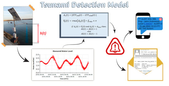
The primary goal of tsunami detection in the continuous flow of sea level data, with one data sample every few seconds in the best case, is to differentiate and identify the signal (tsunami) from the noise (all sea level changes that are not due to a tsunami). This is achieved through the estimation at each new data acquisition of the absolute difference between the long-term forecast (LTF) and the short-term forecast (STF), one of the most broadly used algorithms in weak-motion seismology [
5]. The LTF is an estimation of the value of the current point, performed by calculating the least square second-order polynomial related to a long period (1.5–3 h of data), whereas the STF is the same quantity estimated using a shorter time window (10–20 min). Therefore, the difference tends to identify changes in sea level due to tsunamis with a specific period range without being confused by individual outliers (i.e., a sudden individual value in the normal values). However, for very noisy signals, the change could be due to an increase in noise. Therefore, in order to identify a point as an alert, we compare the absolute difference between LTF and STF with the root mean square (RMS) of the signal: when the difference exceeds a number of times, the RMS the alert level increases by 1 unit, and when it comes back below the threshold, the alert level decreases by 1 unit. The maximum value of the alert level is 10.
The algorithm is based on the following equation:
where
is the alert signal, computed as the absolute value of the difference between the STF and LTF computed at a given time of (
t). The STF and LTF represent the expected value at the current time t, obtained via the second-order least square method estimated using two different times, typically 15 min and 2 h. However, these periods are strictly related to the installation site for which testing is necessary before assigning the final values of the integration times.
The variation component is calculated by computing the root mean square of the alert signal over the long-term period, multiplying by a constant and adding a constant to be sure that a small change in sea level does not cause an alert for very smooth signals. According to our experience, the values of the multiplication factor and the constant can be set at 4 and 0.1 m, respectively, to start; however, the final constants must be chosen by analysing the results of the measurements. In particular, if a signal is too noisy, an increase in integration time is necessary, keeping in mind that too large an integration time for the LTF can cause a delay in the computed curve and should be avoided.
The logic of the alerts is computed by comparing
and
:
The alert level (AL) is increased by 1 unit at each acquisition time interval with a maximum value of 10. In Equation (3) Amin represents a minimum amplitude that should be exceeded to give an alert.
The difference between our STF/LTF method and the STA/LTA method used in seismology for triggering high frequency data acquisition is that in the STA/LTA process, the ratio between the average amplitudes is adopted; in our case, with STF/LTF, we use the difference between the estimated value at the current time using the previous points. This is necessary because in the case of seismic signals, the long-term signals essentially oscillate around a baseline value, while in the case of sea level, the influence of the tide may be relevant in certain cases; therefore, it is not possible to average the signals in the long term.
3. Results
3.1. Data Examples
An example from a device that was recently installed in Rakata Island, Indonesia, for the period between 24 May 2022 18:00 and 25 May 2022 06:00 during a tide cycle is demonstrated in
Figure 1.
When we zoom into the 1 h period,
Figure 2, the various curves are more clearly observed; the short-term signal follows the trend of the signal but eliminates the high frequency peaks that are normally present in such signals due to small waves and reflections in the ports. In the case of measurements performed slightly offshore without port protection, as in this case, the formation of waves is always possible.
By taking the difference between the short and long term and comparing it with the value of the RMS (multiplied by a factor), we can judge if the alert is reached,
Figure 3. Another condition for alerting is that the estimated amplitude is larger than a predefined value (i.e., 5 cm).
The reason for using both the RMS and the threshold in (1) is that when a signal is very noisy, it is important that the signal overpasses the normal oscillations to avoid the generation of an alert for each oscillation. On the other hand, a threshold is still necessary in order to avoid that the other extreme, where a very smooth signal with very small oscillations, even in the range of 1 mm, generates an alert. In short, both the RMS with its multiplier and the threshold value should be considered. The values we found to be reasonable as starting values are 4 as the RMS multiplier and 0.1 m as the threshold; however, this parameter should be calibrated after the operation of the instrument for some time.
A similar mechanism to those described above has been implemented by JRC in the tide gauges installed in Greece by the SIAP company (Koroni, Paleochora and Kythira) and in the IDSL measurements. At the moment, more than 35 devices have this algorithm implemented on board; when an alert condition is identified, an email and SMS are sent to a distribution list (
Figure 4). In addition, the computing algorithm has also been implemented in the Italian tide gauges installed by ISPRA.
3.2. Optimization of Parameters
The process of determining the natural frequency of the ports where the instrument is located is a key first step for every new installation or sea level signal for which the procedure is applied. Two examples of this application are presented below.
3.2.1. Saidia Marina, Morocco
The level is shown in
Figure 5; the signal power spectrum analysis (
Figure 6) revealed that this marina is characterized by a small period between 26 and 35 min oscillations above the normal astronomical tide.
Considering that the time interval between the points was 6 s, it was necessary to average the small period oscillations a number of times, i.e., 4–5 times, which resulted in a time of 80–110 minutes, or, in terms of the number of points, 800–1100 points.
The effect of the number of points on the quality of the long-term average (orange curve) can be seen in
Figure 7.
An increase in the N300 parameter (number of intervals of acquisition, 5 s) tended to better represent the average for an oscillating signal like the one recorded in Saidia Marina (Morocco). If the value of N300 is too low, the LTF will follow the curve too closely. The final value of the parameter was therefore chosen as 1200 points in order to follow the real average of the curve.
3.2.2. Le Castella, Italy
Le Castella, Italy, is a much smaller port than Saidia Marina and the signal (
Figure 8) is characterized by a power spectrum with four typical oscillations of periods 8, 12, 18 and 22 minutes with smaller amplitudes than in the case of Saidia Marina (
Figure 9). Using a similar approach as in the case of Saidia Marina and considering 12 min as the characteristic period, we limited the long-term average period to 48–60 min and therefore the number of points, with a 6 s interval, to 480–600 points maximum.
For Le Castella, looking at the response by varying the number of points, it appears that 600 points (1 h average) was sufficient; there was no need to go to 1200 points, which tends to delay the average (
Figure 10).
3.3. Software Implementation Options
The JRC detection algorithm has been directly implemented in the individual hard-drives of instruments (Raspberry Pi) using various languages (c, C# and Python3); however, remote computation possibilities also exist for instruments that do not have on-site computational capabilities or that are closed systems where it is not possible to install local software. The installation of local computation makes the instrument independent from the network and the availability of other computers; in addition, it is also possible to connect local networks and issue alerts in the absence of a large connecting network. On the other hand, remote computation has the advantage that the instrument software can be simple, and the computation backlog can be passed off to powerful machines in a computing centre. In some cases, both options (
Figure 11) have been being exploited for testing purposes and to ensure redundancy.
3.4. Performance of the JRC Tsunami Verification Algorithm during Real Events
The following three cases are presented below to demonstrate the performance of the algorithm:
Algeria earthquake, 18 March 2021 00:04, M 6.0—alert was not activated
Krakatoa tsunami, 22 December 2018—alert could have been activated
Hunga Tonga volcanic eruption—alert was activated
3.4.1. Algeria Earthquake, 18 March 2021 00:04, M 6.0
This was a relatively small tsunami event, caused by the M6 earthquake that occurred in Algeria; the tsunami was recorded by a number of stations in the Mediterranean Sea. One of these was Marina di Teulada, in the south of Sardinia, Italy. The event caused an anomaly of about 8.5 cm above the normal tide at around 01:10 UTC (
Figure 12). As the alerting limit (given by RMS*4 + 0.1) was 14 cm, the alert level was not activated. Soon after this event, due to the increased oscillation, the RMS limit increased and therefore an alert activation became more unlikely unless a much larger oscillation could take place. It is important to identify the first alert event so analysts can carefully look into this and many other signals.
3.4.2. Krakatoa Tsunami, 22 December 2018
On 22 December 2018, a large tsunami was generated by a flank collapse of the Krakatau volcano inside the Anak Krakatau volcanic complex. The tsunami hit the coasts of Sumatra and Java in the Sunda Strait with waves up to 6–8 m, causing more than 400 fatalities along the coasts of Sunda Strait. The tsunami arrived at the location whose signal is presented in the following figure at about 21:30 local time (14:30 UTC) on 22 December, completely unexpected, and caused fatalities and extensive damage along the coastal areas of the Sunda Strait.
At the time of the event, there was no specific tsunami detection instrument installed around the volcano. The first instrument reached by the wave was the Marina Jambu tide gauge belonging to Badan Informasi Geospasial (BIG) of Indonesia with a 1 min sampling rate. In
Figure 13, the recorded sea level is shown. If the detection algorithm had been applied to the recorded data, an alert would have been triggered.
3.4.3. Hunga Tonga Volcanic Eruption, Prigi, Indonesia Signal
The explosion of the Hunga-Tonga volcano on 15th January 2022 04:15 UTC resulted in a tsunami that devastated the areas surrounding the volcano. In addition, the pressure wave from the explosion generated a sea level disturbance that was observed all over the world and detected by several tide gauges. In many tide gauge signals, this oscillation was sufficient to trigger an alert.
About 7 h after the explosion, the pressure wave reached IDSL-308, located in Prigi, south of Java, resulting in a sea level anomaly with a variation up to 30 cm above the tide level, as shown in
Figure 14. The detection algorithm identified the event, resulting in the activation of the webcam at 13:14 UTC (20:14 local time,
Figure 15) and the release of email and SMS alerts to registered users, as shown in
Figure 16.
4. Discussion
In this study, a simple algorithm developed and installed by the JRC was presented, and some examples of this algorithm’s capacity to verify the occurrence of a tsunami were provided. The algorithm has been used in the IDSL devices since 2014; since then, a number of events have been identified. It was shown that the model is able to identify important events in addition to small events, if the quality of the sea level signal is sufficiently smooth such that the RMS of the signal stays low; if this is the case, tsunamis only tens of centimetres tall can be identified. If a signal is noisy, then only tsunamis with significant wave heights can be detected.
The quality of the recorded sea level data plays a significant role in the successful performance of this algorithm: in the case where a spurious peak is present in the data, if not properly excluded from the acquired data (for example by excluding points with a variation from one point to another of more than a reasonable amount), these variations are reflected in the short-term forecast and therefore also in the alerting value. This can consequently result in a false alert. To avoid such a situation, it would be ideal to have another instrument installed close by to ensure that the alert is triggered only based on both observations. Such a deployment could also prevent the activation of alerts as the result of possible disturbances due to the position—below or close to the acoustic cone below the sensor—of an object, person, boat etc.
The correct parameters of the model should be chosen after an analysis of the first data from a period of at least 1–2 weeks. A reliable method to pre-calculate the values of the optimal parameters in advance has yet to be found.
This processing could be performed for each of the tide gauges around the world before acquiring data from any database, such as the JRC Sea Level Database or the GLOSS Sea Level Facility. This would allow for the activation of alerts the combination of two or three tide gauges and send an overall basin alert. This processing will require sufficient computing power to perform all the estimations for all the sea level measurements acquired.
5. Conclusions
The simple algorithm presented here has been implemented since 2014 in more than 40 devices that monitor sea level and estimate in real time the potential tsunami threat. In some cases, spurious activations have occurred with the presence of a boat below the sensor. For this reason, if used in operational systems, a double verification with two devices in the same area—but not too close each other—is strongly recommended.
Using this model for a number of real cases, its ability to detect and alert to the presence of anomalous waves in few minutes was demonstrated. In one case (Hunga Tonga volcano eruption), it automatically triggered SMS and email alerts.
The correct parameters for the model should be chosen after an analysis of the data from a period of at least 1–2 weeks. This was performed for the IDSL devices and with these parameters, they are able to correctly identify ongoing events
This same algorithm is also being used for other sea level data from around the world obtained from a number of public sites (IOC-GLOSS, DART, NOAA, INCOIS, etc.); however, the calibration of constants for more than 2500 devices is not optimal. A reliable method to pre-calculate the optimal parameter values has yet to be found and would be extremely useful.


