1. Introduction
Snow is a key component of the Earth’s climate system through its effect on the surface energy balance and its critical role as a freshwater reservoir. Snow plays an important role as a thermal insulator that reduces heat exchange between the ground and the atmosphere and also protects plants from the very low winter temperatures. Information on snow extent, depth, snow water equivalent variation in time and space, and on melting and runoff events are all quantitative pieces of information that are needed for successful seasonal snow monitoring.
Sentinel-1 and Sentinel-2 are part of the existing satellite constellations providing very useful information for snow monitoring with the advantages of high spatial resolution and good revisit time (5–6 days over Western Europe). The Sentinel-2 mission has two identical satellites (Sentinel-2A and Sentinel-2B, launched in June 2015 and March 2017, respectively). Each one is carrying an imager that observes the Earth with 13 spectral bands at spatial resolutions that vary from 10 m (for the visible and near-infrared bands), 20 m (for the red edge) and 60 m (for shortwave infrared). The orbits of Sentinel-2 have been chosen to optimize their overall global coverage but with differences in revisit times.
While Sentinel-2 is a mission with optical instruments, the Sentinel-1 mission is a constellation of satellites carrying active microwave instruments (Synthetic Aperture Radar (SAR) at C-band) allowing observations in all weather and sunlight conditions. The Sentinel-1 mission is composed of two identical satellites (launched respectively in April 2014 and April 2016) that observe the Earth with a revisit time that varies according to the region (6 days over Western Europe) and a high spatial resolution (20 m for the Interferometric Wide (IW) swath mode). Retrieving useful information on snow from optical data is not straightforward and requires many limitations to be taken into account [
1,
2,
3]. In particular, proper handling of clouds and geometric effects of the terrain for optical measurements is necessary (snow/cloud signal separation, observations that are challenging to use in case of clouds, gap-filling rules, management of shadow effects in the mountains). For SAR data, the detection of wet snow is based on the assumption that C-band backscatters are reduced compared to snow-free or dry snow situations. Many studies have used a threshold method applied to ratio backscatter images to detect wet snow (with the use of a snow-free image as a reference, which can also be taken under dry snow or frozen ground conditions). These studies have investigated how sensitive wet snow detection is to choices of reference images and thresholds and allowed to monitor phases of snowpack moistening over areas of interest ([
4,
5,
6,
7,
8,
9,
10,
11] among many others).
The European Environment Agency, on behalf of the European Commission, funded the development and near real-time production of Copernicus High Resolution Snow and Ice (HR-S&I) to meet user needs for total snow, dry snow and wet snow estimates using measurements from Sentinel-1 and Sentinel-2. These new products have already been evaluated in various ways, notably through comparisons with in-situ measurements [
12]. However, the spatial and temporal variability of snow cover in the mountains requires further evaluation of snow products, specifically taking into account the particular characteristics of mountain areas such as altitude and orientation. Few studies have focused on representing, merging or assessing satellite-based snow products with respect to the elevation or the slope or the orientation constraints of a catchment or a massif. For instance, the study of [
13] has shown that satellite data are good at identifying the relationship between snow depth and elevation at a catchment scale. In the study of [
14], the authors used an elevation-based threshold of the SAR backscatter to better combine wet snow and total snow satellite estimates. The study of [
10] suggested a representation of total snow cover from Sentinel-2 or wet snow from Sentinel-1 that best represents the variability of snow at the scale of a mountain range taking into account elevation, slope and orientation. One should also know that the evaluation of satellite-derived wet snow cover against in situ data is less straightforward than the snow cover map because of the scarcity of snow water equivalent measurements and the non-trivial correlation between air temperature and snowpack conditions. There is also the need to establish objective scores for the evaluation of satellite products in complex terrain where in-situ measurements are rather scarce. An additional motivation of this work was to design a tool for intercomparison of satellite products that would be independent of the spatial resolution of the products and that would take into account the elevation and orientations of a massif of interest to infer the main characteristics of the wet or total snow cover.
In this article, our main focus is on the Copernicus SAR Wet Snow (SWS) product generated from Sentinel-1 measurements in mountainous terrain. For this evaluation, we also used the Copernicus Fractional Snow Cover (FSC) product when it was usable (with no/few clouds). We first introduced and used a new score named PSSP (Probabilistic Score for Satellite Products) particularly adapted for the evaluation of satellite products in mountains. Then, we computed and studied snowmelt lines from SWS products at the scale of French Alpine massifs over several seasons. We also compared the SWS product with snow simulations from the Crocus snow model. Data and models used in this study are described in
Section 2. Results are provided in
Section 3, while
Section 4 provides discussion and conclusion statements.
2. Data and Models
2.1. Study Area and Time Period
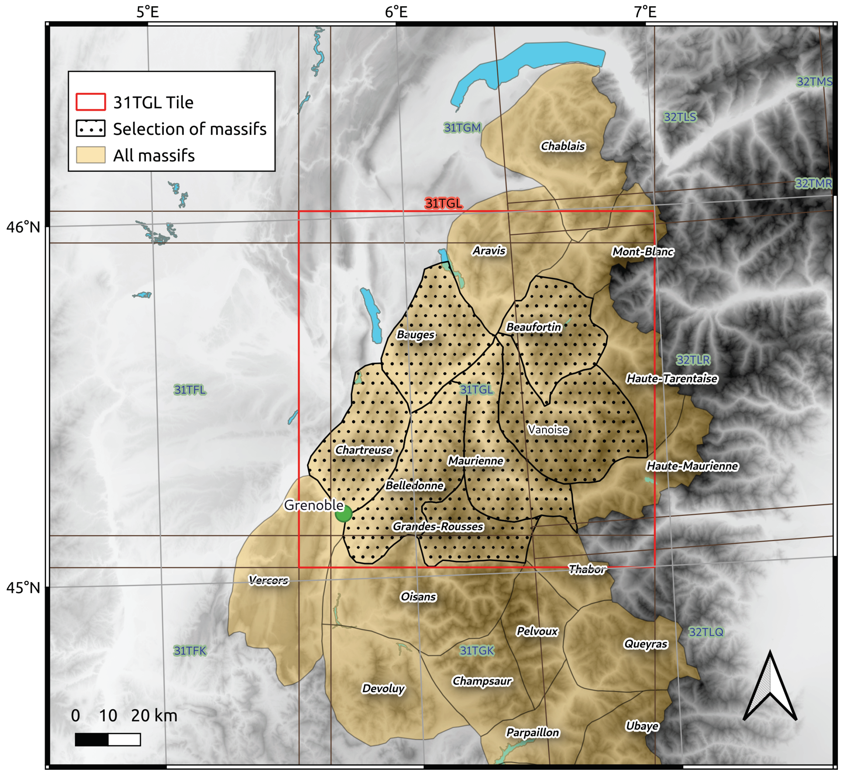
We focus on the 31TGL tile, related to Sentinel-2 tiling system/Military Grid Reference System (MGRS), located in the Northern side of the French Alps, which includes the following massifs: Grandes-Rousses, Belledonne, Chartreuse, Bauges, Beaufortain, Vanoise and Maurienne (see
Figure 1 for the test zone and location of massifs). The Grandes-Rousses massif is generally oriented north-south, with some peaks reaching 3464 m. The highest peak of the Belledonne massif, the Grand pic de Belledonne, reaches 2977 m, almost the same altitude as the highest point of the Beaufortain massif, which is the Roignais, 2995 m. The study area includes high mountain massifs with a diversity of slope orientations, vegetation cover and the presence of several high altitude lakes and glaciers. The area hosts several national parks and ski resort facilities offering significant and very diversified tourist attractions. We conducted all of our analyses at the scale of the massif to better highlight general characteristics of snow cover according to altitude and orientation. All of the investigations discussed in this article were carried out for the six massifs included in the 31TGL tile. For reasons of simplicity, we have largely relied on the results obtained for the Grandes Rousses massif, this massif being perfectly representative of a high mountain region. The study period is from the fall of 2016 to the summer of 2021.
2.2. The SAR Wet Snow (SWS) and the Fractional Snow Cover (FSC) Products
The SWS binary products are based on Sentinel-1 and are only calculated for the high mountain areas according to selected MGRS tiles covering mountain regions in the Alps, Pyrenees, Scandinavia, Iceland and East Turkey. These are selected areas from a certain altitude without any significant agricultural activity. The SWS product informs on the presence of wet snow with a spatial resolution of 60 m. Different areas are screened out in the SWS product, such as radar geometric distortion areas (shadow/layover/foreshortening), forests, urban areas, water surfaces. The algorithm used to map the extent of the snowmelt zone uses a change detection method based on the ratio of the backscatter coefficient of a surface under wet snow conditions to that under snow-free or dry snow-covered surfaces, dry snow being transparent to the C-band [
5]. We used SWS products derived from Sentinel-1 ascending orbit (relative orbit 161) and descending orbit (relative orbit 139).
The Fractional Snow Cover (FSC) product is derived from Sentinel-2 optical satellite data following the methodology described in [
12,
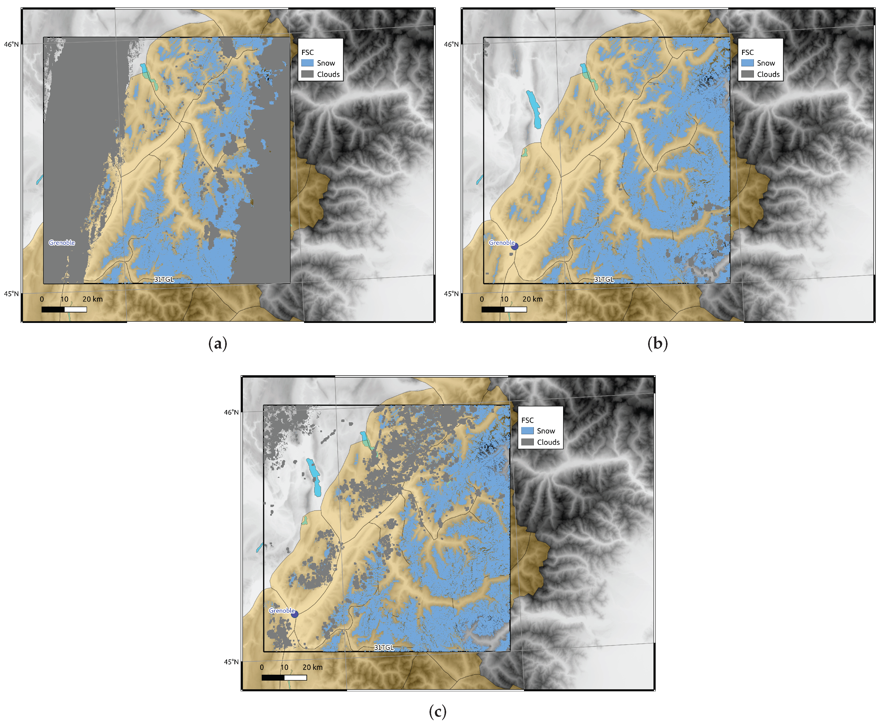
15]. The FSC product has a resolution of 20 m and provides the fraction of the surface covered by snow as well as the delimitation of areas covered by clouds for which there is no estimate of snow cover. From the snow cover fraction value, we derive the binary information: snow presence if the fraction > 0%, no snow otherwise. A detailed description of the products is provided on the Copernicus Land Monitoring Service web site
https://land.copernicus.eu/user-corner/technical-library/hrsi-snow-pum, accessed on 1 January 2022.
As stated earlier, the study period is from the fall of 2016 to the summer of 2021. We selected FSC products that fall within this period and have an acceptable cloud cover rate. The image search for an acceptable rate is done at the scale of each studied massif, not at the scale of the 31TGL tile, which allowed us to keep a large number of Sentinel-2 images, including those with a cloud rate greater than 50%. The
Figure 2,
Figure 3 and
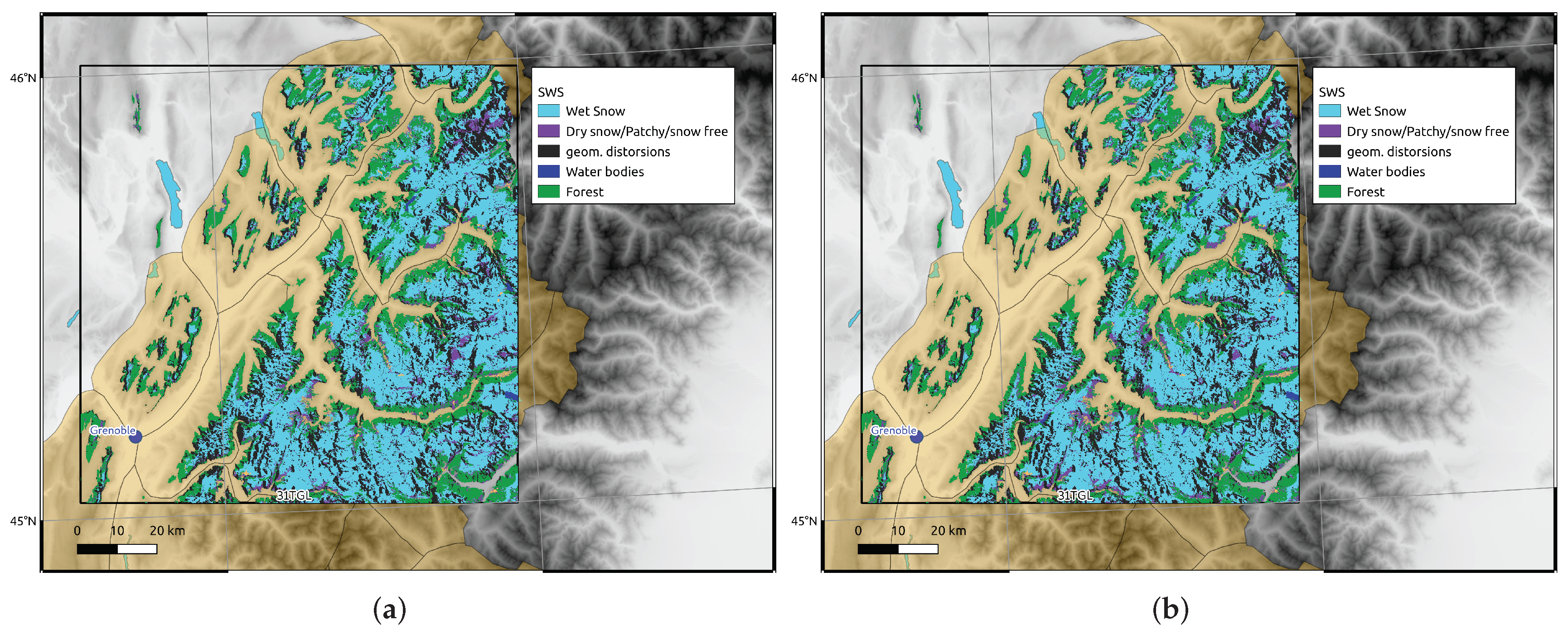
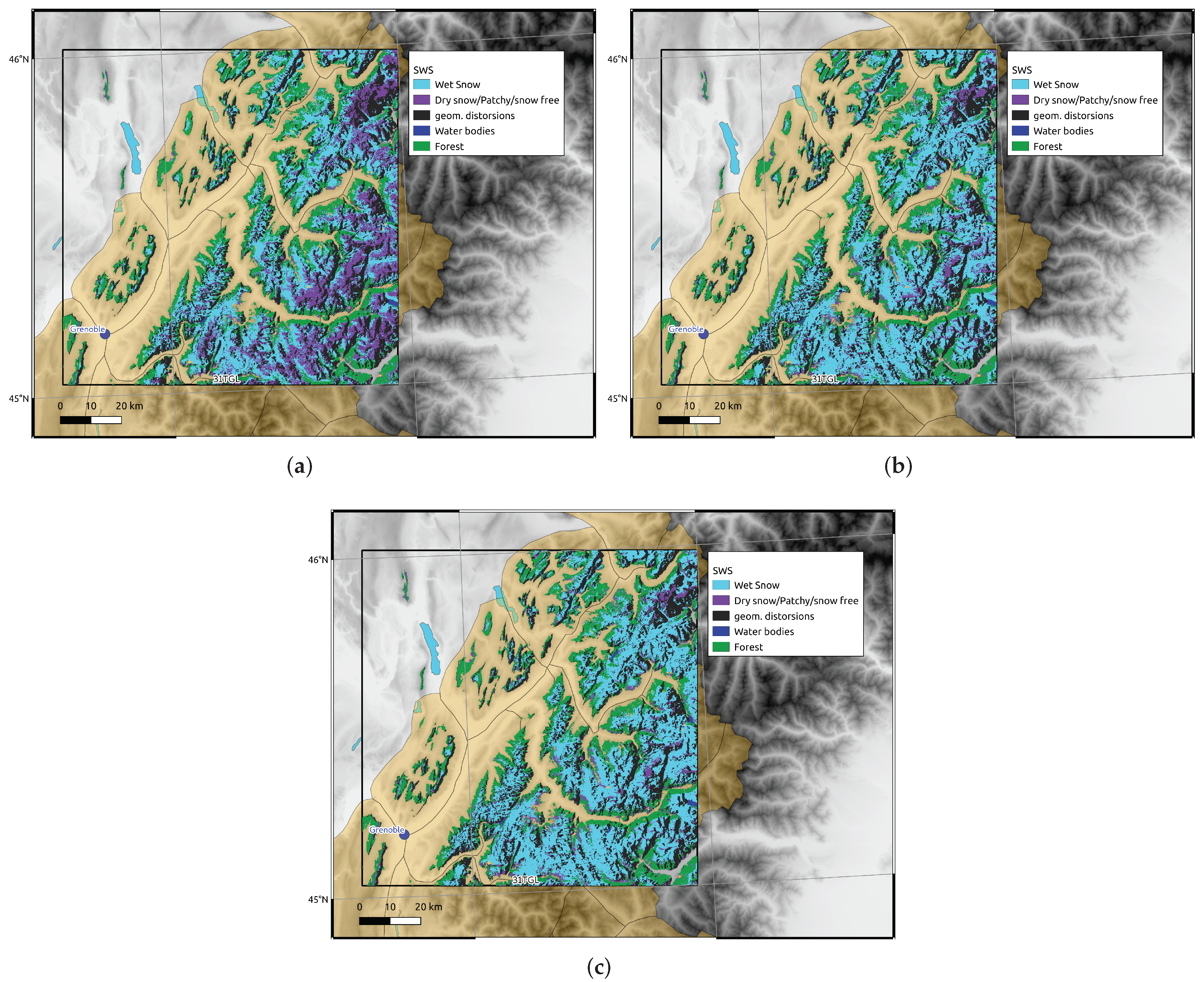
Figure 4 illustrate examples of the FSC and SWS products over a few dates in the winter of 2018 marked by an abundant overall wet snow. Cloud cover on the selected dates 15 April 2018, 20 April 2018 and 25 April 2018) is minimal, which allows access to FSC optical products. The SAR-based SWS products that are the closest to the Sentinel-2 acquisition dates have been selected: 16 April 2018 and 22 April 2018 for the ascending orbit and 15 April 2018, 21 April 2018 and 27 April 2018 for the descending orbit. For these dates, marked by an overall moistening of the snowpack, we note a very good agreement between the optical snow products. The comparison of products with maps is only qualitative and does not allow for a more in-depth comparison of the temporal variability of the different products and their dependence on the terrain characteristics. In what follows, we will consider other methods that enable us to evaluate products in more detail, taking into account the seasonality of the snow and some terrain properties (orientation, altitude).
2.3. Crocus Reanalysis
Crocus is a state-of-the-art unidimensional numerical snowpack model that allows us to simulate the physical properties of the snowpack and its evolution in time [
16,
17]. Crocus performs the thermodynamic coupling between snow and soil, as it is one of the snowpack models that can be activated with the land surface model ISBA-DIF (Interaction between Soil, Biosphere and Atmosphere, [
18,
19]). Crocus simulates different mass and energy exchange processes with the atmosphere and with the underlying ground (e.g., radiative fluxes, latent and sensible heat fluxes, precipitation) and provides a realistic vertical stratification of the snowpack (up to 50 layers). The first layer is, by convention, the atmosphere/snow layer. Each simulated snow layer is described by different properties such snow depth, albedo, temperature, grain size, snow liquid water content among other parameters. The Crocus model can be forced by observations, forecasts, analyses or reanalyses or fed by outputs from atmospheric models. In this study, we use the Crocus snow reanalyses performed at the scale of the French massifs [
20]. As the French mountains are divided into relatively homogeneous areas (23 massifs for the Alps, 23 massifs for the Pyrenees and 2 massifs for Corsica), the Crocus reanalyses can be used for this specific study in the Alps. It has been run with simulations of surface atmospheric conditions obtained from the SAFRAN model [
21]. For each of the massifs studied, we have estimates of the snowpack parameters per day by altitude, orientation and for different classes of slopes (low, medium and high slopes). We focused on the snow depth and the liquid content of the snowpack because of the high sensitivity of C-band SAR measurements to snow wetness. The liquid water content (LWC) is relative to the amount of liquid water per unit mass or volume of snow. LWC can be expressed in terms of ratios of units of mass or units of volume. The snow simulations of Crocus cover the period from August 2016 to the end of July 2021.
3. Results
3.1. A Probabilistic Score to Evaluate Satellite Products in Mountains
In order to compare the snow cover as observed by Sentinel-2 and that of Sentinel-1, we developed a new score called PSSP (a Probabilistic Score for Satellite Products) particularly adapted for mountain regions where altitudes, slopes and orientations are important elements of the terrain to take into account for a successful comparison between the different products. It is worth noting that the snow observed by Sentinel-2 is a total snow including dry and wet snow, while the snow observed by Sentinel-1 is only wet (C-band SAR mixes dry snow with snow-free zones). We will therefore use this score during periods of snowpack moistening (targeting April-May-June periods). We will first compare, at selected dates, the optical products with the products based on SAR images. The selected dates correspond to acquisitions without too many clouds. For the sake of simplicity, we target the Grandes-Rousses massif for this analysis, but the methodology is also applicable to other massifs. For each selected Sentinel-2 date, we seek for the closest Sentinel-1 dates in both ascending and descending orbits. Once all the products are selected, we compute the snow occurrence probability curves by altitude step. Since some areas are screened out in the Sentinel-1-based products (such as layover areas and forests), we proceeded to remove these areas from the Sentinel-2-based products as well (designed as S2S figure legends). We also calculated for each Sentinel-2 image the cloud rate at the scale of a massif or for some altitude ranges within a massif.
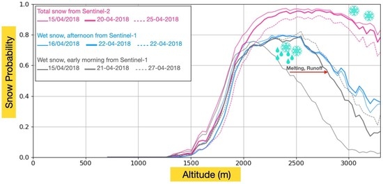
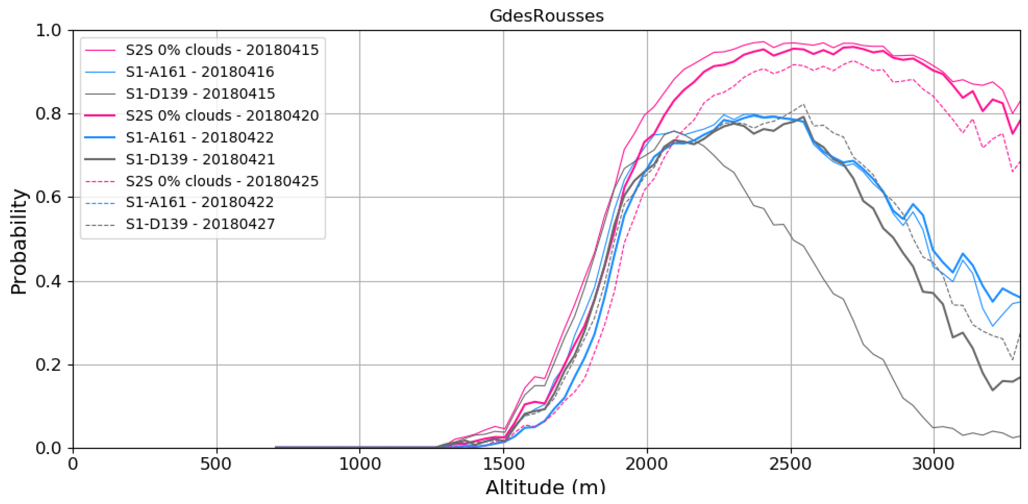
Figure 5 shows the snow occurrence probability curves obtained for three successive Sentinel-2 dates (pink curves): 15 April 2018, 20 April 2018 and 25 April 2018, for which no clouds were recorded over the Grandes-Rousses massif. The figure also shows the obtained snow probability curves from SWS products for Sentinel-1 ascending scenes observed on 16 April 2018 and 22 April 2018 (blue curves) and for Sentinel-1 descending scenes observed on 15 April 2018, 21 April 2018 and 27 April 2018 (Grey curves). Note that the snow maps for these dates are shown in
Figure 2,
Figure 3 and
Figure 4, respectively. From the probability curves, a number of insights into the snowpack condition can be deduced. For mid-April, the results show a probability of more than 80% of snow above 2000 m. Late afternoon (ascending orbit), wet snow is present at more than 75% in the 2000–2500 m altitude range and drops to less than 40% for the higher altitudes. Early in the morning (descending orbit), wet snow remains present up to 70% around 2000 m, but its probability decreases rapidly with altitude.
The curves from optical products (pink curves) are very similar, which can lead one to believe that the snowpack condition did not change from mid-April to late April 2018. The SWS product curves, on the other hand, show that the snow has changed significantly in terms of moistening. This is particularly noticeable from the descending orbit curves, which show an increase in snow probability above 2000 m on 21 April 2018 compared to the snow condition on 15 April. The increase in the extent of wet snow in the descending orbit may indicate the runoff phase [
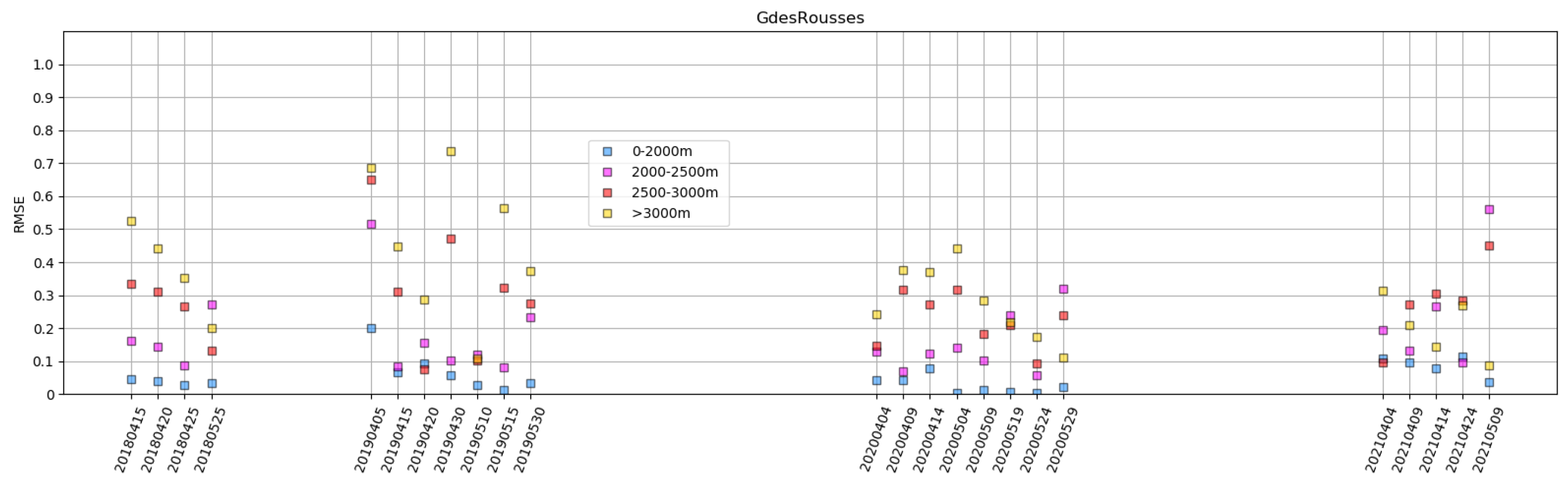
9]. We note, moreover, slightly lower probability values from Sentinel-2 for 25 April. The probability curves are very informative about the snow as seen by the satellites and can be used to evaluate the complementarity of the different products. We also calculated quantitative scores from these curves. We therefore evaluated the degree of similarity between the different probability curves. For this purpose, the computation was performed according to different altitude ranges: 0–2000, 2000–2500, 2500–3000, >3000. The different altitude ranges were chosen to match the massif used. For the Grandes-Rousses massif, nearly 70% of the pixels have an altitude <2000 m, 20% have an altitude between 2000 and 2500, 9% have an altitude between 2500 and 3000 m and only 1% with an altitude above 3000 m. These altitude ranges should therefore be adjusted according to the massif studied. For each altitude range, we calculate the Root Mean Square (RMS) errors of the differences of the probability curves (Sentinel-1 minus Sentinel-2). The result of these calculations is presented in
Figure 6 and
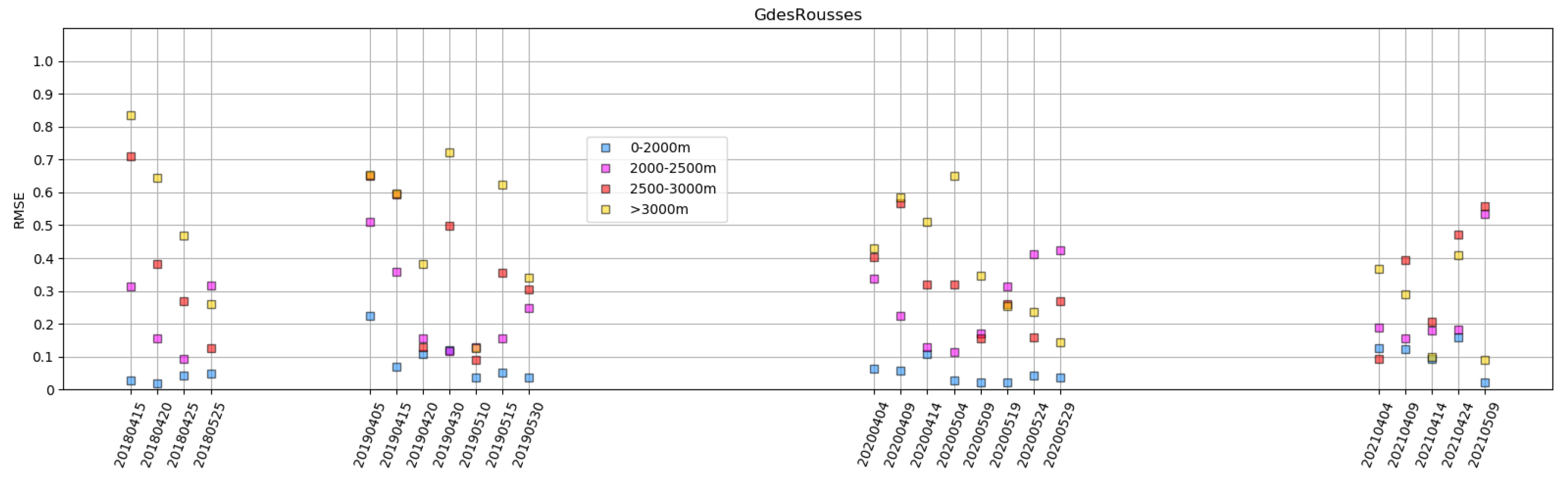
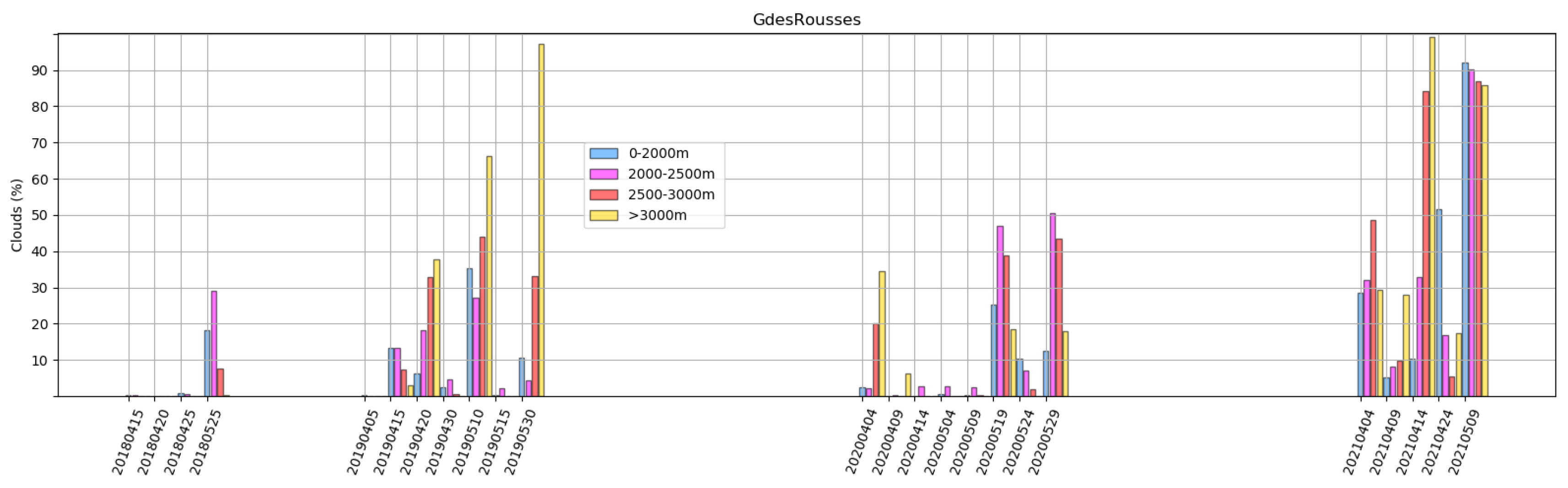
Figure 7. The figure shows the RMS errors for different dates of Sentinel-2 observations (April–May). At these dates, SWS products closest in time to S2 are selected (in ascending (panel (a)) and descending orbit (panel (b))). The results are shown by altitude range (blue squares: 0–2000 m, pink squares: 2000–2500 m, orange squares: 2500–3000 m and yellow squares: >3000 m). For each Sentinel-2 date, the cloud cover rate is also presented per altitude range (see
Figure 8). The error rms are very low for the range 0–2000 m globally less than 0.2 except for some dates where the cloud cover is high and may explain a disagreement between satellites. RMS errors are higher for high altitudes. Note that this is a set of pixels representing less than 10% for the Grandes-Rousses massif. In addition, the disagreements between satellites may be explained by the presence of dry snow, which is not detected by Sentinel-1. For the period of 2018, which is a textbook case because it is almost free of clouds, we observe a decrease of the RMS errors as the snowpack humidification is increasing for the altitude ranges above 2000 m. Other scores were also calculated such as correlations but will not be detailed here.
3.2. Meltlines from SWS Products
We also evaluated SWS products using the meltline diagnostics introduced by [
10]. In this study, the authors used a massif scale to derive Altitude-Orientation diagrams of SAR-based wet snow for different slope classes and also Altitude-Time diagrams of wet snow for different orientation classes. They have shown that this type of diagram is very useful to get an overview of the snow distribution as it makes it very easy to identify the wet snow lines for different orientations. For an orientation of interest, Altitude-Time diagrams can be used to track the evolution of the snow to locate the elevations and dates of snow loss.
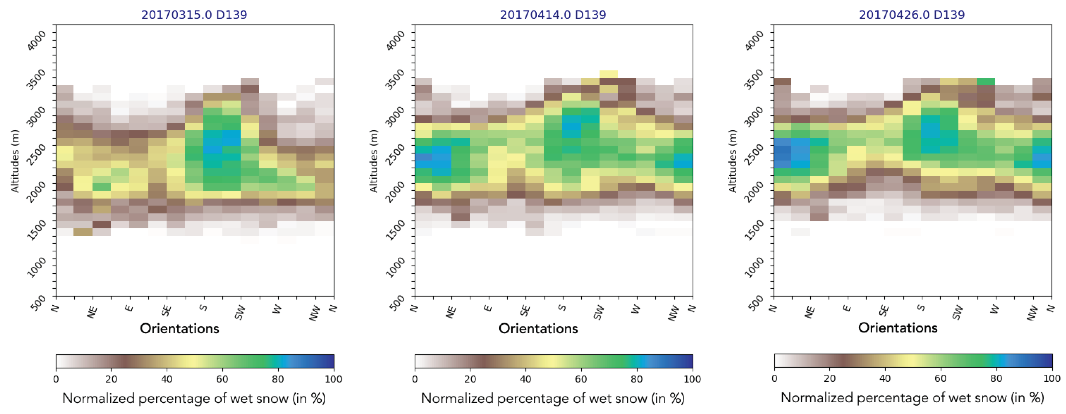
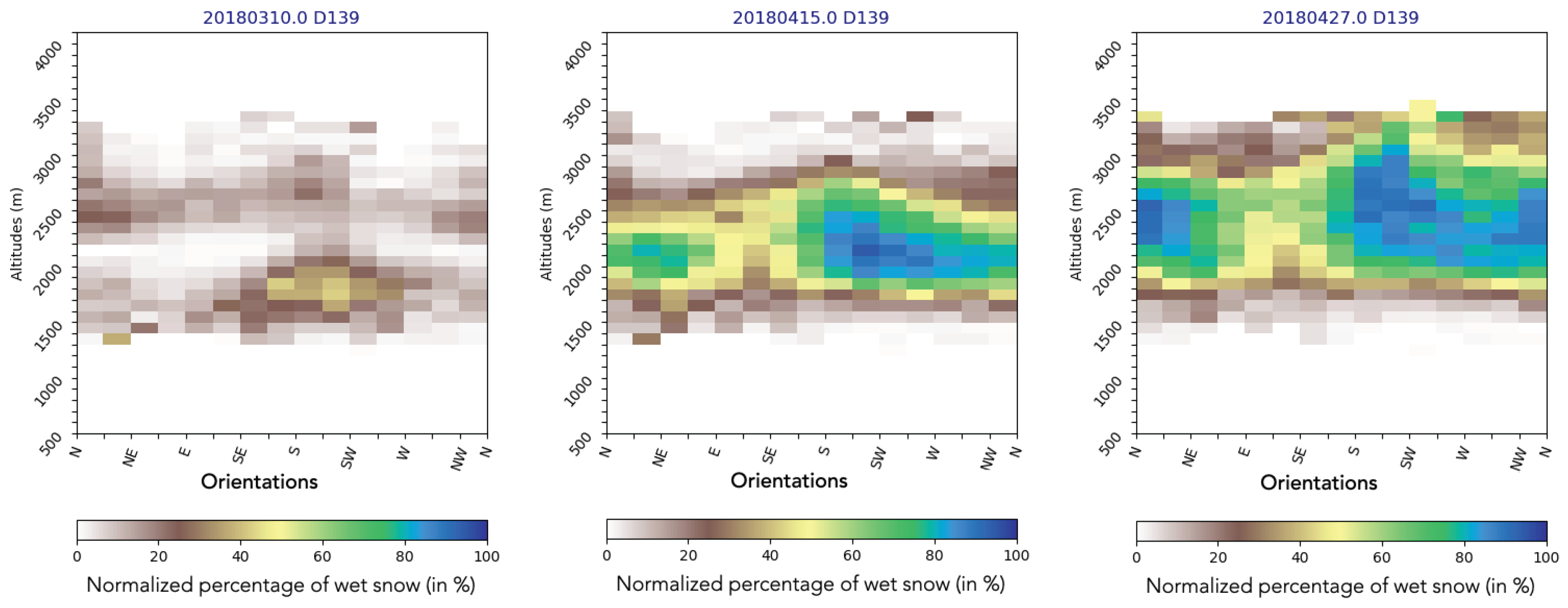
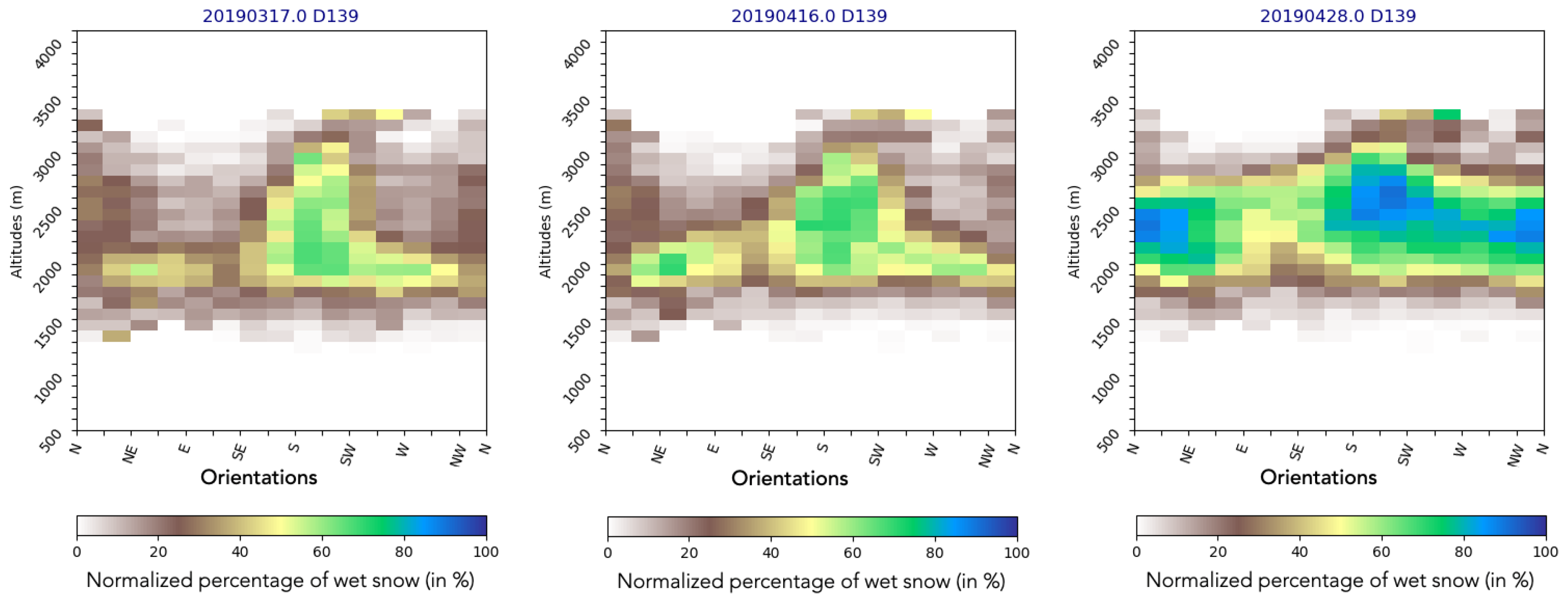
Figure 9 is an Altitude–Orientation diagram for the Grandes-Rousses massif, which shows the normalized percentage of wet snow-covered pixels by classes of elevation and orientation for the descending Sentinel-1 orbit and for mid-march, mid april and end of April 2017. The results are shown in %: 100% means that, for a given class of orientation and elevation, the snowpack can be assumed to be completely wet. If the percentage is lower, it means that a portion of the pixels is snow-free or is associated with dry snow.
Figure 10,
Figure 11,
Figure 12 and
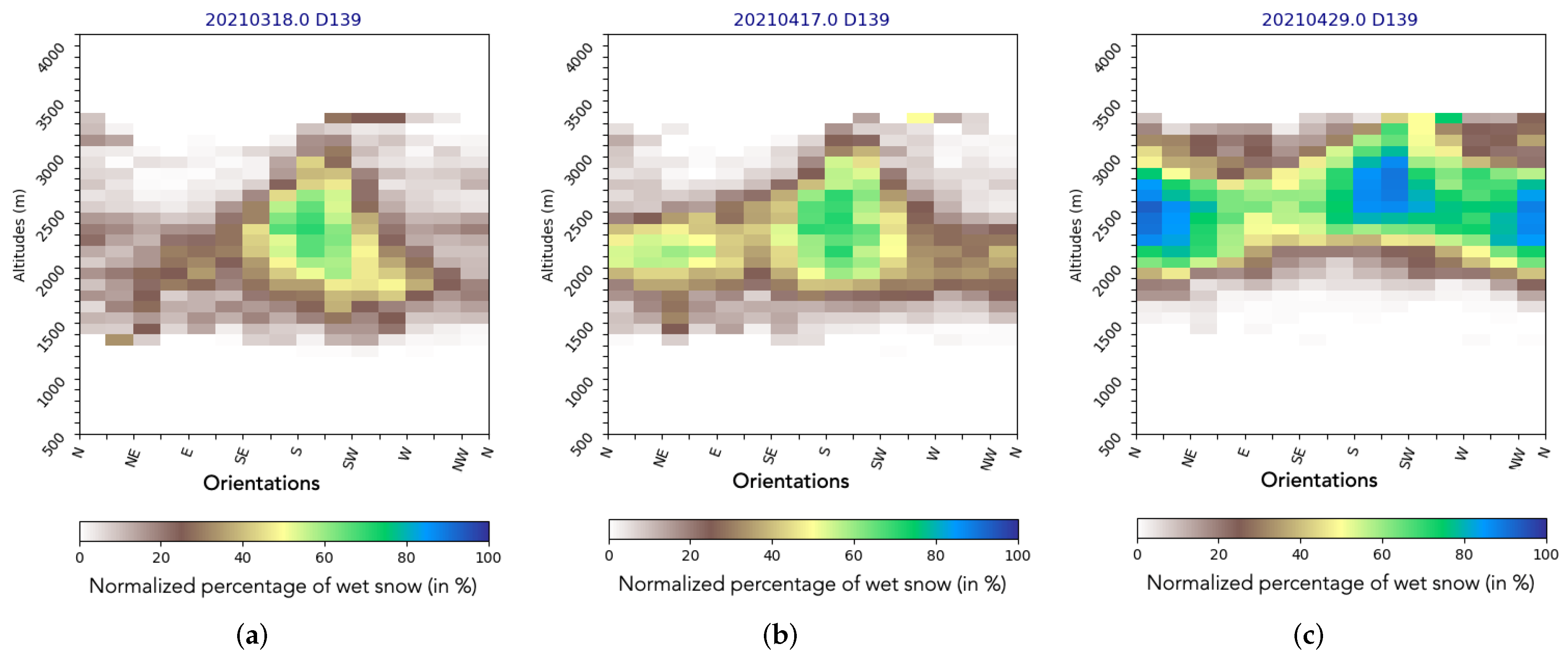
Figure 13 are similar to
Figure 9 but for springs 2018, 2019, 2020 and 2021, respectively. These diagrams give a seasonal comparison of the level of wet snow cover. In early spring, we can see that the wet snow is fairly variable from season to season.
In 2017, wet snow was present from mid-March onwards, mainly in the south-facing slopes and at altitudes up to 3000 m. In mid-April, the snow became wetter in other orientations, including the northern ones. The minimum melt line was around 2000 m (more than 50% of wet snow: yellow colors) and rises towards 2500 m by the end of April. The maximum limit of wet snow is also variable, depending on the orientation and the date. Note that we can assume that, at these altitudes, the snow is rather dry. In 2018, snow moistening occurred later than in 2017, but also more markedly with a greater presence of wet snow even at high altitudes. For 2019, wet snow remained contained in southern orientations until mid-April before expanding to other orientations. For 2020, the snow cover moistening occurred quite early and was very marked starting in mid-April. 2021 seems similar to 2019 with a wet snow cover remaining contained in the southern orientations until the end of April.
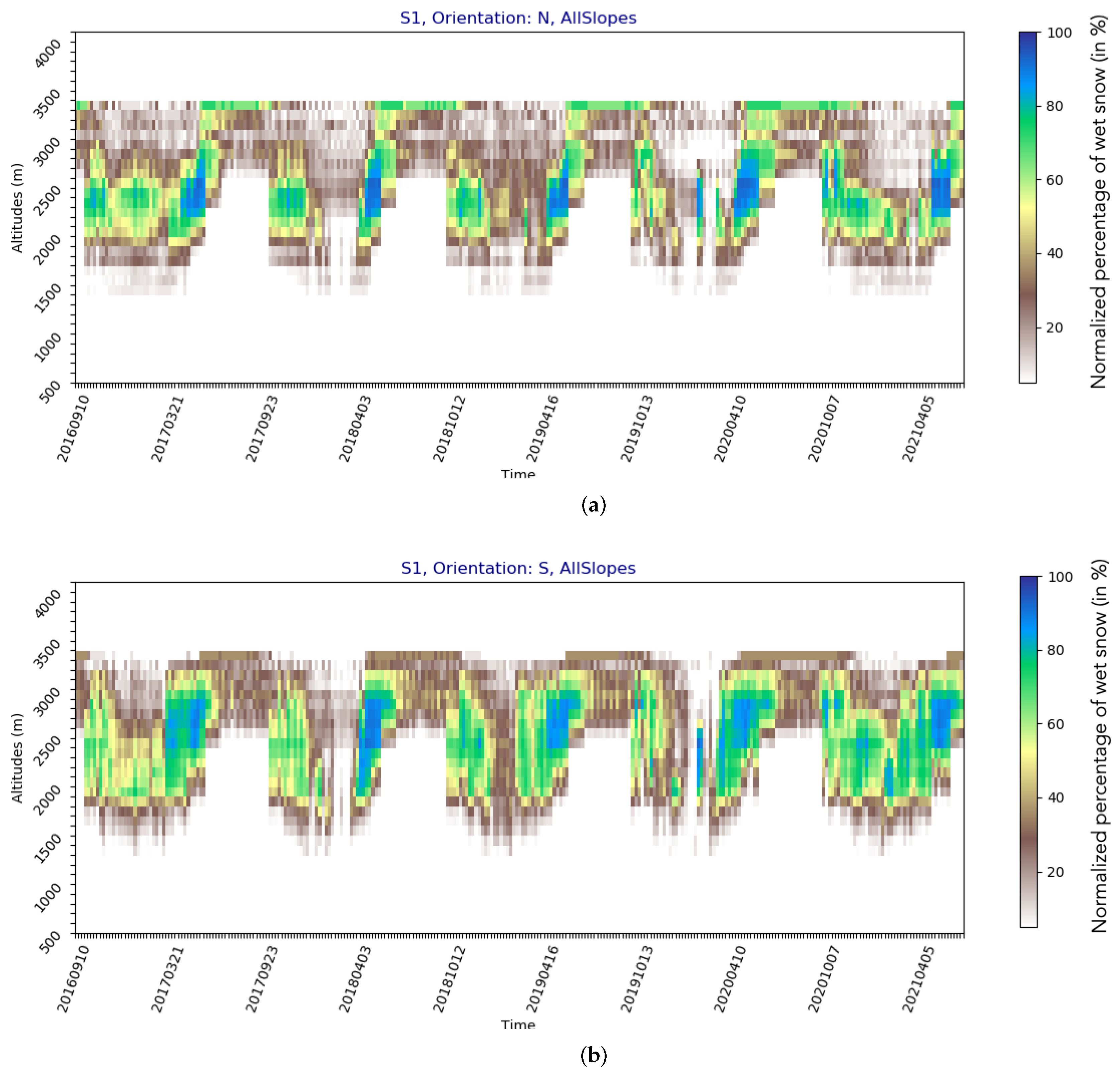
Figure 14 shows Altitude–Time diagrams for northern and southern orientations, respectively, obtained using the normalized percentage of snow-covered pixels by classes of elevation and time for Sentinel-1 descending images.
The computations are shown for the Grandes-Rousses massif. This representation allows to follow the seasonal evolution of wet snow and to monitor altitudes and dates of snow loss. It should be noted that we also observe situations of snow moistening out of the melting periods, which are mainly due to the effects of rain on snow. The winter of 2017–2018 is a perfect example of this with successions of rain-on-snow events during January–February 2018. The meltline graphs illustrate a fairly coherent evolution of wet snow with, in particular, (1) the seasonality of the moistening that takes place between the months of March and April, depending on the season. (2) The extent of wet snow according to altitude is more abundant and occurs earlier in the southern orientation than in the northern orientation.
3.3. Comparisons with Crocus
We compared the satellite products with the reanalyses of the Crocus model. We focused on estimates of snow depth and snow liquid water content. These estimates are available at the scale of the French massifs for our entire study period. The
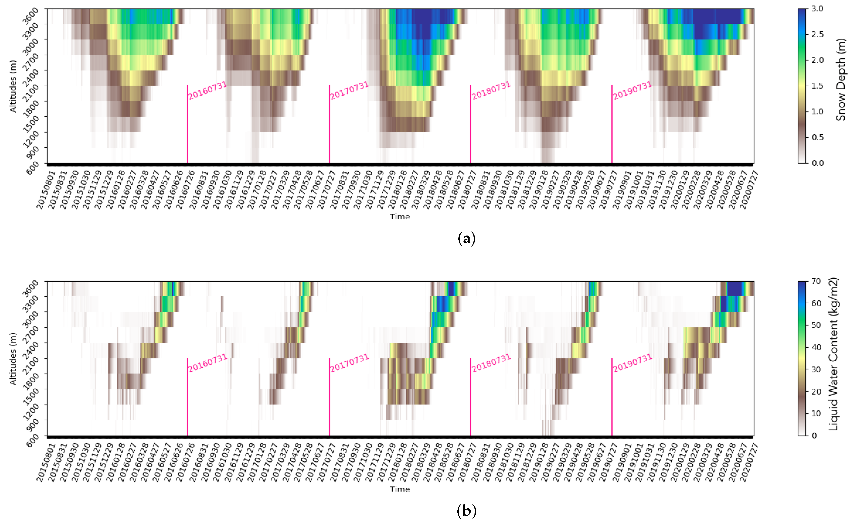
Figure 15 shows the time evolution of snow depth and liquid water content simulated by Crocus at the Grandes-Rousses scale for the northern orientations from 2016 to 2020. The use of Sentinel-1 melt line diagrams makes it easier to compare the satellites with the model.
We do not expect a perfect agreement between observations and the Crocus model, but the goal here is to make a broad comparison between the different products and to outline ways to evaluate the outputs of the models based on the satellite observations.
Figure 15 illustrates the succession of snow seasons as seen by the snow model Crocus. It shows a more intense snow cover in 2018 and 2020 with snow heights exceeding 2 m above 2700 m. These seasons are also marked by a significant amount of wet snow (see Snow Water content graph). This is overall fairly consistent with SWS products, showing abundant wet snow in 2018 and 2020 (see
Figure 14). Differences exist between the model and satellite observations, which is expected. To illustrate this, we will use the example of April 2018, which was marked by an excess of wet snow and which was a relatively cloud-free period providing useful Sentinel-2 images for snow.
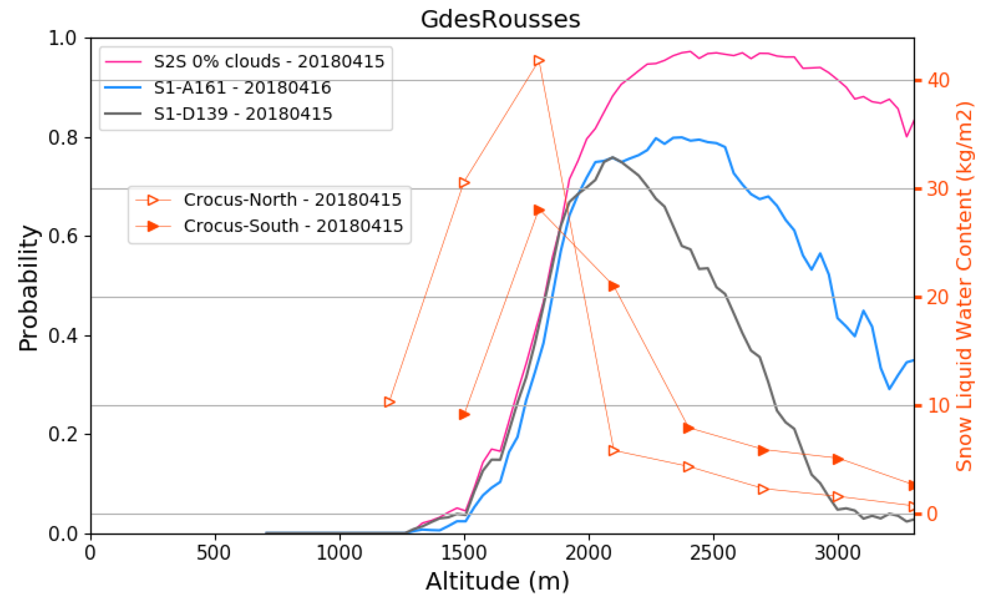
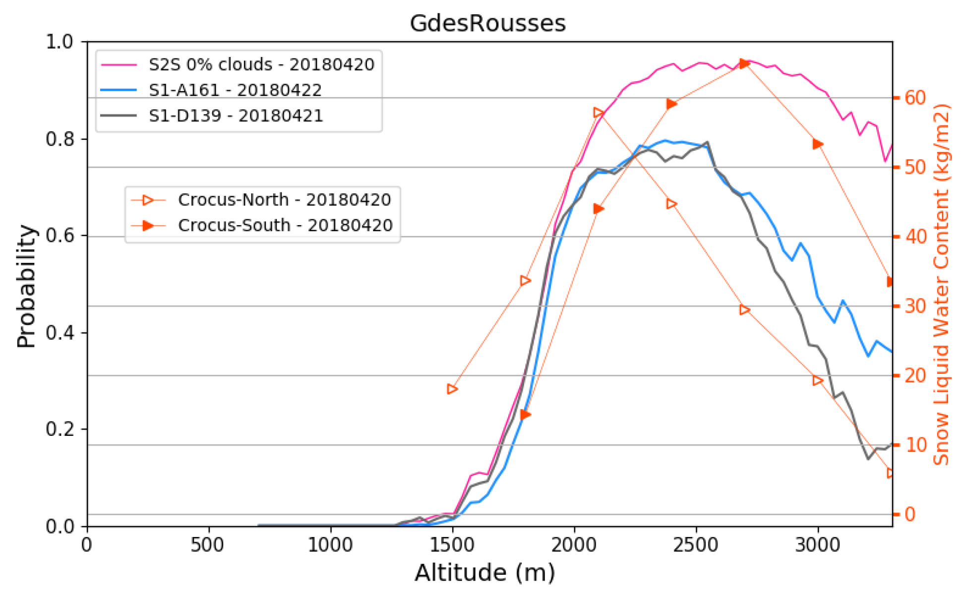
Figure 16 shows the probability curves of snow as function of altitudes for mid-april 2018 obtained from FSC Sentinel-2 product (15 April 2018), SWS ascending (16 April 2018) and descending product (15 April 2018). Snow liquid water simulated by Crocus for the southern and northern orientations are also shown in this figure (orange curves).
Figure 17 and
Figure 18 are similar to
Figure 16 but for dates close to 20 April 2018 and to 25 April 2018, respectively.
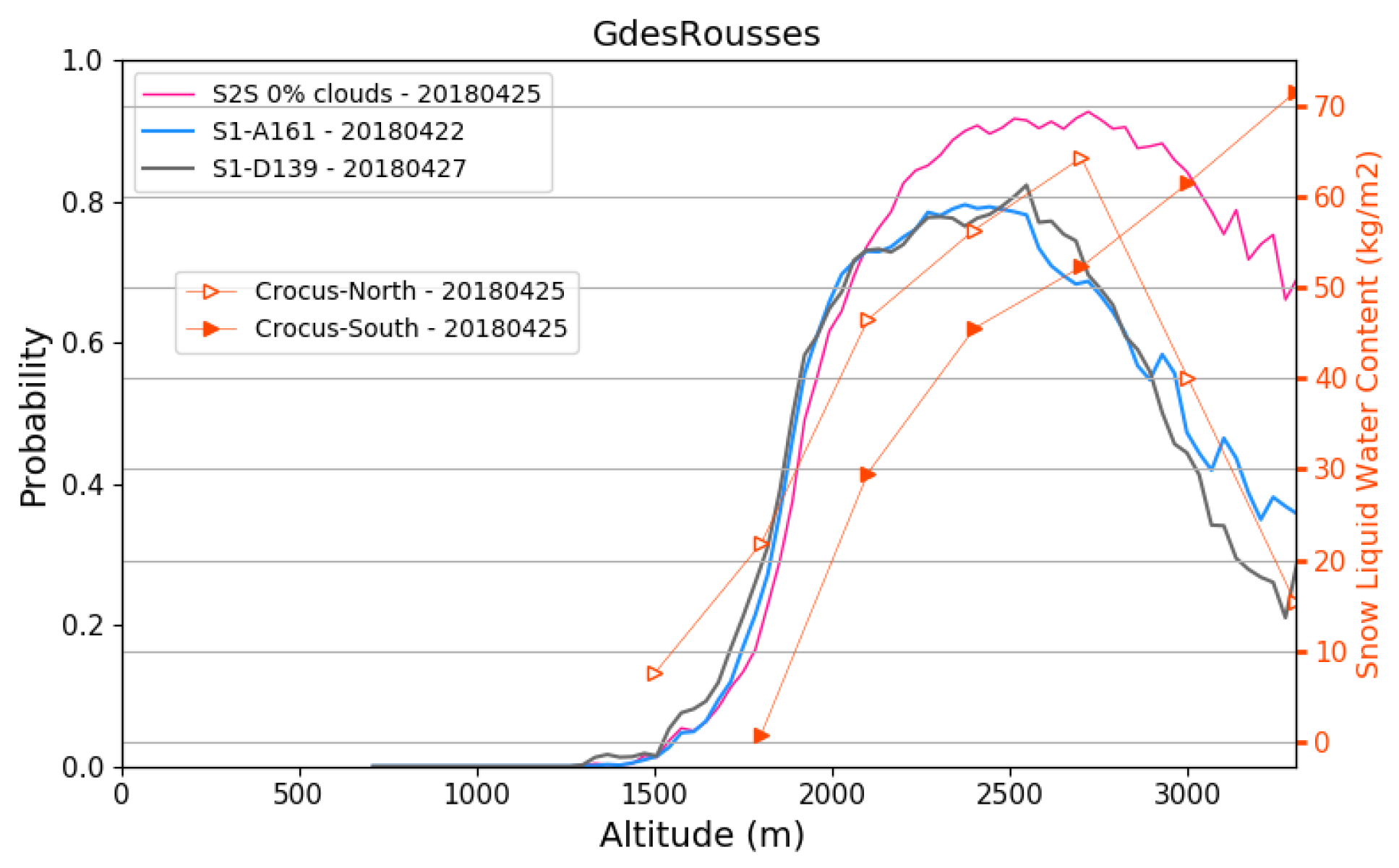
For mid-April, the Crocus model simulates wet snow for elevation ranges from 1000 to 2000 with a maximum snow water content at 1800 m. SWS products show a maximum probability of wet snow at about 2500 m in the afternoon and 2000 m in the early morning. When looking at the 20 April date, Crocus appears to locate wet snow in better agreement with satellite products with a maximum LWC at 2500 m for southern orientations and 2000 m for northern orientations. The morning and evening orbits show a maximum probability of wet snow between 2000 and 2500 m. For 25 April, the model places the maximum of liquid water content in the southern orientation on the very high altitudes and at 2700 m for the northern orientations. The satellites place the maximum probability of wet snow on the interval 2000–2500 m. Comparisons of the snow probability and liquid water content (or snow height, not shown) curves are not straightforward, but they provide us with a general picture of the agreements and disagreements between the different products. This type of diagram can be used as an independent way to evaluate models, especially in a data assimilation context (i.e., to check after assimilation of data if the model is getting closer or further away from the satellite estimates).
4. Discussion and Conclusions
This paper gathers a set of studies undertaken to evaluate the new Copernicus SWS products in mountain terrain. Five successive seasons of data (2017 to 2021) have been studied on a high mountain area in the French Alps. Comparison was made against Sentinel-2 snow fraction products (FSC) and snow reanalyses from the state-of-art snow model Crocus model. We first introduced a new score called PSSP (Probabilistic Score for Satellite Products), which allows to compare very usefully satellite products of different nature and which is particularly adapted for mountain products. We have shown that for periods of melting, the probability curves of snow cover from Sentinel-1 and Sentinel-2 are very close for altitudes below 2000 m with RMS errors below 0.2. At higher altitudes, the RMS errors are higher and this may be explained by the presence of dry snow, which is not detected by the SAR and/or a high cloud cover, which makes the comparison between optical and radar difficult. We have also shown that the probability curves generated in this way make it possible to infer very relevant information on the extent of snow by altitude and on its melting process by combining information from Sentinel-2 and Sentinel-1 (with the morning and evening orbits). It should be noted that the PSSP score makes it possible to compare products or simulations at the scale of an area of interest regardless of their spatial resolution. Moreover, these diagnostics could be refined by calculating probability curves for a given orientation (northern or southern for example).
We calculated the melt lines from SWS products by elevation and orientation using the method described by [
10]. The results show expected variations in wet snow, consistent with seasons and/or rain-on-snow events. The analyses performed show that SWS products can be effectively used to monitor the evolution of wet snow cover at different Sentinel-1 acquisition dates. The graphs also compare favourably with some snowpack seasonal patterns as seen by the Crocus model even though differences do exist between the different data. Comparisons with the Crocus model suggest two avenues of exploitation of SWS products, namely (1) their use to evaluate the outputs of snow models and (2) their potential application as inputs to feed models through data assimilation methods. Studies are underway to systematically compare the snow liquid water content simulations of the Crocus model with the SWS products and to evaluate the points of agreement and disagreement between these databases at the scale of the French Alps. This would allow, among other effects, to better identify potential model biases during melting periods and to implement an adequate evaluation system for the snow model. Other studies are also conducted to assimilate snow and wet snow products from Sentinel-2/Sentinel-1 satellites respectively into the Crocus snow model using an ensemble assimilation chain based on a particle filter approach at a resolution of 250 m [
22].
Some further conclusions can be drawn from this work. The new SWS products from Copernicus appear to be very relevant to study the evolution of wet snow cover in alpine areas. Even if the study was only limited to part of the French Alps, we anticipate a similar quality of products across other mountain areas. However, we have only used SAR data from two relative orbits: relative orbit numbers 161 and 139 for ascending and descending orbits respectively. An inter-comparison study of SWS products from several orbits over a given area would provide additional validation of the product. From our study, different characteristics of the snow cover according to the seasons have been be put forward (regarding the extent of the wet snow for some key dates). The SWS product could therefore be very useful to characterise for each season the beginning of melting as well as the dates and altitudes of snow loss. We also show that the PSSP score is useful to compare satellite products and to evaluate SWS products in particular. Generating snow probability curves by altitude and by successive dates would make possible to monitor snowmelt steps at the scale of a mountain range by exploiting jointly the evening and morning SAR orbits. For instance, an increase of wet snow probabilities with the morning orbit could indicate a generalisation of melting or snow ripening. Comparing the probability curves for total and wet snowfall would provide additional insight into the evolution of the snowpack.
The PSSP score python code (with documentation and test data) will soon be made available to researchers on a code-sharing site and can also be obtained from the corresponding author upon request.
Author Contributions
Research design, F.K. and G.J.; Data analysis, F.K. and G.J. with support from M.F.; Data Preprocessing: F.K., M.F. and F.M.; Result analysis, F.K. and G.J.; Writing-Original Draft Preparation: F.K., G.J. and F.M.; Writing-Review-Editing: F.K., G.J., F.M. and M.F. All authors have read and agreed to the published version of the manuscript.
Funding
This work has been supported by the CNES Tosca (APR SHARE).
Data Availability Statement
Snow products are available from the Copernicus Land Monitoring Service web site
https://land.copernicus.eu, accessed on 1 January 2022. The data, diagrams generated in this article can be obtained upon request to the corresponding author. The PSSP score python code (with documentation and test data) will soon be made available to researchers on a code-sharing site and can also be obtained from the corresponding author upon request.
Acknowledgments
The authors would like to thank the four anonymous reviewers for their helpful comments that helped improve the article. The authors would like to acknowledge the support provided by CNES for preprocessing SAR images using the PEPS facilities, as well as the European Environnement Agency. This study has been conducted using E.U. Copernicus Land Service Information.
Conflicts of Interest
The authors declare no conflict of interest.
Abbreviations
| PSSP | Probabilistic Score for Satellite Products |
| SWS | SAR Wet Snow |
| LWC | Liquid Water Content |
| FSC | Fractional Snow Cover |
| MGRS | Military Grid Reference System |
References
- Stillinger, T.; Roberts, D.A.; Collar, N.M.; Dozier, J. Cloud Masking for Landsat 8 and MODIS Terra Over Snow-Covered Terrain: Error Analysis and Spectral Similarity Between Snow and Cloud. Water Resour. Res. 2019, 55, 6169–6184. [Google Scholar] [CrossRef] [PubMed] [Green Version]
- Xin, Q.; Woodcock, C.E.; Liu, J.; Tan, B.; Melloh, R.A.; Davis, R.E. View angle effects on MODIS snow mapping in forests. Remote Sens. Env. 2012, 118, 50–59. [Google Scholar] [CrossRef] [Green Version]
- Hagolle, O.; Huc, M.; Villa Pascual, D.; Dedieu, G. A Multi-Temporal and Multi-Spectral Method to Estimate Aerosol Optical Thickness over Land, for the Atmospheric Correction of FormoSat-2, LandSat, VENμS and Sentinel-2 Images. Remote Sens. 2015, 7, 2668–2691. [Google Scholar] [CrossRef] [Green Version]
- Nagler, T.; Rott, H. Retrieval of wet snow by means of multitemporal SAR data. IEEE Trans. Geosci. Remote Sens. 2000, 38, 754–765. [Google Scholar] [CrossRef]
- Nagler, T.; Rott, H.; Ripper, E.; Bippus, G.; Hetzenecker, M. Advancements for Snowmelt Monitoring by Means of Sentinel-1 SAR. Remote Sens. 2016, 8, 348. [Google Scholar] [CrossRef] [Green Version]
- Baghdadi, N.; Gauthier, Y.; Bernier, M.; Fortin, J.P. Potential and Limitations of RADARSAT SAR Data for Wet Snow Monitoring. IEEE Trans. Geosci Remote Sens. 2000, 38, 316–320. [Google Scholar]
- Koskinen, J.; Pulliainen, J.; Hallikainen, M. The use of ERS-1 SAR data in snow melt monitoring. IEEE Trans. Geosci. Remote Sens. 1997, 35, 601–610. [Google Scholar] [CrossRef]
- Luojus, K.; Pulliainen, J.; Metsamaki, S.; Hallikainen, M. Snow-Covered Area Estimation Using Satellite Radar Wide-Swath Images. IEEE Trans. Geosci. Remote Sens. 2007, 45, 978–989. [Google Scholar] [CrossRef]
- Marin, C.; Bertoldi, G.; Premier, V.; Callegari, M.; Brida, C.; Hürkamp, K.; Tschiersch, J.; Zebisch, M.; Notarnicola, C. Use of Sentinel-1 radar observations to evaluate snowmelt dynamics in alpine regions. Cryosphere 2020, 14, 935–956. [Google Scholar] [CrossRef] [Green Version]
- Karbou, F.; Veyssière, G.; Coleou, C.; Dufour, A.; Gouttevin, I.; Durand, P.; Gascoin, S.; Grizonnet, M. Monitoring Wet Snow Over an Alpine Region Using Sentinel-1 Observations. Remote Sens. 2021, 13, 381. [Google Scholar] [CrossRef]
- Tsai, Y.L.; Dietz, S.; Oppelt, A.; Kuenzer, N. Remote Sensing of Snow Cover Using Spaceborne SAR: A Review. Remote Sens. 2019, 11, 1456. [Google Scholar] [CrossRef]
- Gascoin, S.; Barrou Dumont, Z.; Deschamps-Berger, C.M.F.; Salgues, G.; López-Moreno, J.; Revuelto, J.; Michon, T.; Schattan, P.; Hagolle, O. Estimating Fractional Snow Cover in Open Terrain from Sentinel-2 Using the Normalized Difference Snow Index. Remote Sens. 2020, 12, 2904. [Google Scholar] [CrossRef]
- Deschamps-Berger, C.; Gascoin, S.; Berthier, E.; Deems, J.; Gutmann, E.; Dehcq, A.; Shean, D.; Dumont, M. Snow depth mapping from stereo satellite imagery in mountainous terrain: Evaluation using airborne laser-scanning data. Cryosphere 2020, 14, 2925–2940. [Google Scholar] [CrossRef]
- Wendleder, A.; Dietz, A.J.; Schork, K. Mapping Snow Cover Extent Using Optical and SAR Data. In Proceedings of the IGARSS 2018—2018 IEEE International Geoscience and Remote Sensing Symposium, Valencia, Spain, 22–27 July 2018; pp. 5104–5107. [Google Scholar] [CrossRef] [Green Version]
- Gascoin, S.; Grizonnet, M.; Bouchet, M.; Salgues, G.; Hagolle, O. Theia Snow collection: High-resolution operational snow cover maps from Sentinel-2 and Landsat-8 data. Earth Syst. Sci. Data 2019, 11, 492–514. [Google Scholar] [CrossRef] [Green Version]
- Brun, E.; Vionnet, V.; Morin, S.; Boone, A.; Martin, E.; Faroux, S.; Le Moigne, P.; Willemet, J.M. Le modèle de manteau neigeux Crocus et ses applications. La Météorologie 2012, 76, 44–54. [Google Scholar] [CrossRef]
- Vionnet, V.; Brun, E.; Morin, S.; Boone, A.; Martin, E.; Faroux, S.; Moigne, P.L.; Willemet, J.M. The detailed snowpack scheme Crocus and its implementation in SURFEX v7.2. Geosci. Model. Dev. 2012, 5, 773–791. [Google Scholar] [CrossRef] [Green Version]
- Decharme, B.; Boone, A.; Delire, C.; Noilhan, J. Local evaluation of the Interaction between Soil Biosphere Atmosphere soil multilayer diffusion scheme using four pedotransfer functions. J. Geophys. Res. 2011, 116, D20126. [Google Scholar] [CrossRef]
- Masson, V.; Le Moigne, P.; Martin, E.; Faroux, S.; Alias, A.; Alkama, R.; Belamari, S.; Barbu, A.; Boone, A.; Bouyssel, F.; et al. The SURFEXv7.2 land and ocean surface platform for coupled or offline simulation of Earth surface variables and fluxes. Geosci. Model Dev. 2013, 6, 929–960. [Google Scholar] [CrossRef] [Green Version]
- Vernay, M.; Lafaysse, M.; Monteiro, D.; Hagenmuller, P.; Nheili, R.; Samacoïts, R.; Verfaillie, D.; Morin, S. The S2M meteorological and snow cover reanalysis over the French mountainous areas: Description and evaluation (1958–2021). Earth Syst. Sci. Data 2022, 14, 1707–1733. [Google Scholar] [CrossRef]
- Durand, Y.; Brun, E.; Mérindol, L.; Guyomarc’h, G.; Lesaffre, B.; Martin, E. A meteorological estimation of relevant parameters for snow models. Ann. Glaciol. 1993, 18, 65–71. [Google Scholar] [CrossRef]
- Cap, E.; Karbou, F.; Lafaysse, M.; Fructus, M. Towards the assimilation of snow products derived from Sentinel-1/Sentinel-2 in the Crocus snow evolution model. In Proceedings of the ESA Living Planet Symposium, Bonn, Germany, 23–27 May 2022. [Google Scholar]
Figure 1.
Location of the study area.
Figure 1.
Location of the study area.
Figure 2.
Maps of Snow cover maps derived from the Sentinel-2 Fractional Snow Cover products on tile 31TGL derived as of (a) 15 April 2018 (b) 20 April 2018 and (c) 25 April 2018.
Figure 2.
Maps of Snow cover maps derived from the Sentinel-2 Fractional Snow Cover products on tile 31TGL derived as of (a) 15 April 2018 (b) 20 April 2018 and (c) 25 April 2018.
Figure 3.
Maps of Sentinel-1 SWS wet snow products derived from the ascending orbit A161 as of (a) 16 April 2018 and (b) 22 April 2018.
Figure 3.
Maps of Sentinel-1 SWS wet snow products derived from the ascending orbit A161 as of (a) 16 April 2018 and (b) 22 April 2018.
Figure 4.
Maps of SWS Sentinel-1 wet snow products from the descending orbit D139 as of (a) 15 April 2018 (b) 21 April 2018 and (c) 27 April 2018.
Figure 4.
Maps of SWS Sentinel-1 wet snow products from the descending orbit D139 as of (a) 15 April 2018 (b) 21 April 2018 and (c) 27 April 2018.
Figure 5.
Probability curves describing the occurrence of snow by altitudes at the scale of the Grandes Rousses massif obtained for three successive Sentinel-2 dates (pink curves): 15 April 2018, 20 April 2018 and 25 April 2018, for which no cloud was recorded over the Grandes-Rousses massif. The figure also shows the obtained snow probability curves from SWS products for Sentinel-1 ascending scenes observed on 16 April 2018 and 22 April 2018 (blue curves) and for Sentinel-1 descending scenes observed on 15 April 2018, 21 April 2018 and 27 April 2018 (Gray curves).
Figure 6.
RMS errors for different dates of Sentinel-2 observations (April–May). At these dates, SWS products from ascending orbit closest in time to S2 are selected. The results are shown by altitude range (blue squares: 0–2000 m, pink squares: 2000–2500 m, orange squares: 2500–3000 m and yellow squares: >3000 m).
Figure 7.
Same as
Figure 6 but for the descending orbit.
Figure 7.
Same as
Figure 6 but for the descending orbit.
Figure 8.
Cloud rates for selected Sentinel-2 observations (April–May). The results are shown by altitude range (blue squares: 0–2000 m, pink squares: 2000–2500 m, orange squares: 2500–3000 m and yellow squares: >3000 m).
Figure 8.
Cloud rates for selected Sentinel-2 observations (April–May). The results are shown by altitude range (blue squares: 0–2000 m, pink squares: 2000–2500 m, orange squares: 2500–3000 m and yellow squares: >3000 m).
Figure 9.
Sentinel-1 wet snow meltlines from the descending orbit D139 for spring 2017: 15 March 2017, 14 April 2017 and 26 April 2017.
Figure 9.
Sentinel-1 wet snow meltlines from the descending orbit D139 for spring 2017: 15 March 2017, 14 April 2017 and 26 April 2017.
Figure 10.
Same as
Figure 9 but for spring 2018: 15 April 2018, 21 April 2018 and 27 April 2018.
Figure 10.
Same as
Figure 9 but for spring 2018: 15 April 2018, 21 April 2018 and 27 April 2018.
Figure 11.
Same as
Figure 9 but for spring 2019: 17 March 2019, 16 April 2019 and 28 April 2019.
Figure 11.
Same as
Figure 9 but for spring 2019: 17 March 2019, 16 April 2019 and 28 April 2019.
Figure 12.
Same as
Figure 9 but for spring 2020: 17 March 2020, 16 April 2020 and 27 April 2020.
Figure 12.
Same as
Figure 9 but for spring 2020: 17 March 2020, 16 April 2020 and 27 April 2020.
Figure 13.
Same as
Figure 9 but for spring 2021: (
a) 18 March 2021 (
b) 17 April 2021 and (
c) 29 April 2021.
Figure 13.
Same as
Figure 9 but for spring 2021: (
a) 18 March 2021 (
b) 17 April 2021 and (
c) 29 April 2021.
Figure 14.
Altitude–Time diagram with the normalized percentage of wet snow-covered pixels by classes of elevation and time for Sentinel-1 descending SWS products for the Grandes-Rousses massif. Results are given for (a) northern and (b) southern orientations, respectively.
Figure 14.
Altitude–Time diagram with the normalized percentage of wet snow-covered pixels by classes of elevation and time for Sentinel-1 descending SWS products for the Grandes-Rousses massif. Results are given for (a) northern and (b) southern orientations, respectively.
Figure 15.
Time evolution of (a) snow depth (in meters) and (b) liquid water content (in kg/m2) simulated by Crocus at the Grandes-Rousses scale for the northern orientations from 2017 to 2021.
Figure 15.
Time evolution of (a) snow depth (in meters) and (b) liquid water content (in kg/m2) simulated by Crocus at the Grandes-Rousses scale for the northern orientations from 2017 to 2021.
Figure 16.
Snow probability curves as function of altitudes for mid-april 2018 obtained from FSC Sentinel-2 product (15 April 2018, pink curve), SWS ascending (16 April 2018, blue curve) and descending product (15 April 2018, grey curve). Snow liquid water simulated by Crocus for the southern and northern orientations are also shown in this figure (orange curves).
Figure 17.
Same as
Figure 17 but for dates close to 20 April 2018.
Figure 17.
Same as
Figure 17 but for dates close to 20 April 2018.
Figure 18.
Same as
Figure 17 but for dates close to 25 April 2018.
Figure 18.
Same as
Figure 17 but for dates close to 25 April 2018.
| Publisher’s Note: MDPI stays neutral with regard to jurisdictional claims in published maps and institutional affiliations. |
© 2022 by the authors. Licensee MDPI, Basel, Switzerland. This article is an open access article distributed under the terms and conditions of the Creative Commons Attribution (CC BY) license (https://creativecommons.org/licenses/by/4.0/).


