Updated Understanding of the Thompson River Valley Landslides Kinematics Using Satellite InSAR

Abstract

The Thompson River valley is one of the most important transportation corridors in western Canada as it hosts two important railways. This valley has experienced several historical landslide events, many of them along a 10 km section south of the town of Ashcroft. Six of these landslides, showing varying states of activity, were selected for analysis in this paper, as these have the potential for the biggest impact on the railways. The subsurface interpretation of these landslides is combined with satellite InSAR data from May 2015 to May 2017 to enhance the current understanding of the landslide kinematics. Two InSAR orientations are combined geometrically with the assumption that the horizontal component of landslide movement is parallel to the slope azimuth, which provides a practicable approach to approximate landslide displacement vectors. The results classify these landslides as very slow-moving. The maximum velocities recorded are 29, 35, 26, 64, 18, and 52 mm/year for the Goddard, North, South, South extension, Barnard, and Redhill landslides, respectively. All landslides except the Redhill landslide show near-horizontal movements near the toe, with increasing vertical components as measurements approach the back scarp. This confirms that kinematics include rotational and compound mechanisms.

1. Introduction

Landslides are known as a natural phenomenon that poses risks to infrastructure and lives all around the world. Many cases of landslides have been reported in Canada, which have caused many life losses and damage to infrastructure [1,2,3,4]. Hundreds of fatalities and millions of dollars in costs caused by landslides have been recorded in Canada since 1771 [5]. A recent report confirmed four fatalities as a consequence of a landslide on British Columbia’s Highway 99 in November 2021 (Simon Little, Global News, 20 November 2021).

Technical and economic challenges of stabilization or avoidance of landslides in susceptible areas mean that the identification of landslides and monitoring terrain movement is the most efficient risk management tool when combined with warning and action plans. Furthermore, it can inform maintenance requirements for key infrastructures such as roads and railway tracks. Monitoring is commonly employed as part of early warning systems [6,7,8]. Furthermore, monitoring and understanding landslides have become even more important because of climate change effects on landslide activity, for example, due to the acceleration of glacier melting, which is expected to increase landslide activity in northern regions in Canada [5]. Remote landslide monitoring can be used for specific landslides or in large areas to increase the understanding of landslide kinematics and triggers, and to improve landslide risk management strategies [9,10,11,12,13,14].

This paper presents an updated understanding of landslide kinematics using satellite InSAR for six active landslides along the Thompson River Valley in British Columbia, Canada. These landslides are located along a 10 km section south of the town of Ashcroft. Some of these landslides have been studied by a number of researchers [6,7,8,15,16,17,18,19]. In this paper, an update on landslides’ kinematics is presented based on the interpreted stratigraphy in the research area and InSAR monitoring data between May 2015 and May 2017 [6,16,18,19,20,21,22].

To provide a practicable approach to approximate landslide displacement vectors, we employ a combination of the geometry of two InSAR orientations, and the assumed horizontal movement as parallel to the average slope azimuth of each sector of each landslide. This approach was validated for the area matter of this paper in Soltanieh et al., 2022, on the Ripley landslide, which has a long history of monitoring [8].

1.1. Landslide Remote Sensing and Satellite InSAR

New observation technologies help geotechnical engineers to investigate the terrain’s movement continuously. Many tools such as remote sensing, GPS monitoring, geophysical imaging, and geotechnical surveys are employed for landslide characterization [23]. Interferometric Synthetic Aperture Radar (InSAR), Light Detection and Ranging (LiDAR), and Unmanned Aerial Vehicle (UAV) photogrammetry are some examples of the remote sensing techniques that are employed to monitor cut slopes or natural slopes in routine geohazard monitoring programs. Using these remote sensing methods, engineers and researchers are able to investigate landslide kinematics on large areas with high spatial resolution, when compared with in-place instruments such as slope inclinometers or survey monuments [24].

Radar satellites can carry sensors for Interferometric Synthetic Aperture Radar (InSAR) monitoring, where the relative change in the distance between the radar and ground surface can be calculated by using wavelength information. These abilities make InSAR a robust method in many applications to detect surface displacements of crustal deformation, glacier motion and landslides [25].

Interferometric synthetic aperture radar (InSAR) has been used in many worldwide applications to detect surface displacements of crustal deformation, glacier motion, infrastructure displacement, and landslides in recent decades [26,27,28,29,30,31,32,33,34,35,36,37,38,39].

The accuracy of satellite InSAR provides many advantages for monitoring landslide activity, particularly in remote areas where installation and using in-place ground monitoring instruments is challenging both economically and technically. Despite extensive applications of satellite InSAR for monitoring landslides in the recent 30 years, using this method is still challenging for rapid landslides due to gaps between two consecutive data acquisitions and the potential high acceleration of some landslides. There are also other challenges to this technique, such as atmospheric noise, vegetation cover, and seasonal effects such as rainfall or snow cover [5]. Even with these limitations, satellite InSAR has become an effective and reliable method for many applications [40].

Using satellite InSAR data together with other monitoring information such as precipitation or groundwater fluctuation data can allow for a robust understanding of landslide mechanisms and possible triggers, and this method can be employed effectively to measure the displacement of slow or extremely slow-moving slopes as well as capture the initiation of acceleration [16].

Although satellite revisiting times (now approximately 3 days to 1 week) limit the temporal resolution of InSAR monitoring, the good resolution of InSAR monitoring systems (sub-cm/year) makes it a very useful tool for monitoring landslides [16].

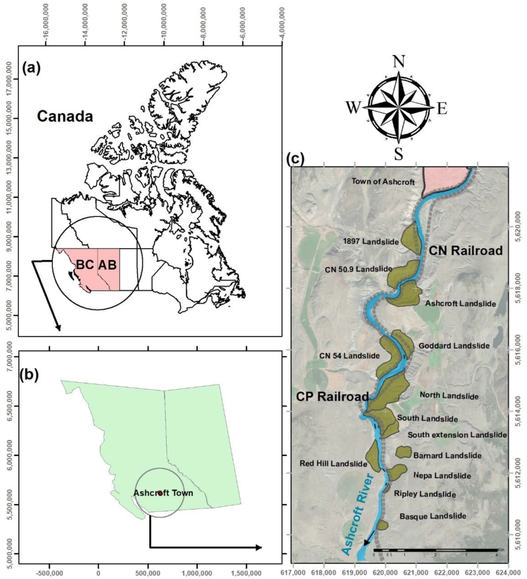
1.2. The Thompson River Valley Landslides South of Ashcroft

The Thompson River valley, south of the town of Ashcroft in British Colombia Canada, is host to the Canadian Pacific Railway (CP) and Canadian National Railway (CN) main lines connecting the port of Vancouver and the rest of Canada. This corridor is therefore very important for the Canadian economy [4]. The importance of this corridor led Natural Resources Canada (NRCAN), the Geological Survey of Canada (GSC), and Transport Canada (TC), in partnership with both CN and CP, the University of Alberta, and Queen’s University, to monitor the Thompson River valley along a 10 km section south of the town of Ashcroft, where up to 14 landslides have been identified [16,41]. A collaboration with the TRE ALTAMIRA CLS Group (TRE) provided the satellite InSAR data used in this study.

River erosion cut the Thompson River valley, which was formed by a series of glaciations. Valley slopes in the glacial sediments are between 75 and 125 m high and their angles from toe to valley crest vary between 15 and 30 degrees. Multiple glacial advance and retreat intervals in the Pleistocene period filled the valley with a complex sequence of a wide range of deposits, from poorly sorted sand and gravel to rhythmically interbedded silt and clay. Triassic and Jurassic volcanic and sedimentary rocks formed the local bedrock in this area [7,41,42,43]. The southward flowing Thompson River cut 150 m of glacial deposited sediments leading to the formation of several landslides [41]. The presence of a weak silt and clay layer has been identified as the main geomorphological feature for the formation of these landslides, which are characterized by multiple graben and horst features as well as steep internal shear and basal through-going surfaces along these weak materials [7,19,42]. The residual shear strengths in these weak silt and clay layers are characterized by friction angles between 9 and 16 degrees [17,41,44]. Figure 1 shows the location of Thompson River valley and the extent of 12 of the 14 landslides identified in this valley. The volumes of the landslides in Thompson River valley vary between 0.75 million cubic meters for the Ripley landslide and more than 15 million cubic meters for the North Landslide. Displacement rates range between 10 mm/year (extremely Slow) and up to 50 mm/s (very rapid), historically, in some areas [7].

2. Materials and Methods

2.1. Satellite InSAR Displacement Data

The satellite InSAR data were captured by the Sentinel 1 project and processed by TRE. Satellite images used in this study were collected between 3 November 2014 and 17 March 2018 for the ascending orbit, and between 6 November 2014 and 1 April 2018 for the descending orbit. The line of sight (LOS) displacement, which is the projection of the real surface displacement on the visual line between the radar’s sensor installed on the satellite and the area monitored, corresponds to overlapping timelines for each geometry (ascending and descending). The ascending geometry data correspond to data captured when the satellite moves from south to north and, given the satellite sensor positioning, captured images look towards the east. The descending geometry corresponds to data captured when the satellite travels from north to south and looks west. These geometries are defined by the angle between the LOS and the vertical plane—theta (θ)—and the angle between the satellite’s orbit and the geographic north—delta (δ). LOS angles are shown in

Table 1. Satellite viewing (LOS) angles for the Sentinel and Radarsat-2 imagery.

Satellite	Orbit Geometry	Track	Sensor Mode	Symbol	Angle (degree)
Sentinel	Ascending	64	IW	θ δ	38.66 11.33
Sentinel	Descending	115	IW	θ δ	44.29 7.79

.

Figure 2 shows a schematic of the geometry for both Sentinel ascending and descending orbits.

InSAR displacement data correspond to scatterers, including those on structures and natural features such as rock outcrops or exposed ground, which are likely stable (permanent scatterers or PS) and distributed scatterers (DS) on large areas (up to hundreds of square meters) identified from exposed ground. Although each DS is represented by a point (location), these points actually correspond to non-point features (areas). A summary of the data properties collected by the Sentinel satellite is presented in

Table 2. Details of the processed satellite InSAR data.

Radar Data Information
Satellite	Sentinel 1	Sentinel 1
Acquisition Geometry	Ascending	Descending
Period Covered by Imagery	3 November 2014 to 17 March 2018	6 November 2014 to 1 April 2018
No. of Processed Images	51	59
Coordinate System	WGS 1984	WGS 1984
Area of Interest	869.2 ${\mathrm{Km}}^2$	869.2 ${\mathrm{Km}}^2$
Number of PS + DS	194,083 (112,343 PS, 81,740 DS)	178,396 (89,510 PS, 88,886 DS)
Sensor Mode	IW	IW
Image Resolution	20 m × 5 m	20 m × 5 m

.

The processing technique for InSAR ground displacement calculations used by TRE corresponds to the SqueeSAR method and it incorporates PSInSAR processing [45]. InSAR data are impacted by topographic distortions, atmospheric effects, and other sources of noise. The Differential InSAR (DInSAR) can be employed to identify and quantify ground movement by removing topographical effects using a DEM of the area of interest. The accuracy of this method is relatively low (cm scale). The atmospheric noise can be removed by the Permanent Scatterer SAR Interferometry (PSInSAR) method, which is an advanced form of DInSAR. The accuracy of this method is higher than DInSAR (milimetre accuracy) and a history of both linear and non-linear ground motion can be detected. The PSInSAR was developed to detect the motion of PS data. The algorithms developed by TRE include the use of SqueeSAR, which incorporates PSInSAR to also process the signals reflected from DS areas. This algorithm effectively reduces noise in data and keeps the accuracy in the millimetre scale [46].

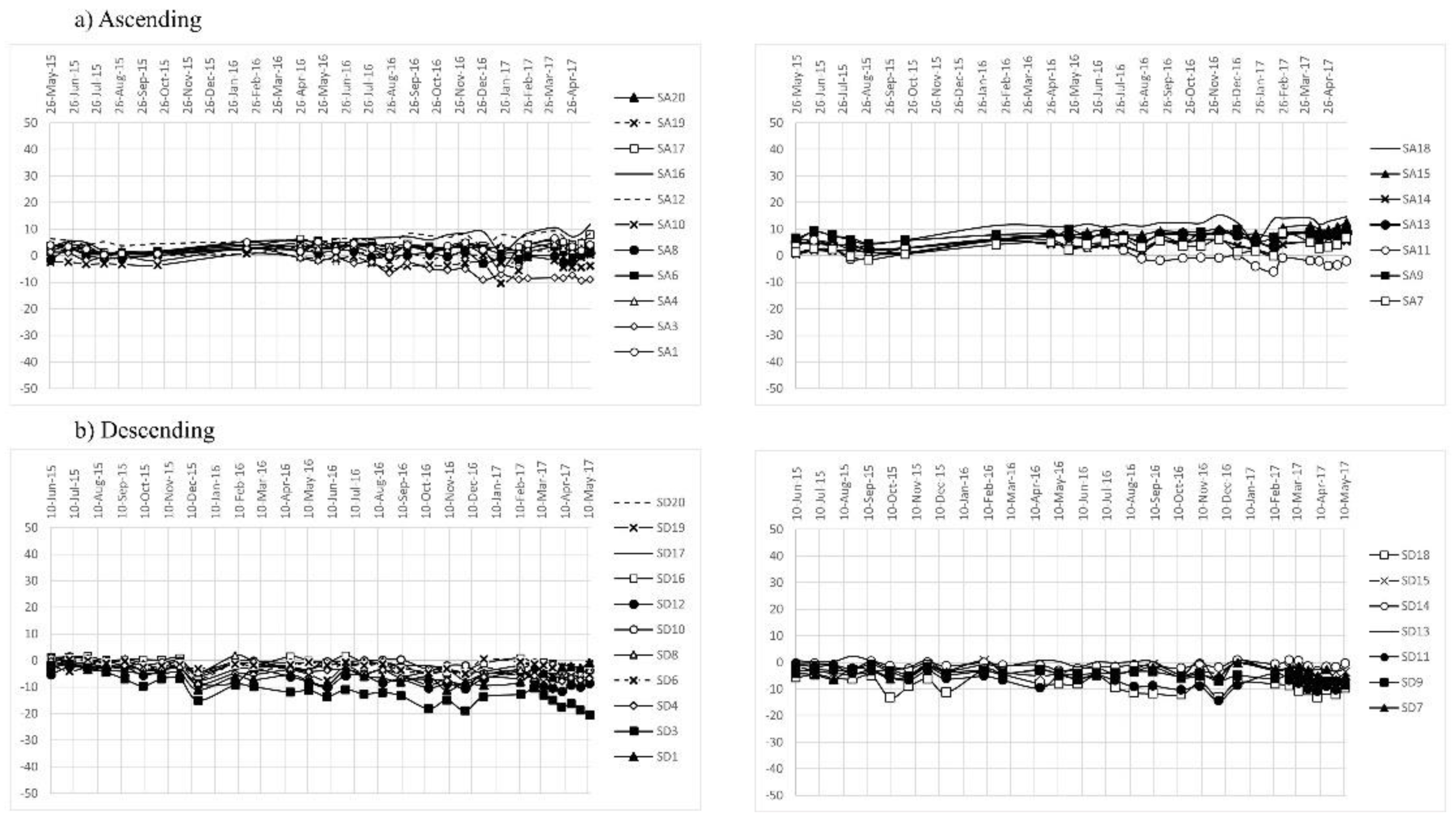
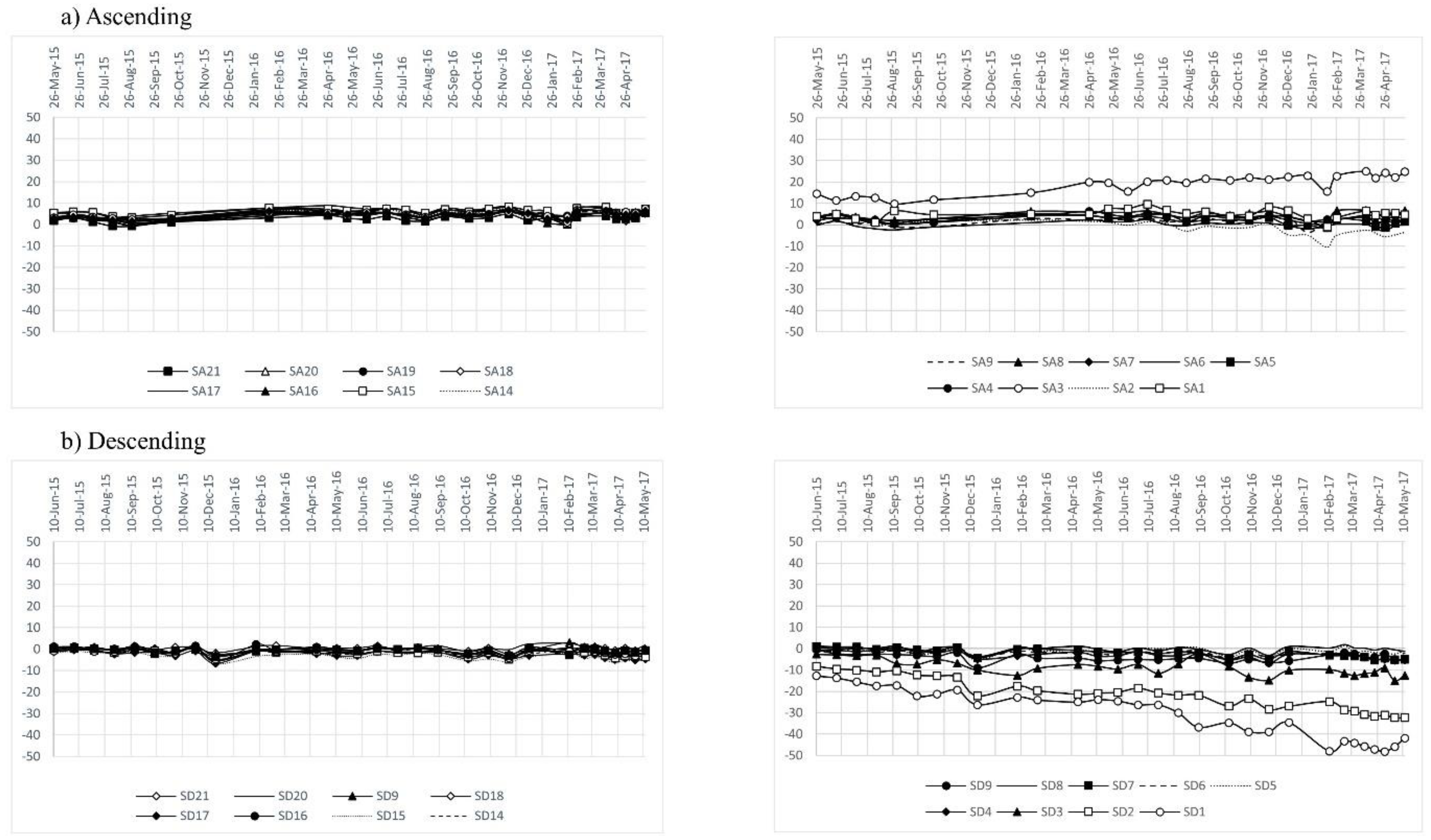
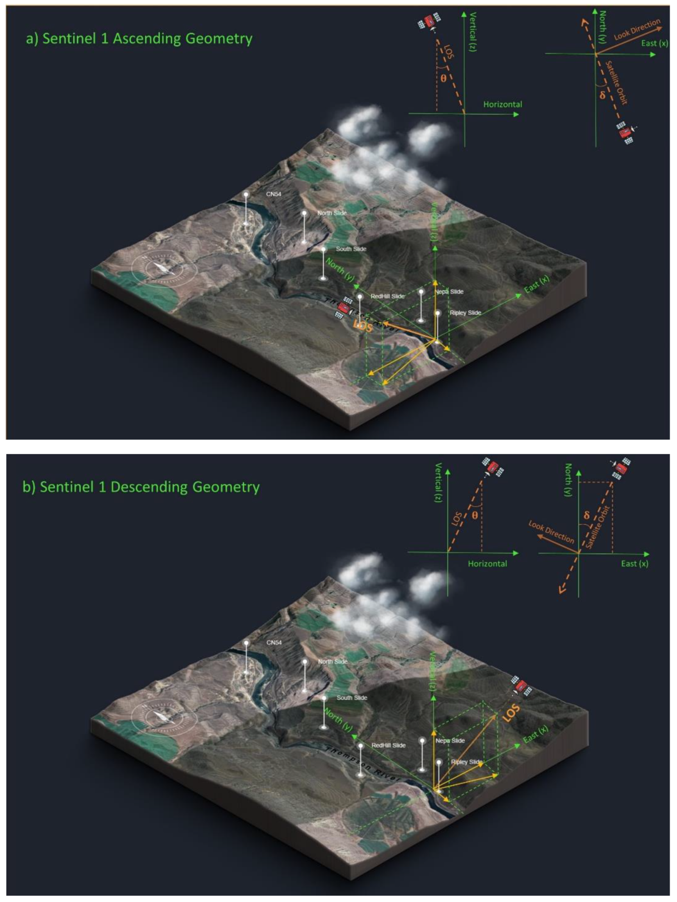
2.2. Surface Ground Displacement Calculations Based on InSAR LOS Displacements

The projection of true landslide surface displacement in each LOS direction is equal to the change in LOS distance between two different readings. In theory, three LOS displacements are needed to fully resolve the true landslide surface displacement. However, LOS displacements correspond to different acquisition times and different data point locations between the ascending and descending geometries. Therefore, the solution requires adopting some spatial and temporal averaging of data. Furthermore, the predominantly north–south direction of the satellite orbit precludes the optimal use of the north component of LOS displacements. The processes followed in this paper are presented and validated for a landslide in this area by Soltanieh and Macciotta [47].

The true ground displacement is called the “Real vector” and is represented by a bold R to show it is a vector. The north–south displacement components are not considered reliable because the given orbits are sub-parallel to the north–south direction. Assuming R is parallel to the downslope direction (both azimuth and inclination) is a common assumption for landslide InSAR interpretation [10]. In this paper, it is assumed that the horizontal component of R is parallel to the slope azimuth (average slope azimuth in the area of analysis). Therefore, the unit vector of the horizontal component of R can be calculated using the topography of the area. A digital elevation model (DEM) of the Thompson River valley was used in ArcMap [48] to calculate the average azimuth of the vector normal to the slope. Considering the vertical component of R as unknown, the assumption of the horizontal component direction, and projecting R to the LOS unit vectors based on the satellite geometries for both satellite orbits, allows us to calculate an approximation for all components of R. The following process is presented in Soltanieh and Macciotta [47].

Unit vectors of LOS are denoted as ${\mathit{S}}_a$ for Sentinel ascending and ${\mathit{S}}_d$ for Sentinel descending. The projections of R in these directions are the measured LOS displacements, denoted by vectors ${\mathit{P}}_a and {\mathit{P}}_d$, respectively. Each of these vectors has a scalar magnitude, $M_a and M_d$, respectively. Equation (1) presents the expression for ${\mathit{P}}_i$, where i represents the ascending or descending orbit.

$${\mathit{P}}_i=\left(R·{\mathit{S}}_i\right) {\mathit{S}}_i=M_i {\mathit{S}}_i$$

(1)

The components of vector R are denoted as (x,y,z), where the components of the unit vectors of the LOS are denoted as ${\mathit{S}}_i=\left(e,n,u\right)$. Calculating the LOS unit vectors requires the angles between the LOS, the vertical plane, and the azimuth from Table 2 (Equations (2)–(4)).

$$u=\cos \theta$$

(2)

$$e=\sin \theta .\sin \delta$$

(3)

$$n=\sin \theta .\cos \delta$$

(4)

The coordinate system adopted corresponds to (East, North, Up). The sign u is positive and the sign n is negative for both orbits’ LoS. the sign e is negative for the ascending orbit, and it is positive for the descending orbit. The unit vectors are calculated following:

$${\mathit{S}}_a=\left(-0.613,-0.123,0.781\right)$$

(5)

$${\mathit{S}}_d=\left(0.692,-0.095,0.716\right)$$

(6)

Replacing Equations (5) and (6) with Equation (1) and solving for $M_a and M_d$ result in the measured LOS displacements in terms of the components of R (Equations (7) and (8)).

$$-0.6-3\mathrm{x}-0.123\mathrm{y}+0.781\mathrm{z}=M_a$$

(7)

$$0.6-2\mathrm{x}-0.095\mathrm{y}+0.716\mathrm{z}=M_d$$

(8)

The third equation required to calculate the components of R corresponds to the assumption that the total horizontal vector component of R is parallel to the slope’s azimuth in the area of measurement (α):

$$\frac{x}{y}=\tan \alpha$$

(9)

Equations (7)–(9) are a system of three equations and three unknowns for estimating R.

It was mentioned that the spatial and temporal inconsistency between ascending and descending InSAR data required spatial and temporal averaging. Spatial averaging considered segmentation of the landslides that balanced data density (e.g., availability of both ascending and descending orbits’ data) and covered different portions of the landslide to allow kinematic interpretation. This decision-making process was performed qualitatively and based on the experience of the authors from previous research [47]. Figure 3 shows the data density for all investigated landslides. It is shown that almost all of these areas contain more than one scatterer of each orbit, and the average of these scatterers is used as representative of LOS displacements for the area.

To minimize the influence of asynchronous data points between orbits, relatively long periods of time for calculating average R (annual basis) were adopted, which led to differences of only a few days in the data for both orbits. This was considered adequate and was tested for the Ripley landslide [47]. The movement rate of the Ripley landslide had been reported at approximately 150 mm/year (0.4 mm/day), suggesting that asynchronous measurements of less than two weeks for a total period of analysis of two years (26 May 2015 to 21 May 2017 for the ascending orbit and 10 June 2015 to 12 May 2017 for the descending orbit, the time span used in this paper) would represent approximately 2% error.

3. Results

This section presents the LOS ground displacements measured by Sentinel 1 in both orientations, and the calculated R for each landslide sector. R is presented as the horizontal component in the plan view, and as the resultant vector of vertical and horizontal components in section views. The cross-sections were developed based on the topography of the area and the stratigraphy for the landslides in Eshgahrian [19,49]. The stratigraphy for the Redhill landslide was estimated based on information about adjacent landslides.

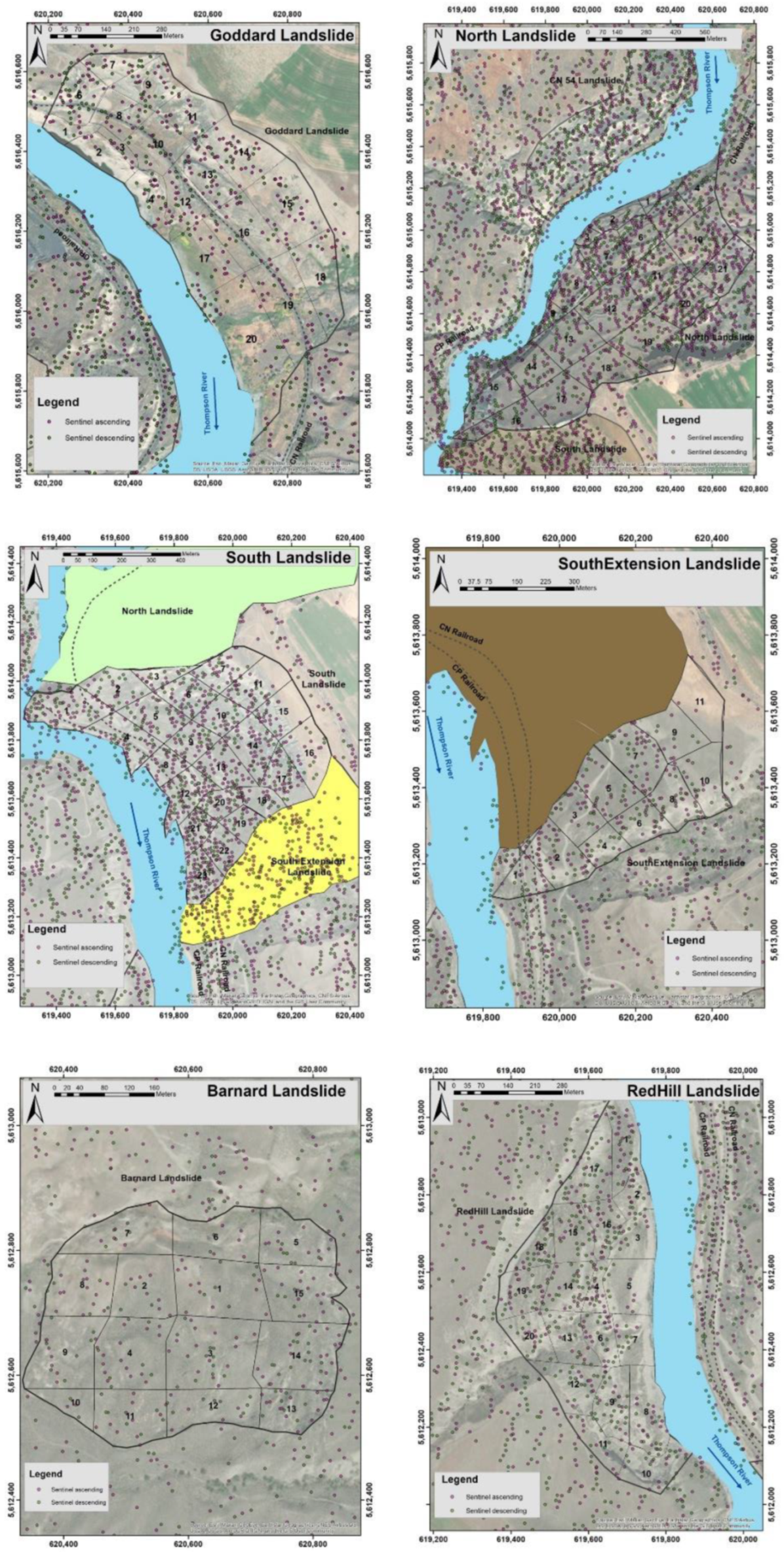
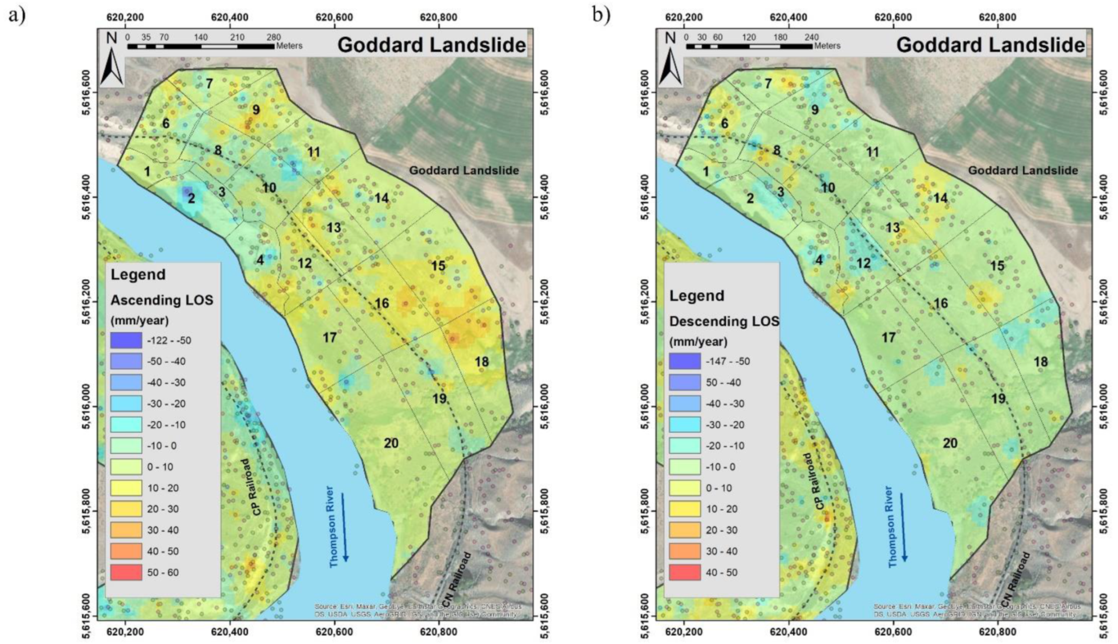
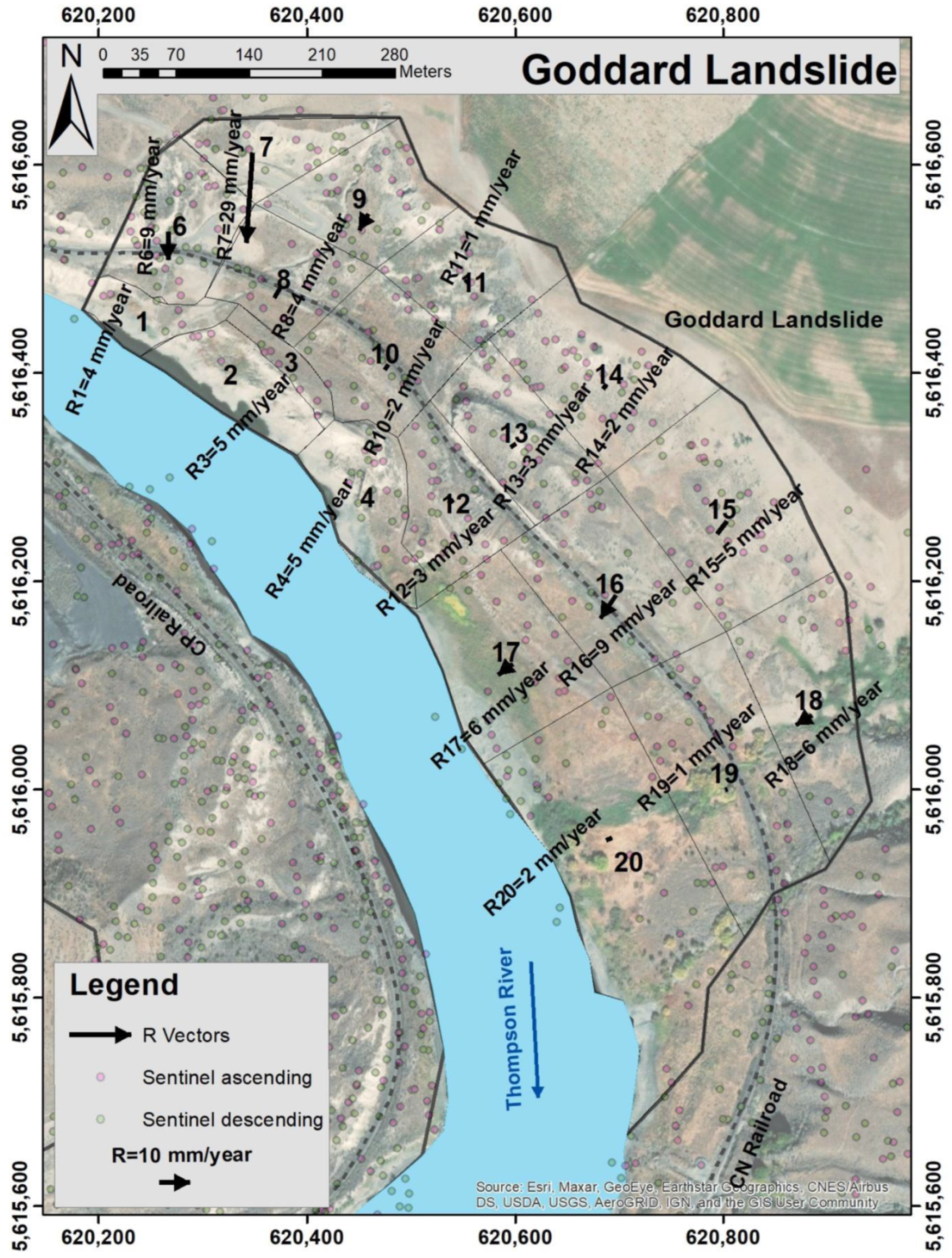
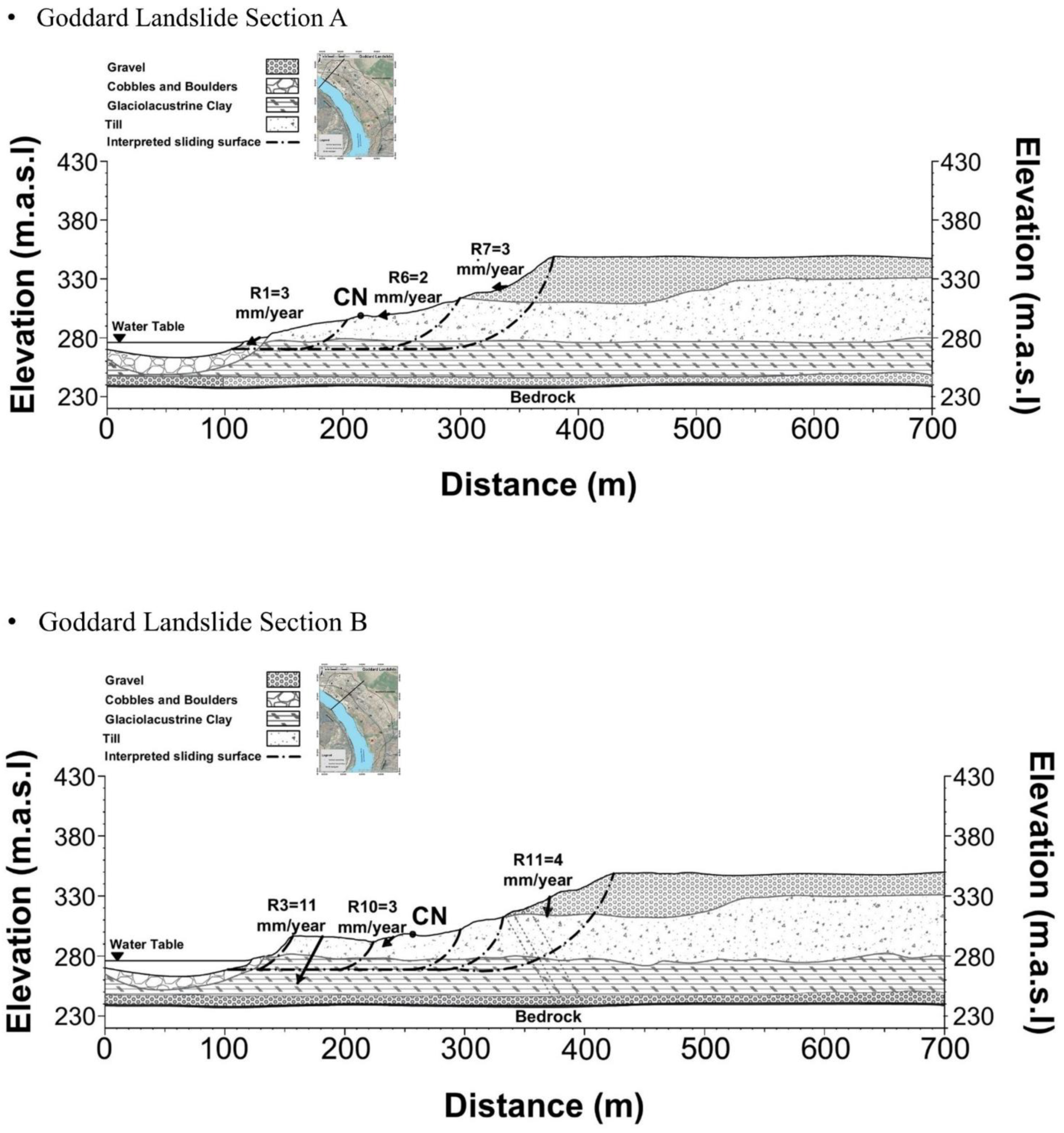
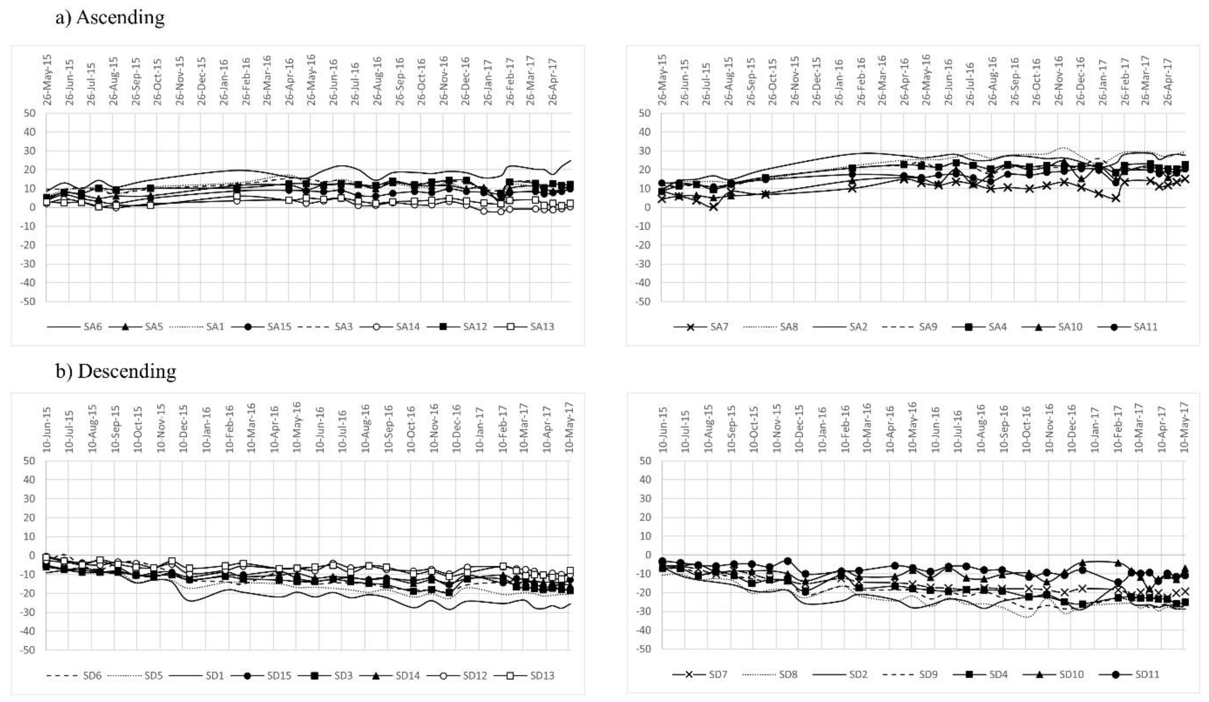
3.1. Goddard Landslide

The magnitudes of recorded cumulative LOS displacement at the end of the selected timelines for both orbits (26 May 2017 and for the ascending orbit and 12 May 2017 for the descending orbit) are shown in Figure 4 for each sector of the landslide. Landslide displacement is minor in most places on the Goddard landslide. The LOS displacement rates are less than 10 mm/year in most sectors of the landslide during the period of analysis.

Figure 5 shows the cumulative average LOS for each sector of the landslide. The average cumulative LOS displacement does not exceed 20 mm. The activity of the landslide is low, and no specific seasonal acceleration was identified in this landslide.

Figure 6 shows the horizontal component of R for each sector of the Goddard landslide in plan-view. The horizontal component of R is near zero for most sectors of the landslide except for part 7. Figure 7 presents the vertical component of R on selected cross-sections for the Goddard landslide. The vertical components also support the low activity of the landslide. Steep vertical components would correspond to graven blocks. One upward vertical component is likely due to the small amount of displacement, which is likely within the limits of detection of the technology and the assumptions adopted in this paper.

Table 3. Summary of calculated R magnitude and geometry for the Goddard landslide.

Area	Recorded Date	Total Magnitude (mm/year)	Horizontal Magnitude (mm/year)	X Direction Component (mm/year)	Y Direction Component (mm/year)	Z Direction Component (mm/year)	Azimuth Angle (degree)	Angle with Horizontal Plane (degree)
R1	May 2015 to May 2017	4	4	−2	−3	−2	208	27
R2	May 2015 to May 2017	Insufficient data
R3	May 2015 to May 2017	11	5	−4	−4	−10	222	62
R4	May 2015 to May 2017	6	5	−3	−4	−2	213	27
R6	May 2015 to May 2017	9	9	0	−9	−2	182	11
R7	May 2015 to May 2017	29	29	−2	−29	−3	184	5
R8	May 2015 to May 2017	4	4	−2	−4	−1	210	8
R9	May 2015 to May 2017	6	6	−3	−5	−1	210	13
R10	May 2015 to May 2017	3	2	−1	−2	−2	212	42
R11	May 2015 to May 2017	4	1	0	0	−4	223	82
R12	May 2015 to May 2017	3	3	−2	−2	−1	226	13
R13	May 2015 to May 2017	3	3	−2	−2	0	234	2
R14	May 2015 to May 2017	2	2	−1	−2	1	217	25
R15	May 2015 to May 2017	5	5	−3	−4	1	217	11
R16	May 2015 to May 2017	9	9	−5	−7	1	213	4
R17	May 2015 to May 2017	6	6	−4	−3	0	233	0
R18	May 2015 to May 2017	6	6	−5	−3	2	239	16
R19	May 2015 to May 2017	2	1	−1	0	−2	246	65
R20	May 2015 to May 2017	3	2	−2	−1	−1	250	21

presents a summary of the calculated magnitudes of R and their components. Note that the slow movements calculated make the interpretation of the kinematics uncertain based on movement only. Internal steep shear surfaces in Figure 7, Section A, are interpreted based on topographic characteristics and displacement vectors. Displacement vectors in Figure 7, Section B, did not allow for kinematic interpretation without significant uncertainty.

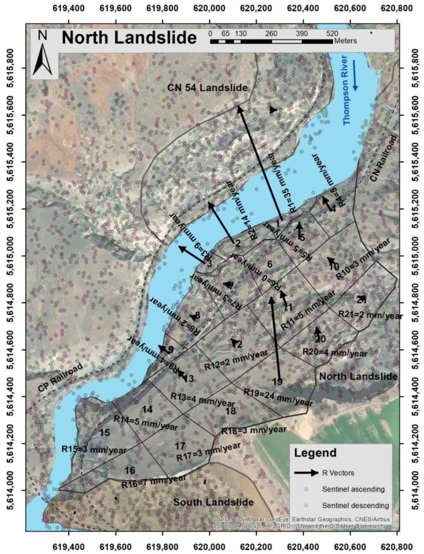
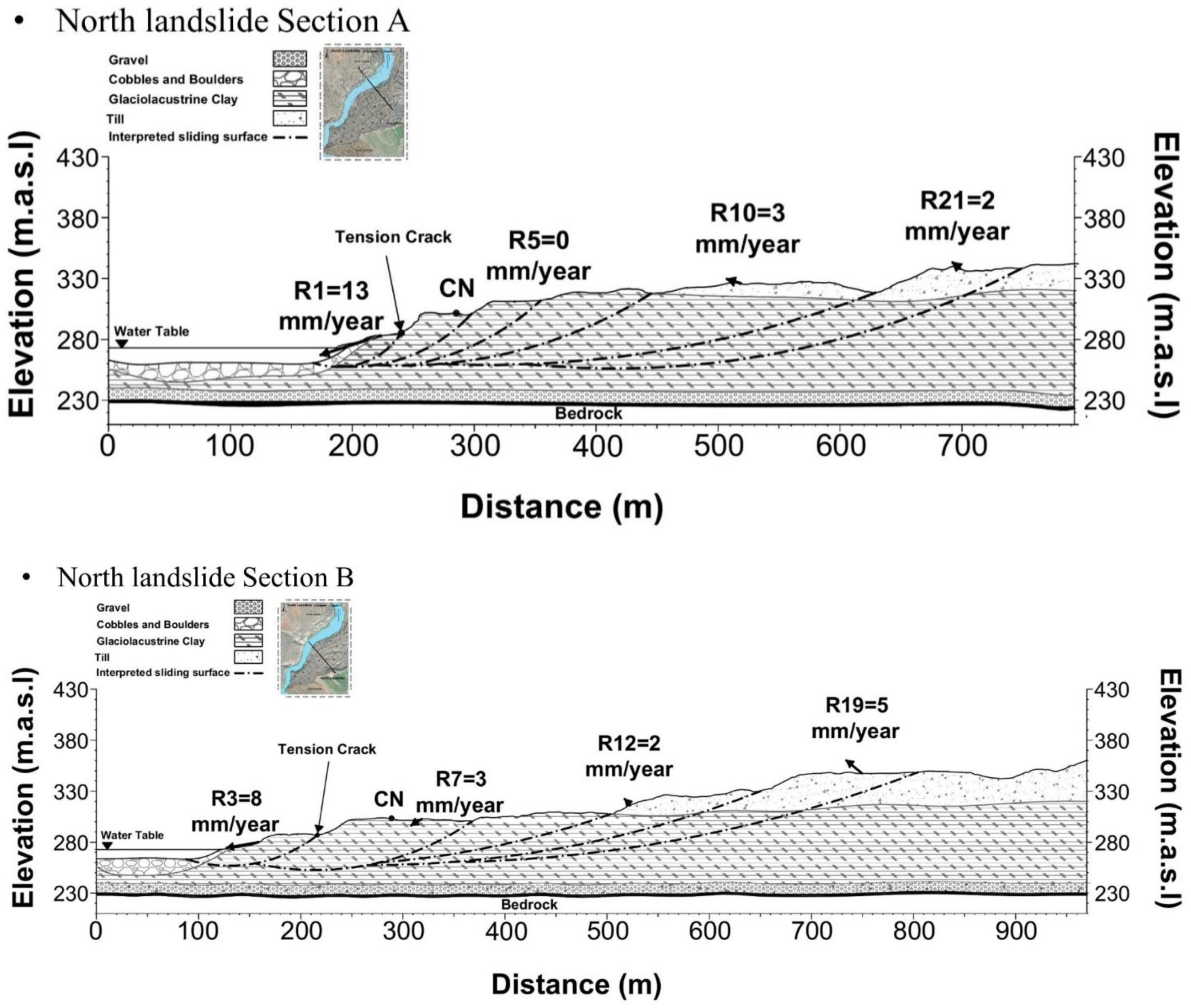
3.2. North Landslide

The recorded 2-year cumulative LOS displacements are presented in Figure 8. Ground movement in these 2 years is very limited in the North landslide (less than 10 mm/year) for most sectors except for sectors 2 and 3, and some parts of sector 1 for the descending orbit, which are located on the toe of the North landslide. Figure 9 shows the cumulative LOS displacements over these 2 years.

In all sectors except sector 3, LOS displacements are in the range of ±10 mm (ascending) and up to 25 mm at the end of the time period. The cumulative LOS displacements are ±10 mm (descending) for all sectors except sectors 1, 2, and 3. The maximum displacement occurred in sector 1 (approximately 50 mm in 2 years).

The horizontal components of R are shown in Figure 10. The maximum calculated horizontal component is 35 mm/year (sector 1). This magnitude is between 2 and 24 mm/year for other sectors, and higher activity is observed on the toe of the landslide (sectors 1, 2, and 3). Figure 11 shows the calculated R in selected sections on the North landslide. The vertical component of ground movement is negligible for most sectors except sectors 1 and 2 on the landslide’s toe. Some vertical components show upward movement, likely due to displacement magnitudes within the limits of detection of the technology and method adopted in this paper, and it is clear that most of the landslide shows minimum to no activity with the exception of some locations at the toe.

Table 4. Summary of calculated R magnitude and geometry for the North landslide.

Area	Recorded Date	Total Magnitude (mm/year)	Horizontal Magnitude (mm/year)	X Direction Component (mm/year)	Y Direction Component (mm/year)	Z Direction Component (mm/year)	Azimuth Angle (degree)	Angle with Horizontal Plane (degree)
R1	May 2015 to May 2017	35	35	−12	32	−4	339	7
R2	May 2015 to May 2017	16	14	−8	12	−8	328	28
R3	May 2015 to May 2017	9	9	−8	5	1	303	8
R4	May 2015 to May 2017	5	5	−2	4	0	330	3
R5	May 2015 to May 2017	5	5	0	5	0	0	3
R6	May 2015 to May 2017	0	0	0	0	0	−	−
R7	May 2015 to May 2017	3	3	−3	1	−2	282	30
R8	May 2015 to May 2017	2	2	−2	1	1	295	18
R9	May 2015 to May 2017	4	4	−3	1	−2	282	3
R10	May 2015 to May 2017	4	3	−3	2	0	306	3
R11	May 2015 to May 2017	5	5	−2	4	2	339	18
R12	May 2015 to May 2017	3	2	−1	2	2	318	39
R13	May 2015 to May 2017	4	4	−2	3	0	322	2
R14	May 2015 to May 2017	5	5	−3	5	0	327	1
R15	May 2015 to May 2017	3	3	−2	2	0	307	4
R16	May 2015 to May 2017	7	7	−2	7	0	344	3
R17	May 2015 to May 2017	3	3	−2	2	0	311	4
R18	May 2015 to May 2017	3	3	−2	2	1	318	12
R19	May 2015 to May 2017	24	24	−2	23	4	354	9
R20	May 2015 to May 2017	4	4	−1	3	2	346	29
R21	May 2015 to May 2017	2	2	−2	1	1	292	38

summarizes the calculated components of R for all sectors of the North landslide.

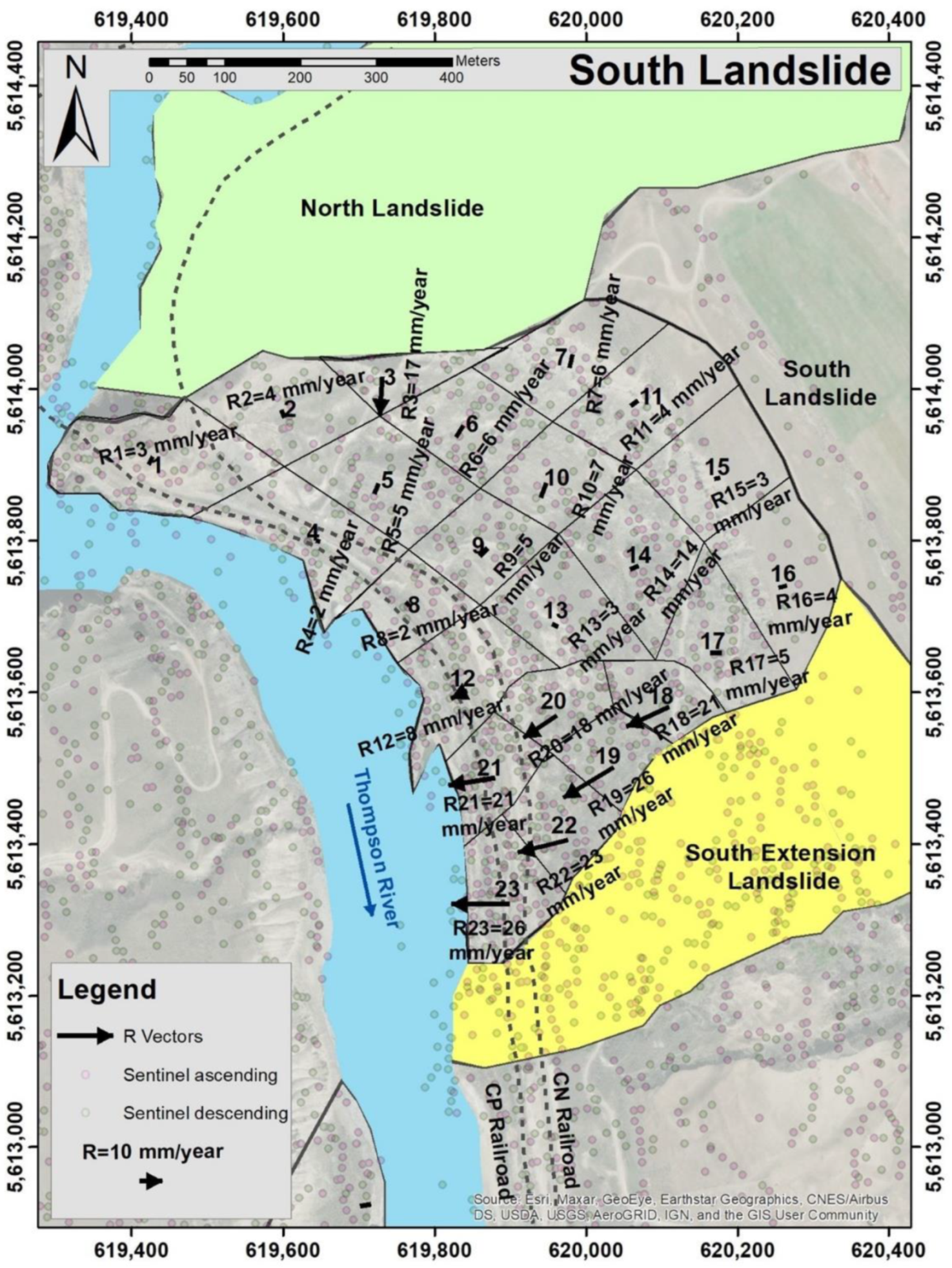
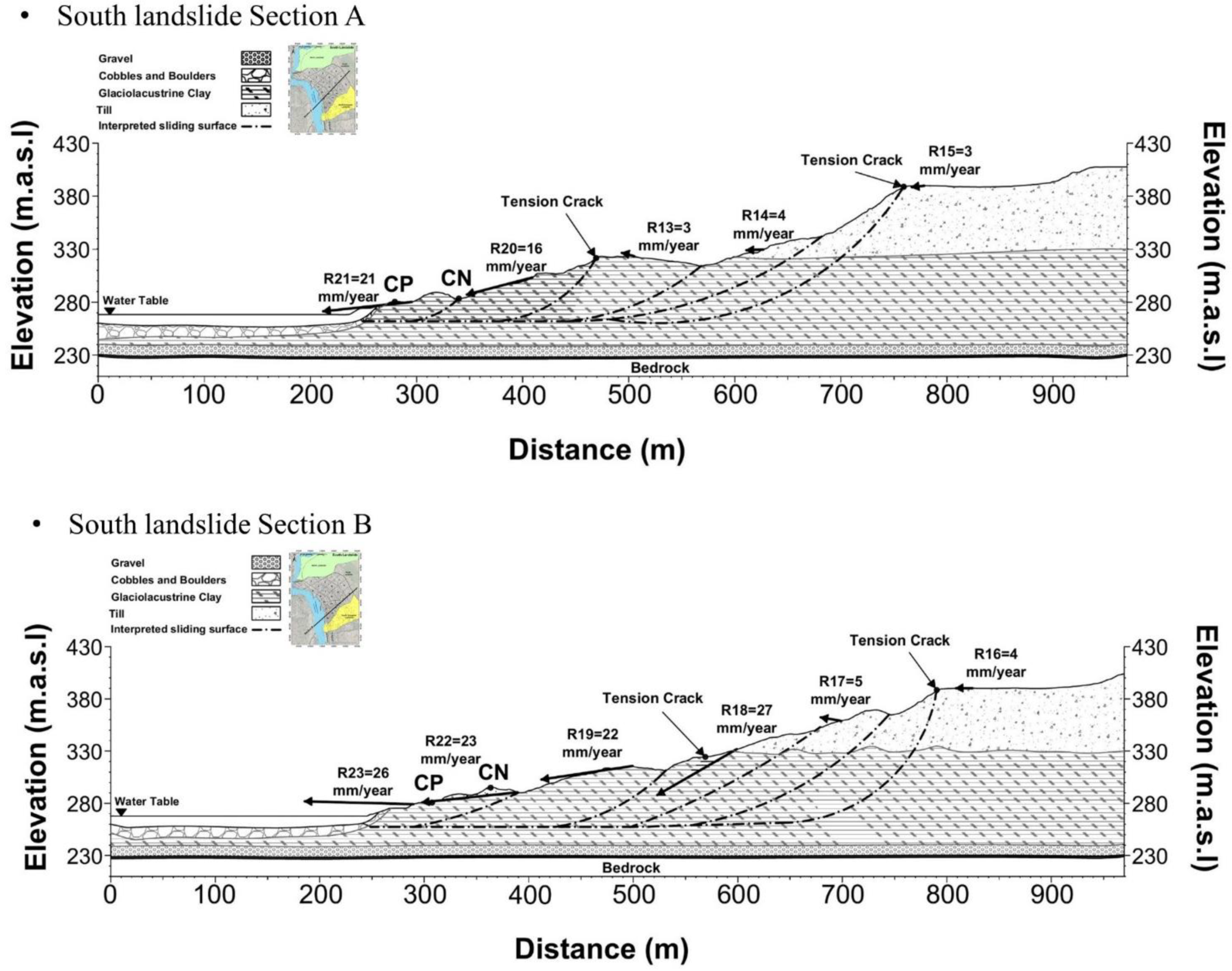
3.3. South Landslide

The cumulative 2-year LOS displacement is shown in Figure 12. The LOS displacements for different sectors are low on this landslide except for sectors 18 to 23, which are located on the landslide’s toe and upwards, in the south portion of the landslide. Figure 13 shows the cumulative LOS displacements of each sector. The 2-year displacements are in the range of ±10 mm for almost all sectors except sectors 18 to 23. The maximum displacements are over 40 mm in sector 23 (ascending) and approximately −50 mm in sector 18 (descending). Movements appear to accelerate in late summer and decelerate in spring, corresponding to river fluctuation (acceleration corresponds to river lows and a drawdown effect as identified for the Ripley Landslide in Hendry et al., 2015 [17]).

Figure 14 shows the results of calculated R. This figure shows the horizontal component, which varies between 2 and 26 mm/year for different sectors of the landslide. The landslide appears inactive in all sectors except in the south region. Figure 15 shows calculated R in selected cross-sections. The vertical component of movement is larger in sector 18 further upslope than river elevation in comparison to other sectors at the toe.

Table 5. Summary of calculated R magnitude and geometry for the South landslide.

Area	Recorded Date	Total Magnitude (mm/year)	Horizontal Magnitude (mm/year)	X Direction Component (mm/year)	Y Direction Component (mm/year)	Z Direction Component (mm/year)	Azimuth Angle (degree)	Angle with Horizontal Plane (degree)
R1	May 2015 to May 2017	3	3	−1	−3	0	207	1
R2	May 2015 to May 2017	4	4	−2	4	0	157	4
R3	May 2015 to May 2017	17	17	−1	−17	−3	184	10
R4	May 2015 to May 2017	2	2	−1	−2	0	196	6
R5	May 2015 to May 2017	5	5	−2	−5	1	200	7
R6	May 2015 to May 2017	6	6	−3	−5	1	211	8
R7	May 2015 to May 2017	6	6	−1	−6	−3	192	26
R8	May 2015 to May 2017	3	2	−1	−2	3	222	49
R9	May 2015 to May 2017	5	5	−3	−5	−1	210	11
R10	May 2015 to May 2017	7	7	−2	−7	1	199	8
R11	May 2015 to May 2017	4	4	−3	−2	0	232	0
R12	May 2015 to May 2017	8	8	−7	−4	0	243	2
R13	May 2015 to May 2017	3	3	−3	1	1	295	13
R14	May 2015 to May 2017	4	4	−4	−2	0	247	2
R15	May 2015 to May 2017	3	3	−3	−1	0	258	7
R16	May 2015 to May 2017	4	4	−4	−1	1	270	11
R17	May 2015 to May 2017	5	5	−5	0	1	270	11
R18	May 2015 to May 2017	24	21	−19	−9	−11	245	27
R19	May 2015 to May 2017	26	26	−22	−13	−1	239	3
R20	May 2015 to May 2017	19	18	−15	−10	−4	236	12
R21	May 2015 to May 2017	21	21	−21	−3	−2	261	10
R22	May 2015 to May 2017	23	23	−22	−6	−4	256	10
R23	May 2015 to May 2017	26	26	−26	0	1	270	1

shows the different components of R and their geometric characteristics.

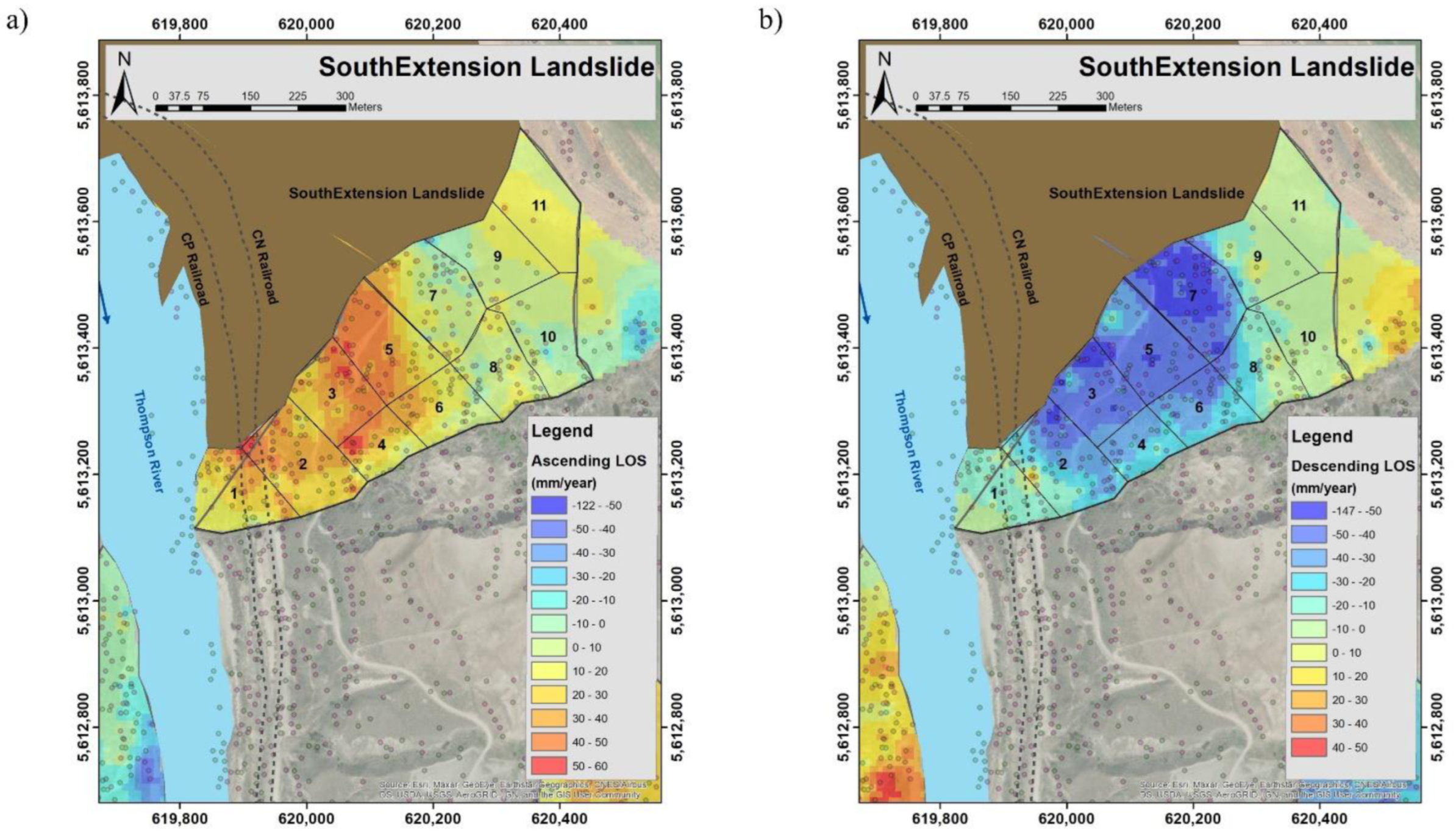
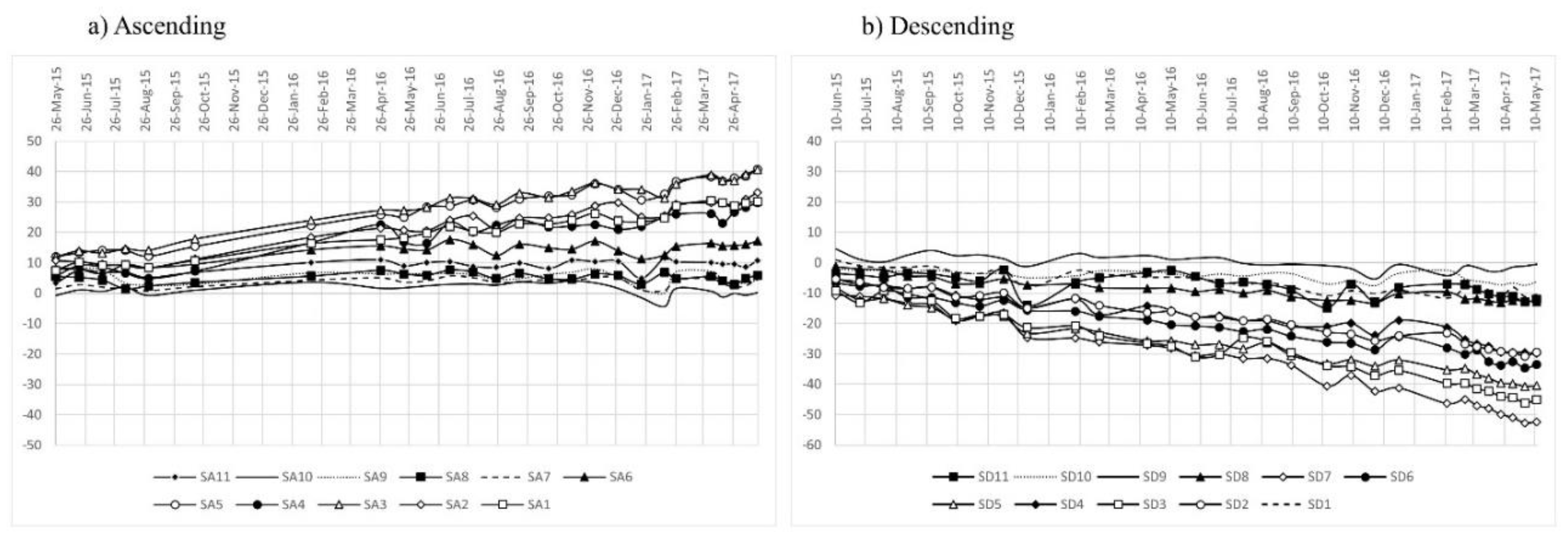
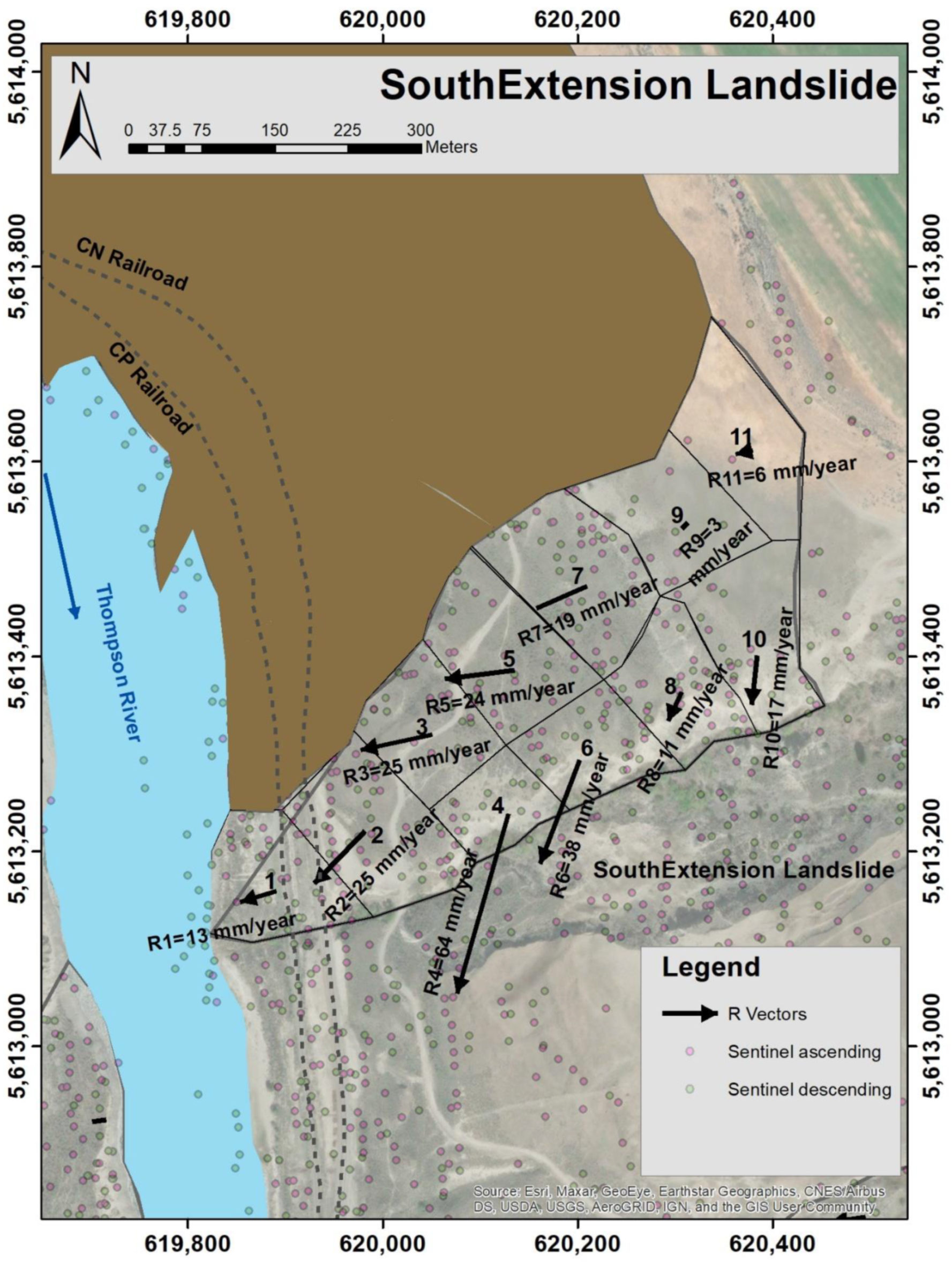
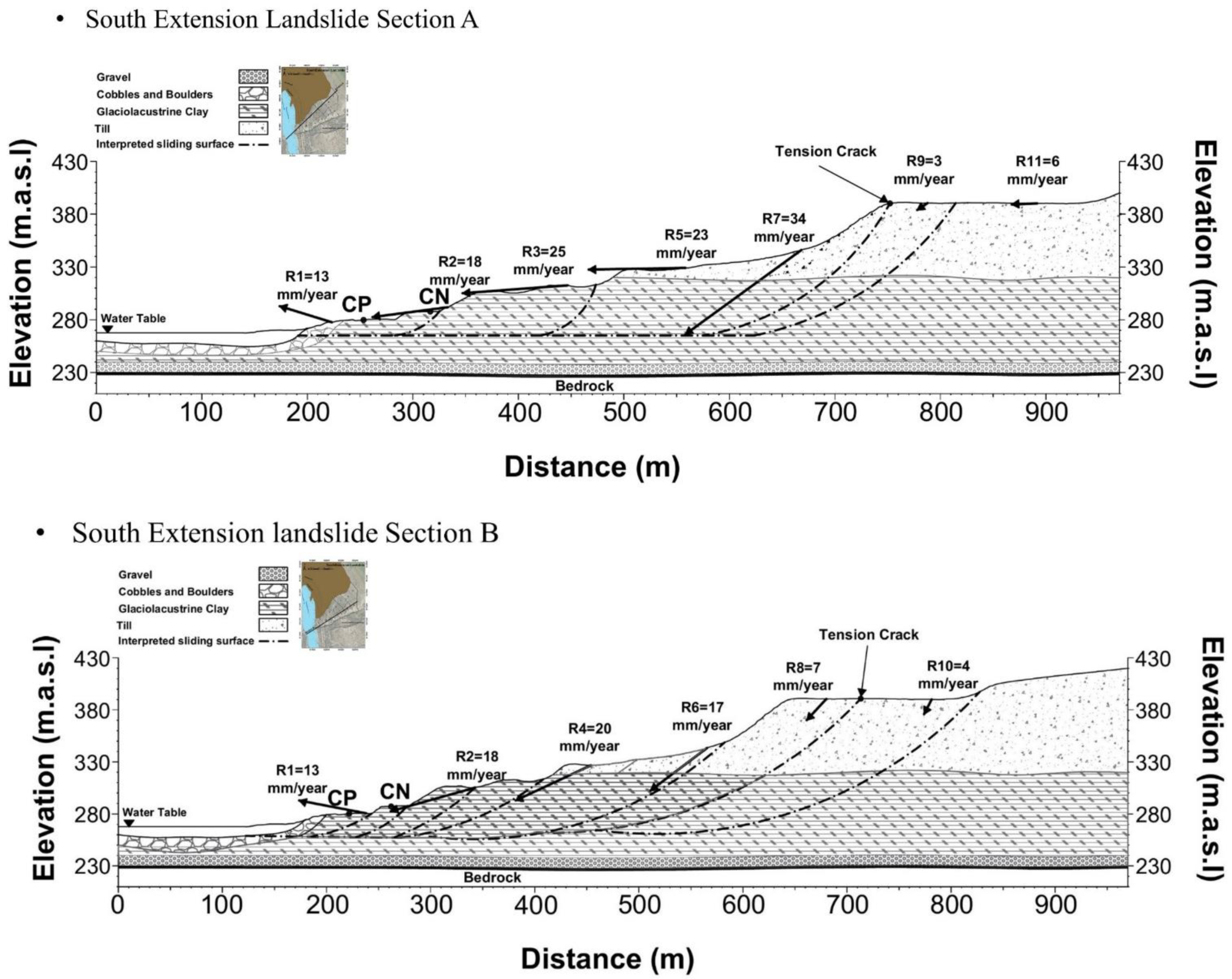
3.4. South Extension Landslide

The cumulative LOS displacement for the South Extension landslide is shown in Figure 16. The South Extension landslide is located immediately south of the South landslide, therefore earning its name. The landslide seems more active in sectors 1 to 8 (at and near the toe) while it seems the other sectors are less active. Figure 17 shows the time series of cumulative LOS displacement. It is shown that the cumulative LOS displacement does not exceed 10 mm for sectors 7, 8, 9, 10, and 11 for the ascending orbit and −10 for sectors 1, 9, 8, 10, and 11 for the descending orbit. The maximum cumulative 2-year LOS displacements are over 40 mm (ascending) and −50 mm (descending). There are also some observed periods of acceleration for sectors 2 to 7. Movements appear to accelerate in late summer and decelerate in spring, corresponding to river fluctuation (acceleration corresponds to river lows and a drawdown effect as identified for the Ripley Landslide in Hendry et al., 2015 [10].

The horizontal components of calculated R for the South Extension landslide are shown in Figure 18. The magnitude of the horizontal component of R varies between 3 mm/year for sector 9 in the Northeast area of the landslide, and 64 mm/year for sector 4 on the south boundary of the landslide.

The vertical components of R on the South Extension landslide are shown in Figure 19 for selected sectors of the landslide and selected cross sections. Movement is predominantly horizontal near the toe of the landslide and some sectors upslope and near the back scarp show increased vertical components of movement. Movement is negligible behind the back scarp, suggesting no landslide retrogression beyond that elevation.

Table 6. Summary of calculated R magnitude and geometry for the South Extension landslide.

Area	Recorded Date	Total Magnitude (mm/year)	Horizontal Magnitude (mm/year)	X Direction Component (mm/year)	Y Direction Component (mm/year)	Z Direction Component (mm/year)	Azimuth Angle (degree)	Angle with Horizontal Plane (degree)
R1	May 2015 to May 2017	14	13	−13	−4	4	253	16
R2	May 2015 to May 2017	25	25	−18	−18	−2	224	5
R3	May 2015 to May 2017	25	25	−25	−5	−2	258	4
R4	May 2015 to May 2017	65	64	−18	−62	−8	196	7
R5	May 2015 to May 2017	24	24	−23	−3	0	263	1
R6	May 2015 to May 2017	39	38	−14	−35	−10	201	15
R7	May 2015 to May 2017	23	19	−18	−8	−13	246	34
R8	May 2015 to May 2017	12	11	−5	−10	−5	205	24
R9	May 2015 to May 2017	4	3	−2	−2	−2	225	26
R10	May 2015 to May 2017	18	17	−2	−17	−4	186	12
R11	May 2015 to May 2017	6	6	−6	−1	0	257	2

presents the components of the calculated R for all sectors of the South Extension landslide, including the component magnitudes and the geometry of R.

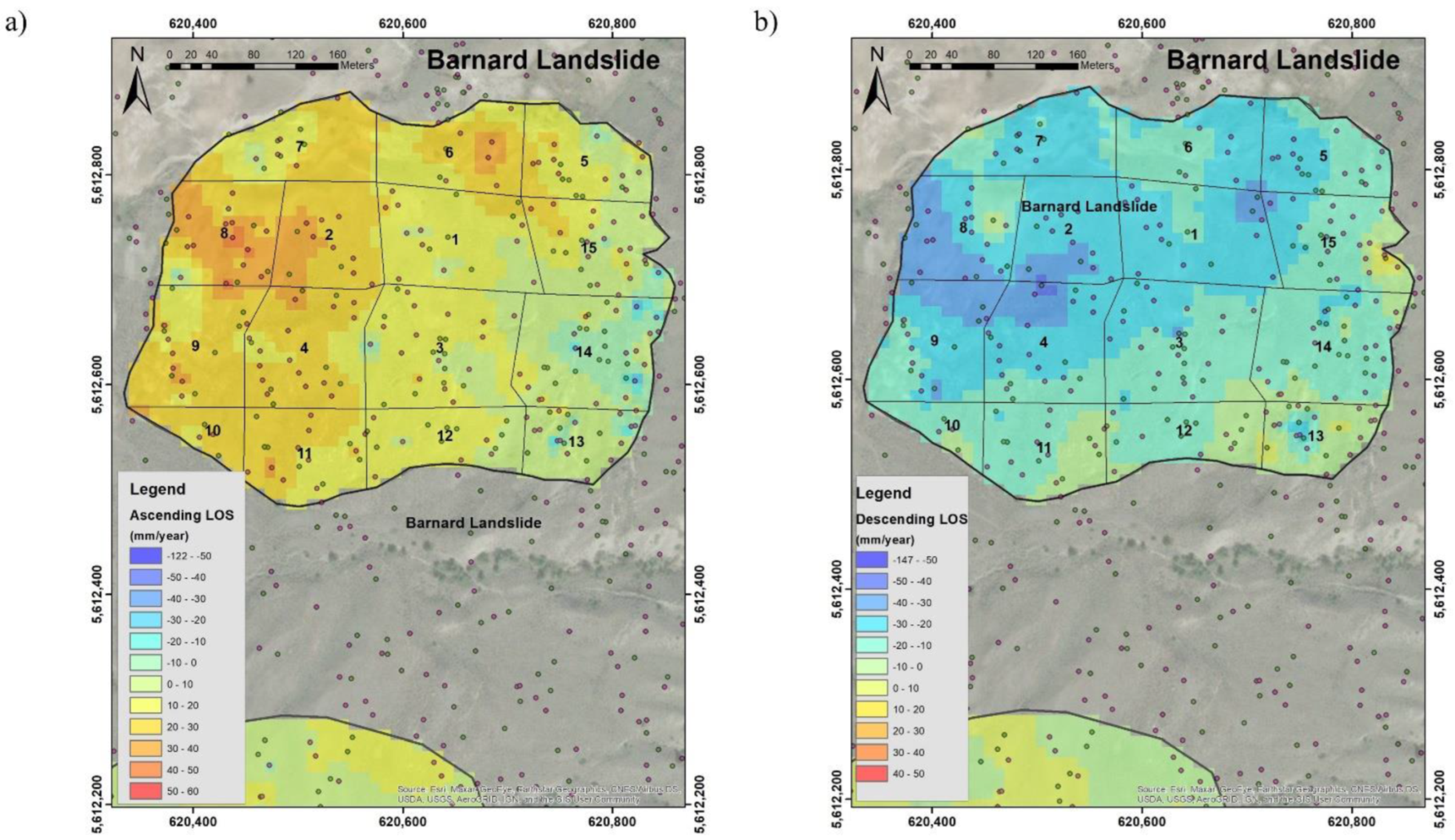
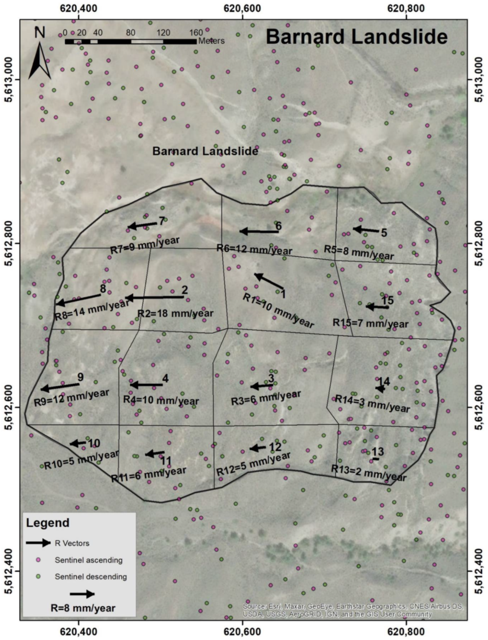
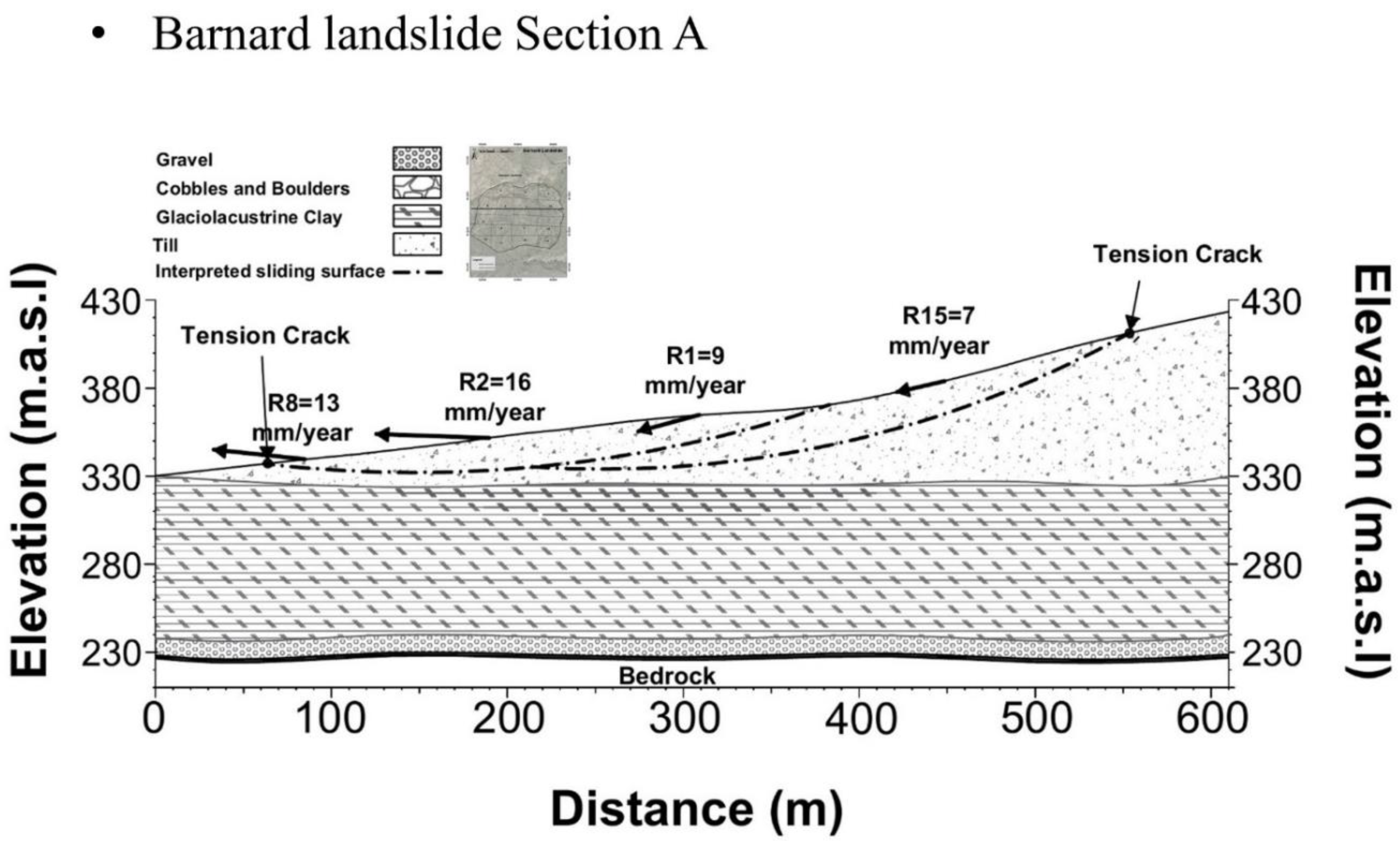
3.5. Barnard Landslide

The Barnard landslide cumulative 2-year LOS displacements are shown in Figure 20. The magnitudes of LOS displacements are larger at and near the toe of the landslide. The time series of the 2-year cumulative LOS displacements are shown in Figure 21 for all sectors of the Barnard landslide. The magnitude of the cumulative LOS displacement in these 2 years ranges between +30 and −30 for both orbits.

The calculated horizontal components of R on the Barnard landslide are shown in Figure 22. The magnitude of the horizontal displacements is between 2 and 18 mm/year, with the maximum horizontal displacement at sector 2, in the center of the landslide. The vertical components of R are shown in Figure 23. Ground displacements are near horizontal at or near the toe of the landslide, while the vertical component of ground displacements increases in sectors to the east of the landslide. The higher vertical components of R near the crest, transitioning towards near horizontal movement and showing some upward component near the toe, suggest a predominantly circular kinematic motion.

Table 7. Summary of calculated R components magnitude and vector geometry at the Barnard landslide.

Area	Recorded Date	Total Magnitude (mm/year)	Horizontal Magnitude (mm/year)	X Direction Component (mm/year)	Y Direction Component (mm/year)	Z Direction Component (mm/year)	Azimuth Angle (degree)	Angle with Horizontal Plane (degree)
R1	May 2015 to May 2017	10	10	−9	4	−3	297	15
R2	May 2015 to May 2017	18	18	−16	8	1	297	2
R3	May 2015 to May 2017	7	6	−6	0	−3	266	29
R4	May 2015 to May 2017	10	10	−10	0	−1	270	3
R5	May 2015 to May 2017	8	8	−8	1	−2	276	10
R6	May 2015 to May 2017	12	12	−12	0	1	271	6
R7	May 2015 to May 2017	9	9	−9	−1	−1	262	4
R8	May 2015 to May 2017	14	14	−13	−3	1	258	6
R9	May 2015 to May 2017	12	12	−12	−2	−3	262	14
R10	May 2015 to May 2017	7	5	−5	−1	4	264	37
R11	May 2015 to May 2017	6	6	−6	−1	0	262	1
R12	May 2015 to May 2017	5	5	−5	−1	0	263	0
R13	May 2015 to May 2017	3	2	−2	0	−2	275	44
R14	May 2015 to May 2017	5	3	−3	0	−4	278	48
R15	May 2015 to May 2017	7	7	−7	0	−2	273	13

summarizes the components of calculated R and the geometry of these vectors.

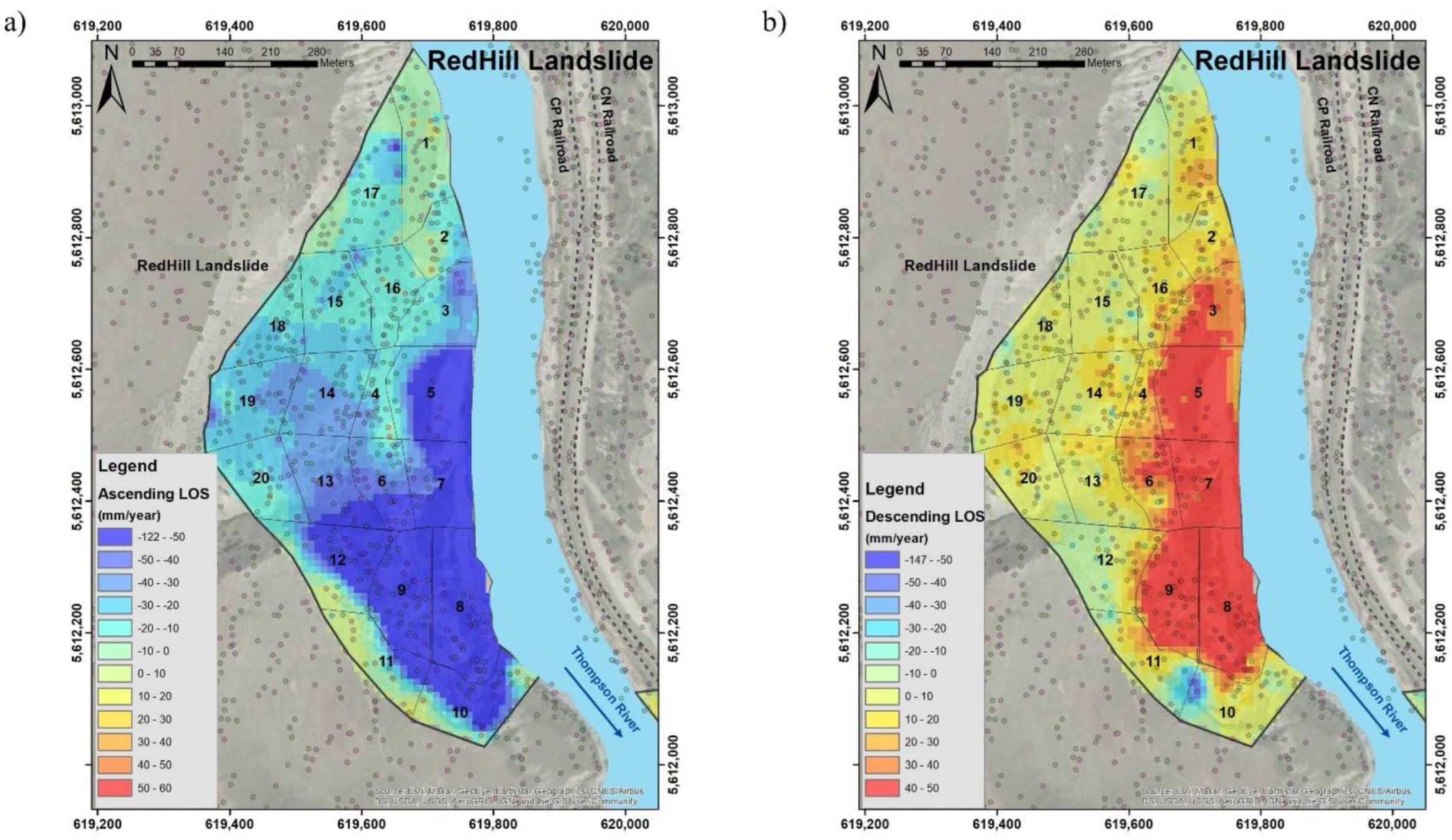
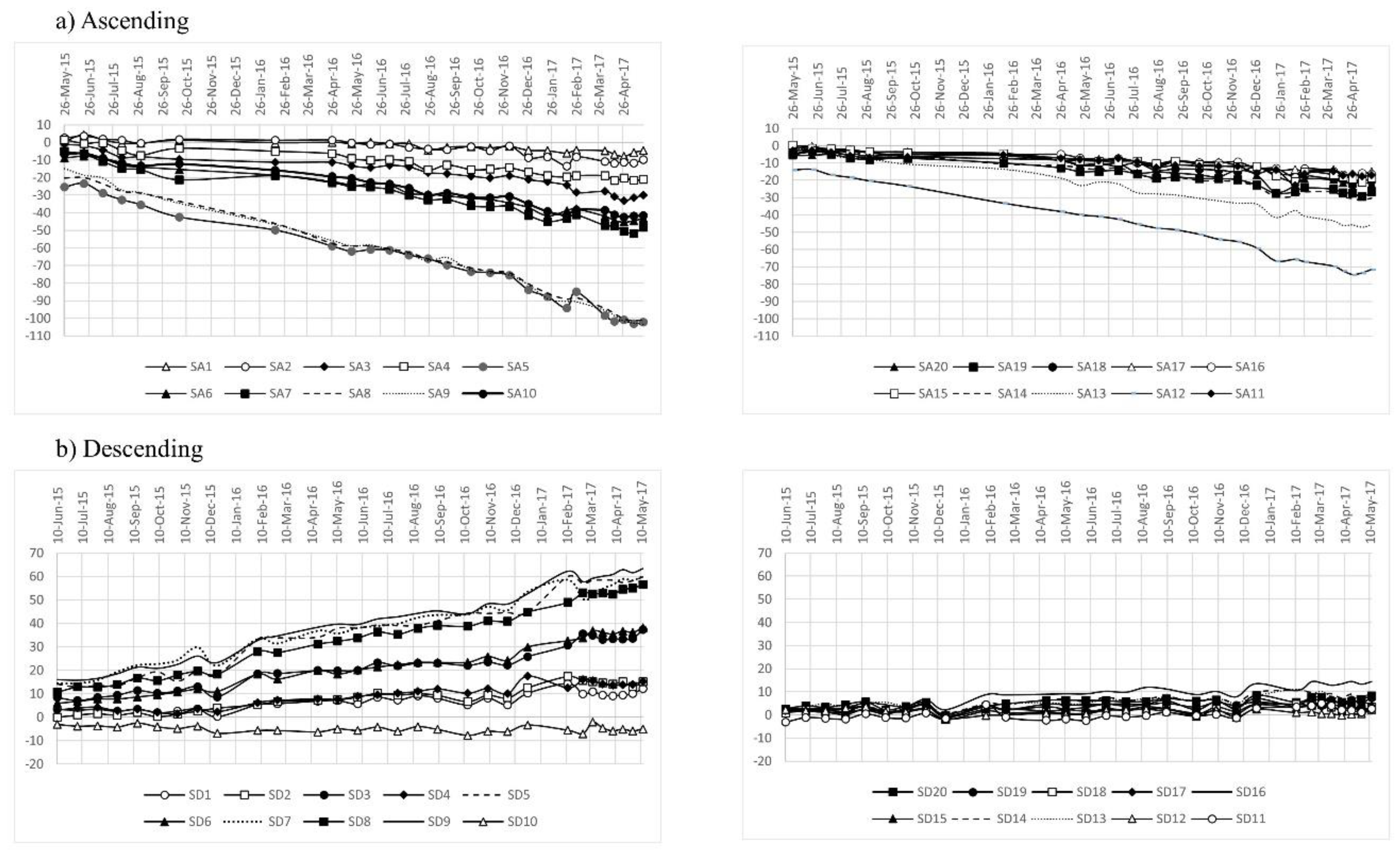
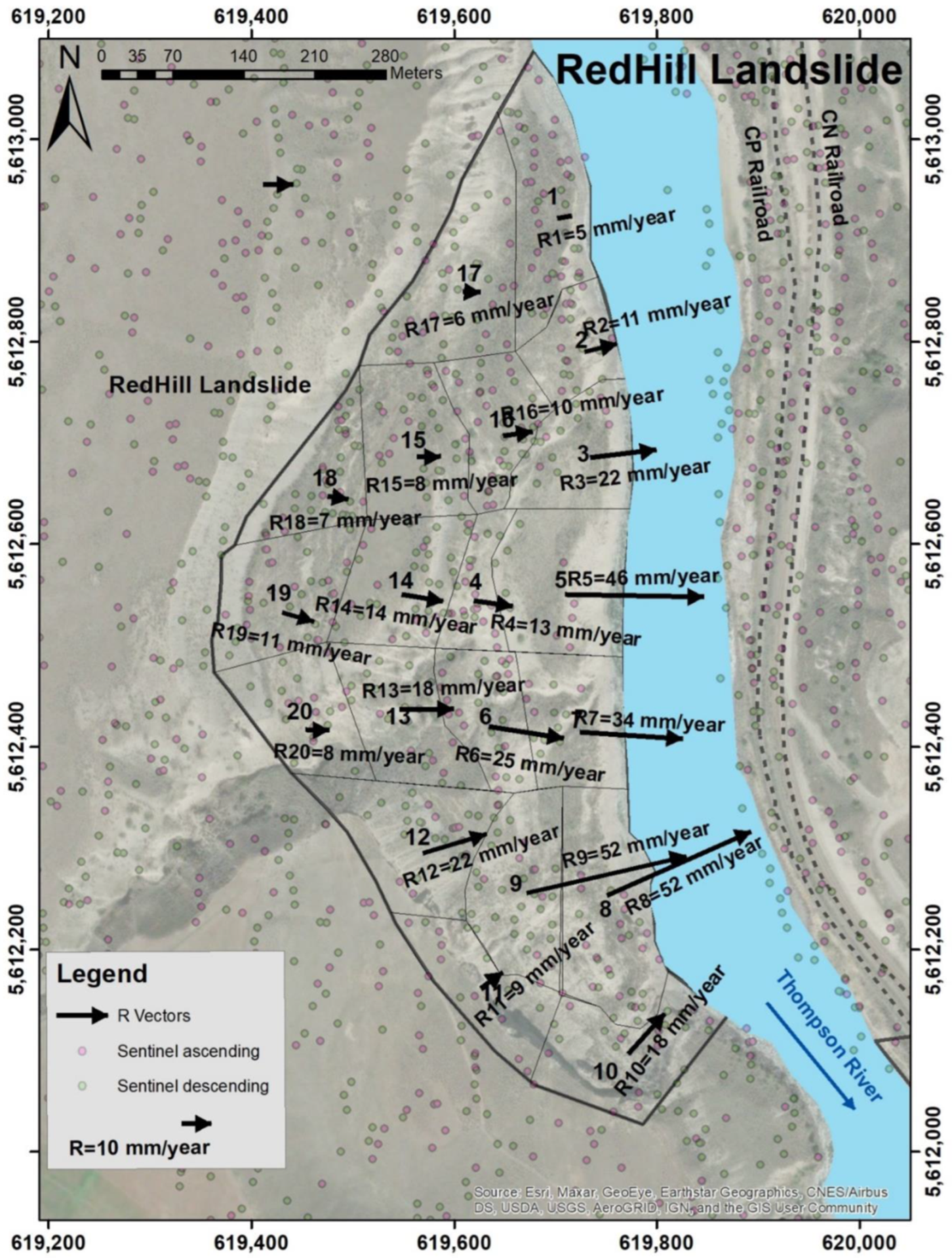
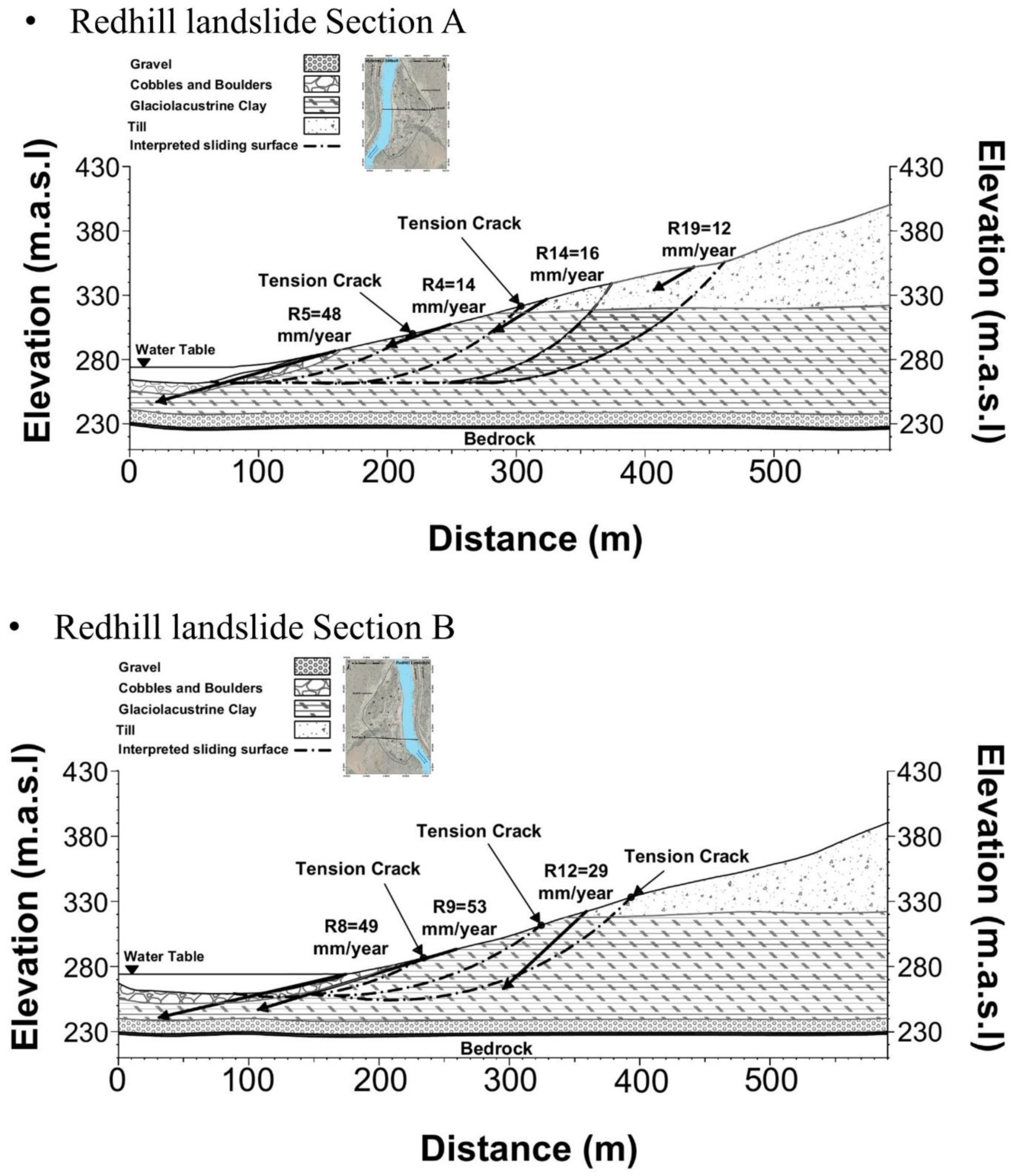
3.6. Redhill Landslide

The cumulative 2-year LOS displacements at the Redhill landslide are shown in Figure 24. The toe of the Redhill landslide appears to be the most active area of the landslide. The 2-year time series of cumulative LOS displacements are shown in Figure 25. The toe of this landslide is the most active of all landslides in this paper. The cumulative LOS displacements exceed −100 mm (ascending) and 60 mm (descending). Sectors at the backscarp (11–20) have cumulative LOS displacements between −30 mm and +20 mm (considering both orbits).

Figure 26 shows the horizontal component of calculated R for the Redhill landslide. Sectors 8 and 9 show the most activity, with displacements of up to 52 mm/year. The magnitude of the horizontal component for other sectors of the landslide varies between 5 and 46 mm/year.

The vertical components of R for selected sectors of the landslide are shown in Figure 27. This figure shows that ground displacements have a significant vertical component regardless of the distance from the toe or the back scarp, transitioning towards fewer vertical components near the toe. This would indicate that the toe of the landslide is likely well into the riverbed that could not be captured by the Satellite InSAR data available.

Table 8. Summary of calculated R magnitude, components, and geometry on the Redhill landslide.

Area	Recorded Date	Total Magnitude (mm/year)	Horizontal Magnitude (mm/year)	X Direction Component (mm/year)	Y Direction Component (mm/year)	Z Direction Component (mm/year)	Azimuth Angle (degree)	Angle with Horizontal Plane (degree)
R1	May 2015 to May 2017	6	5	5	1	1	81	11
R2	May 2015 to May 2017	11	11	10	3	1	75	4
R3	May 2015 to May 2017	22	22	22	3	−1	83	2
R4	May 2015 to May 2017	14	13	13	−2	−4	98	18
R5	May 2015 to May 2017	48	46	46	−1	−13	91	16
R6	May 2015 to May 2017	25	25	25	0	−2	89	4
R7	May 2015 to May 2017	34	34	34	−2	−1	94	2
R8	May 2015 to May 2017	53	52	48	21	−11	66	12
R9	May 2015 to May 2017	54	52	51	12	−15	77	16
R10	May 2015 to May 2017	21	18	12	13	−11	42	32
R11	May 2015 to May 2017	9	9	7	5	−2	54	14
R12	May 2015 to May 2017	29	22	21	6	−19	73	41
R13	May 2015 to May 2017	23	18	18	0	−14	89	37
R14	May 2015 to May 2017	16	14	13	−2	−8	99	31
R15	May 2015 to May 2017	10	8	8	0	−6	89	37
R16	May 2015 to May 2017	11	10	10	1	−2	82	9
R17	May 2015 to May 2017	8	6	6	0	−5	93	40
R18	May 2015 to May 2017	8	7	7	−1	−5	99	36
R19	May 2015 to May 2017	13	11	11	−3	−6	106	29
R20	May 2015 to May 2017	9	8	8	0	−4	91	64

summarizes the components and geometry of calculated R. The total magnitude of R is between 6 mm and 54 mm.

4. Summary and Discussion

Although the density of gathered data is different for each landslide in the research area, Figure 3 shows the data-density-guided selection of landslide sectors to balance information adequacy and availability for kinematic analysis. To calculate the R vectors, we require data from both orbits within each sector, where sectors are defined such that the data density is enough for all defined sectors of each landslide. The exception in this research was sector 2 of the Goddard landslide, with a lack of descending orbit data.

Figure 4 and Figure 8 show low activity recorded by Sentinel 1 (LOS) for most parts of the Goddard and North landslides, with increased activity on sectors 1, 2, and 3 on the toe of the North landslide. Figure 12 shows low activity for the South landslide, except for sectors 18 to 23. The South extension landslide is more active according to Figure 16 on those sectors that have a common boundary with the South landslide, suggesting the south extension is likely a lateral retrogression of the South Landslide. Figure 20 illustrates two different trends of the activity measured on the west and east sectors of the Barnard landslide. However, this landslide shows low activity generally in all its sectors, and trends are likely masked by the limits of detection of the technology and assumptions in this work, combined. The activity of the Redhill landslide is relatively high, especially at its toe near the Thompson River in sectors 3 to 12, from both satellite orientations, as it is shown in Figure 24.

Despite the absence of a clear seasonal displacement trend in most landslide displacement data, this was likely due to the low cumulative LOS and measurement precision of the data (Figure 5, Figure 9, Figure 13, Figure 17, Figure 21 and Figure 25), precluding definitive interpretation of seasonal trends; movements appear to accelerate in late summer and decelerate in spring, corresponding to river fluctuation (acceleration corresponds to river lows and a drawdown effect as identified for the Ripley Landslide in Hendry et al., (2015) and Huntley (2021)) [16,17].

The horizontal component of R vectors for all sectors of the research area does not exceed 64 mm/year, which means all landslides in this area are classified as very slow-moving landslides based on velocity classification by Curden and Vernes (1996) [50,51]. The horizontal component of calculated ground movement for the Goddard landslide is between 2 and 29 mm/year (Figure 6) with the maximum movement calculated for sector 7. Figure 10 shows the magnitude of horizontal movement between 2 and 35 mm/year in the research timeline for the North landslide with the maximum movement in sector 1 on the landslide’s toe. This is consistent with previous findings [16]. Figure 14 and Figure 18 show the horizontal component of R vectors varies between 2 and 26 mm/year for South landslide and 3 to 64 mm/year for the South extension landslide as well. The more active parts of the South landslide are located near the boundary with the South Extension landslide, suggesting this extension is likely a lateral retrogression of the South landslide. The maximum displacement is observed for sector 4 of the South extension landslide and the direction of R vectors in the horizontal plane are different in the north and south parts of this landslide due to their different aspects. Air imagery inspection suggests that this change in displacement attitude is likely due to the presence of a gully at the south boundary of the South Extension landslide, allowing for the kinematics of the landslide to develop a southward trend of motion; however, this aspect is a matter of further investigation as the assumptions of the horizontal direction of movement directly define this directionality solely on a topographical basis. The reported magnitudes for these areas are consistent with previous findings [16].

Figure 22 shows the horizontal movements of the Barnard landslide between 2 and 18 mm/year, with the more active areas concentrated on the central sectors of the landslide and extending to the west, closer to the river. Figure 26 shows horizontal movement at the Red Hill landslide of between 5 and 52 mm/year, with the highest activity in sectors 8 and 9 at the toe of the landslide. The magnitude and activity are also consistent with previous studies [16].

Generally, the vertical component of the terrain movement changes based on both the distance from the river and the magnitude of movements for each specific sector of each landslide. It is observed in Figure 7 that the Goddard landslide moves more vertically on the toe of the landslide on sectors 1 and 3, and the back scarp for sectors 10 and 11 despite their lower movement. The movement is more horizontal in other sectors (15, 16, and 17). Figure 11 shows horizontal movement on the North landslide for almost all sectors except those at the toe, which move with larger vertical components. Vertical components of R vectors on the South landslide in Figure 15 also show small horizontal movement at the back scarp with more pronounced vertical components when compared to the toe of the landslide. Figure 19 also shows that for the South Extension landslide, the vertical components are relatively negligible for sectors at the toe in comparison to sectors closer to the back scarp. These results are consistent with compound kinematics of landslides, commonly defined by the presence of sub-horizontal weak layers that act as base sliding surfaces. Previous research had identified the presence of silt and clay layers with sub-horizontal bedding, which would be responsible for the landslide activity in this valley [7,19,42], and the kinematics observed through the results of this study support the hypothesis of compound mechanisms. This landslide mechanism based on the recent results shows this compound kinematic with soil masses moving on sub-horizontal basal sliding surfaces and being pushed by upslope driving wedges on near-planar to semi-circular sliding surfaces (e.g., the South landslide and the toe of the South Extension landslide).

Figure 26 illustrates almost horizontal movement for sectors of the Barnard landslide that are closer to the river on the west part of this landslide, while the vertical components are more notable for sectors on the east side of the Barnard landslide. The shear-interpreted surfaces using the reported R vectors in this figure suggest a rotational retrogressive landslide in this area with lower depth than other landslides in the research area due to the direction of movements of each sector and the locations of tension cracks observed in ground features.

The vertical component of R is consistent for most sectors within the Redhill in sections of Figure 27. The vertical and horizontal components of R in the section views suggest a retrogressive, rotational movement for the Redhill landslide, which is consistent with previous research [16].

5. Conclusions

Six landslides with the most significant impacts on the CN and CP railways were investigated in this research. These landslides are Goddard, North, South, South extension, Barnard, and Redhill, which are located from the north of the Thompson River valley to South, respectively. This valley is one of the most important transportation corridors in Canada and has experienced several landslides in its history. This paper presents a new understanding of landslides’ displacement and kinematics in this area using InSAR monitoring data gathered by the Sentinel 1 satellite from May 2015 to May 2017 from both ascending and descending orbits. To obtain more detailed displacements of each landslide, they are divided into different sectors to better understand their kinematics. A method is proposed where the horizontal component of movement is considered parallel to the slope azimuth in order to calculate an approximation of the three-dimensional ground displacement vector (R) using InSAR data from two orientations. The method was validated for a landslide in the study area against recorded GPS results on the Ripley landslide [47].

All landslides in this research are classified as very slow landslides according to the velocity classification by Curden and Vernes (1996) [42,50]. The total magnitude of movement in this area is reported between 2 and 64 mm/year for all landslides in this research.

Table 9. Summary of all monitored landslides along the Thompson River valley.

Landslide	Monitoring Timeline	Maximum Velocity (mm/year)	Minimum Velocity (mm/year)	Velocity Classification	Type of Landslide’s Kinematic
Goddard	May2015 to May 2017	2	29	Very Slow	Retrogressive rotational
North	May2015 to May 2017	2	35	Very Slow	Rotational on the toe
South	May2015 to May 2017	2	26	Very Slow	transitional
South Extension	May2015 to May 2017	3	64	Very Slow	Transitional on the toe + Retrogressive rotational
Barnard	May2015 to May 2017	2	18	Very Slow	Rotational retrogressive
Redhill	May2015 to May 2017	8	56	Very Slow	Retrogressive rotational

shows a summary of movements for each landslide studied. The maximum movement occurred in the South Extension landslide with a velocity of 64 mm/year while the Barnard is the slowest with a maximum velocity of 18 mm/year. The Redhill landslide is also one of the most active landslides in this research with a maximum velocity of 52 mm/year.

Ground displacements measured outside the known-active landslide areas were very low, suggesting minimum to no retrogression activity (except for the interpretation discussed for the South Extension landslide).

The approach presented for landslide investigation based on combining Satellite InSAR orientations, assumptions of landslide horizontal displacement direction based on topographic characteristics and averaging of space and time inconsistencies between different LOS orientation acquisition provides valuable additional insight into common interpretation of East–West and vertical components. The work in this paper illustrates how the added benefits of the approach include enhanced characterization of landslide kinematics and the state of activity. It is important to note that the assumption of landslide directionality needs to be evaluated on a case-by-case, as surface topographic characteristics could mislead the horizontal orientation of movement for complex mechanisms.

References

1. Charrière, M.; Humair, F.; Froese, C.; Jaboyedoff, M.; Pedrazzini, A.; Longchamp, C. From the source area to the deposit: Collapse, fragmentation, and propagation of the Frank Slide. GSA Bull. 2016, 128, 332–351. [Google Scholar] [CrossRef]
2. Cruden, D.M.; Martin, C.D. Before the Frank Slide. Can. Geotech. J. 2007, 44, 765–780. [Google Scholar] [CrossRef]
3. Mei, S.; Poncos, V.; Froese, C. Mapping millimetre-scale ground deformation over the underground coal mines in the Frank Slide area, Alberta, Canada, using spaceborne InSAR technology. Can. J. Remote Sens. 2008, 34, 113–134. [Google Scholar] [CrossRef]
4. Vallee, M. Falling in Place: Geoscience, Disaster, and Cultural Heritage at the Frank Slide, Canada’s Deadliest Rockslide. Space Cult. 2019, 22, 66–76. [Google Scholar] [CrossRef]
5. Choe, B.-H.; Blais-Stevens, A.; Samsonov, S.; Dudley, J. Sentinel-1 and RADARSAT Constellation Mission InSAR Assessment of Slope Movements in the Southern Interior of British Columbia, Canada. Remote Sens. 2021, 13, 3999. [Google Scholar] [CrossRef]
6. Huntley, D.; Bobrowsky, P.; Hendry, M.; Macciotta, R.; Elwood, D.; Sattler, K.; Best, M.; Chambers, J.; Meldrum, P. Application of multi-dimensional electrical resistivity tomography datasets to investigate a very slow-moving landslide near Ashcroft, British Columbia, Canada. Landslides 2019, 16, 1033–1042. [Google Scholar] [CrossRef]
7. Journault, J.; Macciotta, R.; Hendry, M.T.; Charbonneau, F.; Huntley, D.; Bobrowsky, P.T. Measuring displacements of the Thompson River valley landslides, south of Ashcroft, BC, Canada, using satellite InSAR. Landslides 2018, 15, 621–636. [Google Scholar] [CrossRef]
8. Macciotta, R.; Hendry, M.; Martin, C.D. Developing an early warning system for a very slow landslide based on displacement monitoring. Nat. Hazards 2016, 81, 887–907. [Google Scholar] [CrossRef]
9. Rodriguez, J.; Deane, E.; Hendry, M.; Macciotta, R.; Evans, T.; Gräpel, C.; Skirrow, R. Practical evaluation of single-frequency dGNSS for monitoring slow-moving landslides. Landslides 2021, 18, 3671–3684. [Google Scholar]
10. Macciotta, R.; Hendry, M. Remote Sensing Applications for Landslide Monitoring and Investigation in Western Canada. Remote Sens. 2021, 13, 366. [Google Scholar] [CrossRef]
11. Lan, H.; Zhao, X.; Macciotta, R.; Peng, J.; Li, L.; Wu, Y.; Zhu, Y.; Liu, X.; Zhang, N.; Liu, S.; et al. The cyclic expansion and contraction characteristics of a loess slope and implications for slope stability. Sci. Rep. 2021, 11, 2250. [Google Scholar] [CrossRef] [PubMed]
12. Woods, A.; Macciotta, R.; Hendry, M.; Stewart, T.; Marsh, J. Updated understanding of the deformation characteristics of the Checkerboard Creek rock slope through GB-InSAR monitoring. Eng. Geol. 2020, 281, 105974. [Google Scholar] [CrossRef]
13. Macciotta, R.; Gräpel, C.; Skirrow, R. Fragmented Rockfall Volume Distribution from Photogrammetry-Based Structural Mapping and Discrete Fracture Networks. Appl. Sci. 2020, 10, 6977. [Google Scholar] [CrossRef]
14. Deane, E.; Macciotta, R.; Hendry, M.; Gräpel, C.; Skirrow, R. Leveraging historical aerial photographs and digital photogrammetry techniques for landslide investigation—A practical perspective. Landslides 2020, 17, 1989–1996. [Google Scholar] [CrossRef]
15. Huntley, D.; Rotheram-Clarke, D.; Cocking, R.; Joseph, J.; Bobrowsky, P. Understanding plateau and prairie landslides: Annual report on landslide research in the Thompson River valley, British Columbia, and the Assiniboine River valley, Manitoba-Saskatchewan 2020–2021. Geol. Surv. Can. 2021, 8838, 3–73. [Google Scholar]
16. Huntley, D.; Rotheram-Clarke, D.; Pon, A.; Tomaszewicz, A.; Leighton, J.; Cocking, R.; Joseph, J. Benchmarked RADARSAT-2, SENTINEL-1 and RADARSAT Constellation Mission Change-Detection Monitoring at North Slide, Thompson River Valley, British Columbia: Ensuring a Landslide-Resilient National Railway Network. Can. J. Remote Sens. 2021, 47, 635–656. [Google Scholar] [CrossRef]
17. Hendry, M.T.; Macciotta, R.; Martin, C.D.; Reich, B. Effect of Thompson River elevation on velocity and instability of Ripley Slide. Can. Geotech. J. 2015, 52, 257–267. [Google Scholar] [CrossRef]
18. Huntley, D.; Bobrowsky, P.; Hendry, M.; Macciotta, R.; Best, M. Multi-technique Geophysical Investigation of a Very Slow-moving Landslide near Ashcroft, British Columbia, Canada. J. Environ. Eng. Geophys. 2019, 24, 87–110. [Google Scholar] [CrossRef]
19. Eshraghian, A.; Martin, D.; Cruden, D. Complex Earth Slides in the Thompson River Valley, Ashcroft, British Columbia. Environ. Eng. 2007, 13, 161–181. [Google Scholar] [CrossRef]
20. Huntley, D.; Holmes, J.; Bobrowsky, P.; Chambers, J.; Meldrum, P.; Wilkinson, P.; Donohue, S.; Elwood, D.; Sattler, K.; Hendry, M.; et al. Hydrogeological and geophysical properties of the very slow-moving Ripley Landslide, Thompson River valley, British Columbia. Can. J. Earth Sci. 2020, 57, 1371–1391. [Google Scholar] [CrossRef]
21. Sattler, K.; Elwood, D.; Hendry, M.T.; Huntley, D.; Holmes, J.; Wilkinson, P.B.; Chambers, J.; Donohue, S.; Meldrum, P.I.; Macciotta, R.; et al. Quantifying the contribution of matric suction on changes in stability and displacement rate of a translational landslide in glaciolacustrine clay. Landslides 2021, 18, 1675–1689. [Google Scholar] [CrossRef]
22. Schafer, M. Kinematics and Controlling Mechanics of the Slow Moving Ripley Landslide. Master’s Thesis, University of Alberta, Edmonton, AB, Canada, 2016. [Google Scholar]
23. Xu, D.; Hu, X.-Y.; Shan, C.-L.; Li, R.-H. Landslide monitoring in southwestern China via time-lapse electrical resistivity tomography. Appl. Geophys. 2016, 13, 1–12. [Google Scholar] [CrossRef]
24. Rodriguez, J.; Macciotta, R.; Hendry, M.T.; Roustaei, M.; Gräpel, C.; Skirrow, R. UAVs for monitoring, investigation, and mitigation design of a rock slope with multiple failure mechanisms—A case study. Landslides 2020, 17, 2027–2040. [Google Scholar] [CrossRef]
25. Abe, T.; Iwahana, G.; Efremov, P.V.; Desyatkin, A.R.; Kawamura, T.; Fedorov, A.; Zhegusov, Y.; Yanagiya, K.; Tadono, T. Surface displacement revealed by L-band InSAR analysis in the Mayya area, Central Yakutia, underlain by continuous permafrost. Earth Planets Space 2020, 72, 138. [Google Scholar] [CrossRef]
26. Herrera, G.; Gutierrez, F.; Garcia-Davalilo, J.C.; Guerrero, J.; Notti, D.; Galve, J.P.; Fernandez-Merodo, J.A.; Cooksley, G. Mul-ti-sensor advanced DInSAR monitoring of very slow landslides: The Tena Valley case study (Central Spanish Pyrenees). Remote Sens. Environ. 2012, 381–387, 08037. [Google Scholar]
27. Colesanti, C.; Wasowski, J. Investigating landslides with space-borne Synthetic Aperture Radar (SAR) interferometry. Eng. Geol. 2006, 88, 173–199. [Google Scholar] [CrossRef]
28. Vadivel, S.K.P.; Kim, D.J.; Kim, Y.C. Time-series InSAR Analysis and post-processing Using ISCE-StaMPS package for Meas-uring Bridge Displacements. Korean. J. Remote Sens. 2020, 36, 527–534. [Google Scholar]
29. Motagh, M.; Shamshiri, R.; Haghighi, M.H.; Wetzel, H.-U.; Akbari, B.; Nahavandchi, H.; Roessner, S.; Arabi, S. Quantifying groundwater exploitation induced subsidence in the Rafsanjan plain, southeastern Iran, using InSAR time-series and in situ measurements. Eng. Geol. 2017, 218, 134–151. [Google Scholar] [CrossRef]
30. Hooper, A.; Bekaert, D.; Spaans, K.; Arıkan, M. Recent advances in SAR interferometry time series analysis for measuring crustal deformation. Tectonophysics 2012, 514–517, 1–13. [Google Scholar] [CrossRef]
31. Chen, B.; Li, Z.; Zhang, C.; Ding, M.; Zhu, W.; Zhang, S.; Han, B.; Du, J.; Cao, Y.; Zhang, C.; et al. Wide Area Detection and Distribution Characteristics of Landslides along Sichuan Expressways. Remote Sens. 2022, 14, 3431. [Google Scholar] [CrossRef]
32. Liu, Y.; Yao, X.; Gu, Z.; Zhou, Z.; Liu, X.; Chen, X.; Wei, S. Study of the Automatic Recognition of Landslides by Using InSAR Images and the Improved Mask R-CNN Model in the Eastern Tibet Plateau. Remote Sens. 2022, 14, 3362. [Google Scholar] [CrossRef]
33. Mastro, P.; Masiello, G.; Serio, C.; Pepe, A. Change Detection Techniques with Synthetic Aperture Radar Images Experimens with Random Forests and Sentinel-1 Observations. Remote Sens. 2022, 14, 3323. [Google Scholar] [CrossRef]
34. Abdel-Hamid, A.; Dubovyk, O.; Greve, K. The potential of sentinel-1 InSAR coherence for grasslands monitoring in Eastern Cape, South Africa. Int. J. Appl. Earth Obs. Geoinf. ITC J. 2021, 98, 102306. [Google Scholar] [CrossRef]
35. Dumka, K.R.; SuriBabu, D.; Malik, K.; Prajapati, S.; Narain, P. PS-InSAR derived deformation study in the Kachchh, Western India. Appl. Comput. Geosci. 2020, 8, 100041. [Google Scholar] [CrossRef]
36. Castellazzi, P.; Schmid, W. Interpreting C-band InSAR ground deformation data for large-scale groundwater management in Australia. J. Hydrol. Reg. Stud. 2021, 34, 100774. [Google Scholar] [CrossRef]
37. Solari, L.; Del Soldato, M.; Raspini, F.; Barra, A.; Bianchini, S.; Confuorto, P.; Casagli, N.; Crosetto, M. Review of Satellite Interferometry for Landslide Detection in Italy. Remote Sens. 2020, 12, 1351. [Google Scholar] [CrossRef]
38. Zhai, C.; Lu, Z. Remote Sensing of Landslides (A review). Remote Sens. 2018, 10, 279. [Google Scholar] [CrossRef]
39. Lu, Z.; Kim, J. A Framework for Studying Hydrology-Driven Landslide Hazards in Northwestern US Using Satellite InSAR, Precipitation and Soil Moisture Observations: Early Results and Future Directions. GeoHazards 2021, 2, 17–40. [Google Scholar] [CrossRef]
40. Mancini, F.; Grassi, F.; Cenni, N. A Workflow Based on SNAP–StaMPS Open-Source Tools and GNSS Data for PSI-Based Ground Deformation Using Dual-Orbit Sentinel-1 Data: Accuracy Assessment with Error Propagation Analysis. Remote Sens. 2021, 13, 753. [Google Scholar] [CrossRef]
41. Porter, M.J.; Savigny, K.W.; Keegan, T.R.; Bunce, C.M.; MacKay, C. Controls on stability of the Thompson River landslides. In Proceedings of the 55th Canadian Geotechnical Conference, Niagara Falls, ON, Canada, 20–23 October 2002. [Google Scholar]
42. Clague, J.J.; Evans, S.G. Geologic Framework of Large Historic Landslides in Thompson River Valley, British Columbia. Environ. Eng. Geosci. 2003, 9, 201–212. [Google Scholar] [CrossRef]
43. Huntley, D.H.; Bobrowsky, P.T. Surficial geology and monitoring of the Ripley Slide, near Ashcroft, British Columbia, Canada. Geol. Surv. Can. Open File 2014, 7531, 21. [Google Scholar] [CrossRef]
44. Stark, T.D.; Eid, H.T. Drained Residual Strength of Cohesive Soils. J. Geotech. Eng. 1994, 120, 856–871. [Google Scholar] [CrossRef]
45. Ferretti, A.; Fumagalli, A.; Novali, F.; Prati, C.; Rocca, F.; Rucci, A. A new algorithm for processing interferometric data-stacks: SqueeSAR. IEEE Trans. Geosci. Remote Sens. 2011, 49, 3460–3470. [Google Scholar] [CrossRef]
46. TRE ALTAMIRA Group. Ground Deformation InSAR Analysis over the Thompson Canyon, British Columbia Technical Details; TRE ALTAMIRA Group: Vancouver, BC, Canada, 2018. [Google Scholar]
47. Soltanieh, A.; Macciotta, R. Updated understanding of the Ripley landslide kinematics using satellite InSAR. Geosciences 2022, 12, 298. [Google Scholar] [CrossRef]
48. ArcGIS, ArcMAP; Version 10.7.1; ESRI: Redlands, CA, USA, 2019.
49. Eshraghian, A. Hazard Analysis of Reactivated Earth Slides in the Thompson River Valley, Ashcroft, British Columbia. Ph.D. Thesis, University of Alberta, Edmonton, AB, Canada, 2007. [Google Scholar]
50. Hungr, O.; Leroueil, S.; Picarelli, L. The Varnes classification of landslide types, an update. Landslides 2014, 11, 167–194. [Google Scholar] [CrossRef]
51. Cruden, D.M.; Varnes, D.J. Landslides: Investigation and Mitigation. Chapter 3—Landslides Types and Processes. In Transportation Research Board Special Report 247; Transportation Research Board: Washington, DC, USA, 1996. [Google Scholar]
Figure 1. Location of the Thompson River Valley: (ac) Plan-view and active landslides across the valley I. Coordinates in UTM. BC and AB in (a) correspond to the provinces of British Columbia and Alberta, respectively.
Geosciences 12 00359 g001
Figure 2. Geometry of the image acquisitions along the ascending (a) and descending (b) orbits (inspired by Ground Deformation InSAR Analysis over the Thompson Canyon, British Columbia, Technical Details, August 2018, By TRE Group).
Geosciences 12 00359 g002
Figure 3. InSAR data density for different landslides along the Thompson River valley for both ascending and descending orbits.
Geosciences 12 00359 g003
Figure 4. The cumulative LOS changes at the end of the selected timeline for Goddard landslide for (a) Sentinel ascending and (b) Sentinel descending orbits.
Geosciences 12 00359 g004
Figure 5. Cumulative LOS displacements between May 2015 to May 2017 gathered by Sentinel (a) ascending and (b) descending within Goddard landslide extent.
Geosciences 12 00359 g005
Figure 6. Calculated horizontal component of R vectors for divided parts within the Goddard landslide extent in plan-view.
Geosciences 12 00359 g006
Figure 7. Calculated vertical component of R for selected cross-sections of the Goddard landslide.
Geosciences 12 00359 g007aGeosciences 12 00359 g007b
Figure 8. The cumulative LOS changes at the end of the selected timeline for the North landslide for (a) Sentinel ascending and (b) Sentinel descending orbits.
Geosciences 12 00359 g008
Figure 9. Cumulative LOS changes between May 2015 and May 2017 gathered by Sentinel (a) ascending and (b) descending within the North landslide extent.
Geosciences 12 00359 g009
Figure 10. Calculated horizontal component of R for all sectors of the North landslide.
Geosciences 12 00359 g010
Figure 11. Calculated Vertical component of R for selected sectors of the North landslide.
Geosciences 12 00359 g011
Figure 12. Cumulative 2-year LOS displacement for the South landslide. (a) Sentinel ascending and (b) Sentinel descending orbits.
Geosciences 12 00359 g012
Figure 13. Cumulative 2-year LOS displacements for the South landslide for (a) Ascending and (b) Descending orbits.
Geosciences 12 00359 g013
Figure 14. Calculated horizontal component of R vectors for divided parts within the South landslide extent in plan-view.
Geosciences 12 00359 g014
Figure 15. Calculated vertical component of R for selected sectors on the South landslide.
Geosciences 12 00359 g015
Figure 16. Cumulative 2-year LOS displacement for the South extension landslide for (a) Sentinel ascending and (b) Sentinel descending orbits.
Geosciences 12 00359 g016
Figure 17. Cumulative LOS displacement between May 2015 and May 2017 at the South Extension landslide by (a) Ascending and (b) Descending.
Geosciences 12 00359 g017
Figure 18. Calculated horizontal component of R within the South Extension landslide.
Geosciences 12 00359 g018
Figure 19. Calculated vertical component of R for selected sectors on the South Extension landslide.
Geosciences 12 00359 g019
Figure 20. Cumulative 2-year LOS displacement for the Barnard landslide for (a) Sentinel ascending and (b) Sentinel descending orbits.
Geosciences 12 00359 g020
Figure 21. Cumulative 2-year LOS displacements at the Barnard landslide by (a) Sentinel Ascending and (b) Sentinel Descending.
Geosciences 12 00359 g021
Figure 22. Calculated horizontal component of R within the Barnard landslide.
Geosciences 12 00359 g022
Figure 23. Calculated vertical component of R for selected sectors at the Barnard landslide.
Geosciences 12 00359 g023
Figure 24. Cumulative 2-year LOS displacements at the Redhill landslide for (a) Sentinel ascending and (b) Sentinel descending orbits.
Geosciences 12 00359 g024
Figure 25. Cumulative 2-year LOS displacements at the Redhill landslide by (a) Sentinel Ascending and (b) Sentinel Descending.
Geosciences 12 00359 g025
Figure 26. Calculated horizontal component of R on the Redhill landslide.
Geosciences 12 00359 g026
Figure 27. Calculated vertical component of R for selected sectors on the Redhill landslide.
Geosciences 12 00359 g027