Geoelectrical Measurements to Monitor a Hydrocarbon Leakage in the Aquifer: Simulation Experiment in the Lab

Abstract

Hydrocarbons represent one of the most dangerous sources of contamination for environmental resources. Petroleum contaminants released from leaking fuel storage tanks or accidental spillages represent serious worldwide problems. Knowledge of the contaminant distribution in the subsoil is very complex, and direct measurements, such as boreholes or drillings, are strongly required. Even if the direct measurements define accurate information, on the contrary, they have low spatial coverage. Geophysics can effectively support conventional methods of subsoil sampling by expanding the information obtainable, providing to analyze, with higher resolution, larger areas of investigation. Consequently, different geophysical techniques have been used to detect the presence and distribution of hydrocarbons in the subsurface. Electrical resistivity tomography is an efficient geophysical methodology for studying hydrocarbon contamination. Indeed, this methodology allows for the reduction of the number of drillings or soil samples, and several papers described its success. One of the advantages is the possibility to successfully perform analyses in time-lapse to identify the degradation of the contaminants. Indeed, natural attenuation of hydrocarbon contaminants is observed under aerobic conditions due to biodegradation, which should be the principal phenomenon of physical variations of the subsoil. Therefore, a laboratory experiment was conducted in a sandbox to simulate a spillage of common diesel occurring in the vadose zone. The sandbox was monitored for a long period (1 year, approximately) using time-lapse cross borehole electrical resistivity tomographies. Results highlight the usefulness of in-hole electrical tomography for characterizing underground hydrocarbon leakage and the variability of the subsurface physical behavior due to contaminant degradation. Therefore, the experiment demonstrates how the electrical method can monitor the biodegradation processes occurring in the subsoil, defining the possibility of using the methodology during remediation activities.

1. Introduction

Hydrocarbon contamination of soil and groundwater has become a serious environmental problem because of the increasing number of accidental spills caused by human activities. The main issue of oil pollution is related to the high toxicity of hydrocarbon compounds and their negative effects on human health and the ecosystem. For this reason, many researchers have turned their attention to the study of hydrocarbon-contaminated sites (petrol stations, refining plants, etc.) and their remediation through both direct and indirect investigation techniques [1,2]. One of the aims of a remediation project is the definition of a conceptual site model to predict the flow pathways of the contaminant, also considering natural attenuation processes [3]. The analysis of the natural attenuation of hydrocarbons as remediation action was discussed in some papers [4,5]. This process reduces the mass, toxicity, mobility, and/or volume of the contaminants with significant environmental benefits. The most important process for hydrocarbon-contaminated site remediation is biodegradation, an irreversible destructive process occurring when microbes eat contaminants and change them into small amounts of water and gases during digestion.

There are many studies that refer to a multiphase model to explain hydrocarbon behavior in the subsoil and its distribution and evolution in porous media. For example, gasoline and diesel fuels, as light non-aqueous phase liquids (LNAPLs), could present an immiscible phase or free product, which is mobile or free to migrate under the influence of gravity and a residual phase. LNAPLs are trapped between pore grains after the free product has been removed or may migrate down under the influence of the hydraulic gradient. In the region above, free product and residual product may have a well-developed vapor plume which is a volatile phase, and finally, a small amount of hydrocarbon enters the aquifer as a dissolved phase [6]. LNAPLs do not disperse in a homogeneous way, but they move vertically through the vadose zone as discrete accumulations of the contaminants, and this implies many difficulties in studying and monitoring the phenomenon [7]. Near-surface geophysical methods are proved to be very useful in mapping the spatial distribution of the effects due to organic contaminants in the subsurface [8]. Furthermore, several works have investigated the geophysical response in the presence of the contaminant’s natural attenuation. Conductive inorganic materials have been detected and mapped by high amplitude GPR anomalies associated with sand saturated with fuel [9,10]. Self-potential monitoring can be used to monitor microbial processes in a mature hydrocarbon; the anomaly recorded is consistent with a biogeobattery resulting from ongoing microbial metabolic processes [11]. However, electrolytic conductivity is not completely responsible for the observed variability. Other geophysical studies suggest the growth of bacterial colonies and biofilm formation increase bulk conductivity as they clog the pores and cause a decrease in ionic mobility and/or electron transfer [12,13,14].

Nowadays, the electrical resistivity technique is probably among the most used methods for the characterization and monitoring of subsoil contamination states. The reason is that the subsurface measured parameter, i.e., electrical resistivity, is correlated to physical, chemical, and lithologic properties of subsoil [15,16,17], which can be modified by the presence of contamination and by attenuation and degradation phenomena [18]. Mazác et al. [19] suggest a model with an “insulating layer” coincident with an area of known contamination to evaluate the dynamics of the contaminant occurring in the subsoil since hydrocarbons typically have high resistivity than interstitial water [20]. According to this, other studies show an increase in electrical resistivity and low relative permittivity values [21,22,23,24,25,26] for the organic-contaminated sediments. Che-Alota et al. [27] highlight that the behavior of the electrical resistivity at petroleum hydrocarbon contaminated sites depends on the temporal evolution of contamination: at the initial stage of contamination, not-degraded hydrocarbons normally are characterized by high electrical resistivity values; as the microbial degradation of contaminant begins, a reduction of resistivity is recorded. Several works justify this anomalous decrease in electrical resistivity with geochemical changes occurring in subsoil after hydrocarbon biodegradation began [6,28,29,30,31,32]. Over time, microbial activity affects hydrocarbon organic compounds, thus modifying the physicochemical properties of the polluted media and potentially developing regions of lower electrical resistivity in contrast to the expected lower values [28]. The first suggestion of these studies is that temporal variations in geophysical signatures correspond with changes in pore fluid chemistry. The occurrence of conductive groundwater is likely due to the release of ions (bicarbonate, sulfate, nitrate, iron, manganese, silica, and others) from aquifer solids by reaction with organic acids or carbonic acids derived from the biodegradation of the hydrocarbon compounds. In situ investigation [30] and laboratory experiments [31,32] show that microbial activity is responsible for both electrolytic and interfacial conductance resulting from the attachment of microbes to mineral surfaces that increase bulk conductivity. Due to changes in physical, chemical, and biological subsurface properties, attenuation phenomena of LNAPL contaminants are responsible for a very complex geophysical response [33]. For this reason, in real field studies, a multisensor integration approach is required for specific calibration and validation of the results as well as different geophysical methods should be involved in a screening of the contaminated site [34]. Despite all the advantages of geoelectrical methods (easy of execution, multiscale, time-saving and cost-effective, data processing software widely available), the interpretation of long-term electrical resistivity variations at LNAPL contaminated sites is not always obvious because they can be influenced by the variation of several parameters (e.g., saturation and salinity of fluids within the pore space, temperature, porosity, and clay content). Then, the information obtained can lead to an increase in the degree of uncertainties of the investigated subsurface. Therefore, studying complex phenomena, such as natural attenuation and biodegradation of contaminants under controlled conditions at a laboratory scale, is an advantage. Several laboratory studies have shown the sensitivity of geoelectrical methods to the influence of bioaccumulation of various metallic minerals, formation of biofilms, accumulation, and effects of organic acids and other byproducts of biodegradation [35,36,37,38]; however, no previous controlled studies have monitored natural attenuation phenomenon for a very long period (1 year). Therefore, the main aim of this work is devoted to observing the variation of the electrical resistivity values after a hydrocarbon leakage by adopting a cross-hole electrical resistivity tomography (CHERT) method to monitor for 1 year, in controlled conditions, the subsoil physical characteristics variation induced by hydrocarbon distribution and natural attenuation phenomenon. The acquired values highlight different trends of the electrical resistivity behavior, which can be correlated with the conductive hydrocarbon degradation model. Indeed, in aged hydrocarbon-impacted zones, the biodegradation phenomena are able to change the electrical resistivity of the bulk formation. Results demonstrate the potential utility of CHERT as an effective monitoring tool to be used to complement more invasive and expensive chemical/biological testing.

2. Materials and Methods

2.1. Cross Hole Electrical Resistivity Tomographies

In this work, CHERTs were used to characterize the contamination dynamics after a controlled hydrocarbon spillage occurring in the vadose zone. These surveys are based on electrical resistivity measurements and have now become fundamental support in environmental applications where the complexity and the heterogeneity of geological scenarios must be investigated. Nowadays, the resistivity method allows the study and monitoring of different phenomena occurring in the soil, giving valuable information on variations due to natural events or induced by human actions, as in the general case of contamination related to agricultural and industrial activities. Cross-hole resistivity imaging is an extension of conventional surface resistivity tomography. CHERTs are obtained using quadrupole electrical DC measurements using electrodes located in two close boreholes. Then, real resistivity maps are obtained after inversion of the apparent resistivity data. Finite element methods allow the computing of the whole resistivity values, which satisfy both the measured dataset and some a priori constraints, to stabilize the inversion and constrain the final image [39]. CHERT provides a great advantage compared to other conventional surface electrical resistivity tomography. This is due to the high resolution of the resistivity distribution up to well depth. This method shows useful information on the distribution of electrical properties of the subsoil at high depths and, in some cases, a detailed assessment of dynamic processes in the subsurface environment [40]. Therefore, it can provide high-resolution images of hydrogeological structures at depth and, in some cases, a detailed assessment of dynamic processes in the subsurface environment [41,42,43]. CHERT is quite innovative methodology. However, its use is common in environmental investigations: the study of the vadose zone, the definition of the hydraulic conductivity spatial distribution, and obtaining information on the spatial variability of solute transport processes [18,40,41,42,43,44]. Furthermore, it is widely used to study and monitor fluid-dynamics and contaminant flow in the vadose and saturated zone of the subsoil [41,45,46]. Nevertheless, there are two critical issues: the first one is due to the high impedance of the borehole electrodes that could define a high data noise level; the second one is the reciprocal distance of the boreholes that reduce the sensitivity of the analysis. Furthermore, concerning the higher noise level caused by boreholes and electrode characteristics, cross-hole electrical resistivity measurements data processing techniques are more complex [44,47,48]. Therefore, accurate quantification of measurement errors (noise) is crucial to prevent misinterpretation of ERT images [49,50]. As demonstrated by Slater et al. [49], incorrect noise estimation can result in an overall smoothing of structure (noise overestimation) or artificial image structure (noise underestimation). Moreover, noise can arise from different factors, such as poor electrode contact, causing systematic errors associated with a particular electrode, random errors associated with the measurement device, and sporadic errors related to external factors (background noise). An effective way to quantify the measurements noise is to evaluate the reciprocal error, defined as

$$e=R_n-R_f$$

(1)

where $R_n$ is the ‘normal’ resistance measurement and $R_f$ is the reciprocal resistance measurement. $R_f$ is obtained by exchanging the current electrodes with the potential ones. Therefore, the reciprocal errors can be used to identify bad measurements and quantify error parameters for the inversion. In detail, after the removal of outliers characterized $\left|e\right|>5\%$, the error parameters can be defined by an envelope that encompasses all remaining measurements. The inversion uses a simple Gaussian error model in which the magnitude of reciprocal error $\left|e\right|$ increases with the magnitude of measured resistance $\left|R\right|$ according to

$$\left|e\right|=a+b\left|R\right|$$

(2)

where $a$ defines the minimum error and $b$ defines the increase in $\left|e\right|$ with $\left|R\right|$. Once the measured errors were estimated, the apparent resistivity values were inverted using the R2 code [51] based on the widely used Occam’s approach [39].

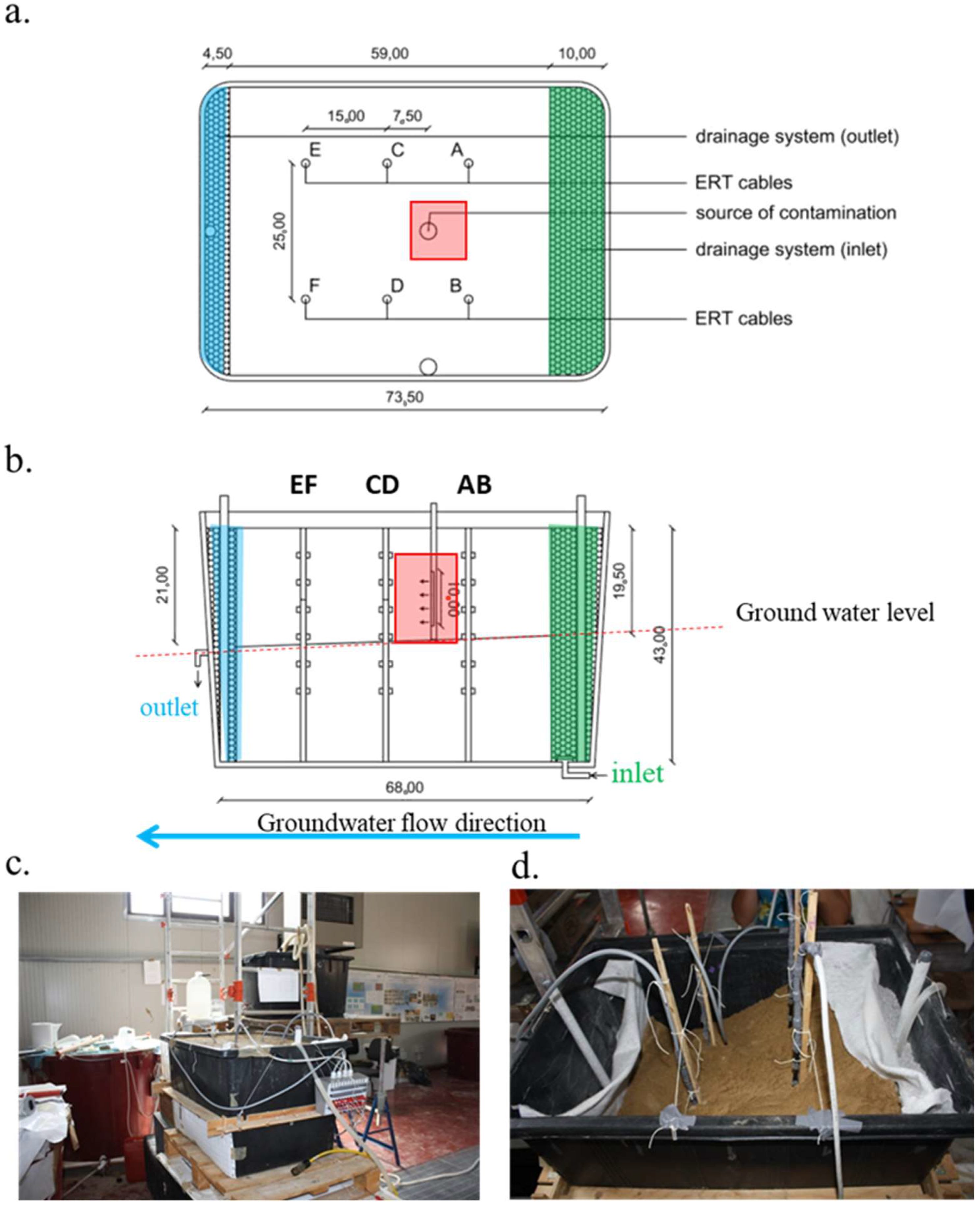
2.2. The Contaminated Analog Aquifer Simulated in Laboratory

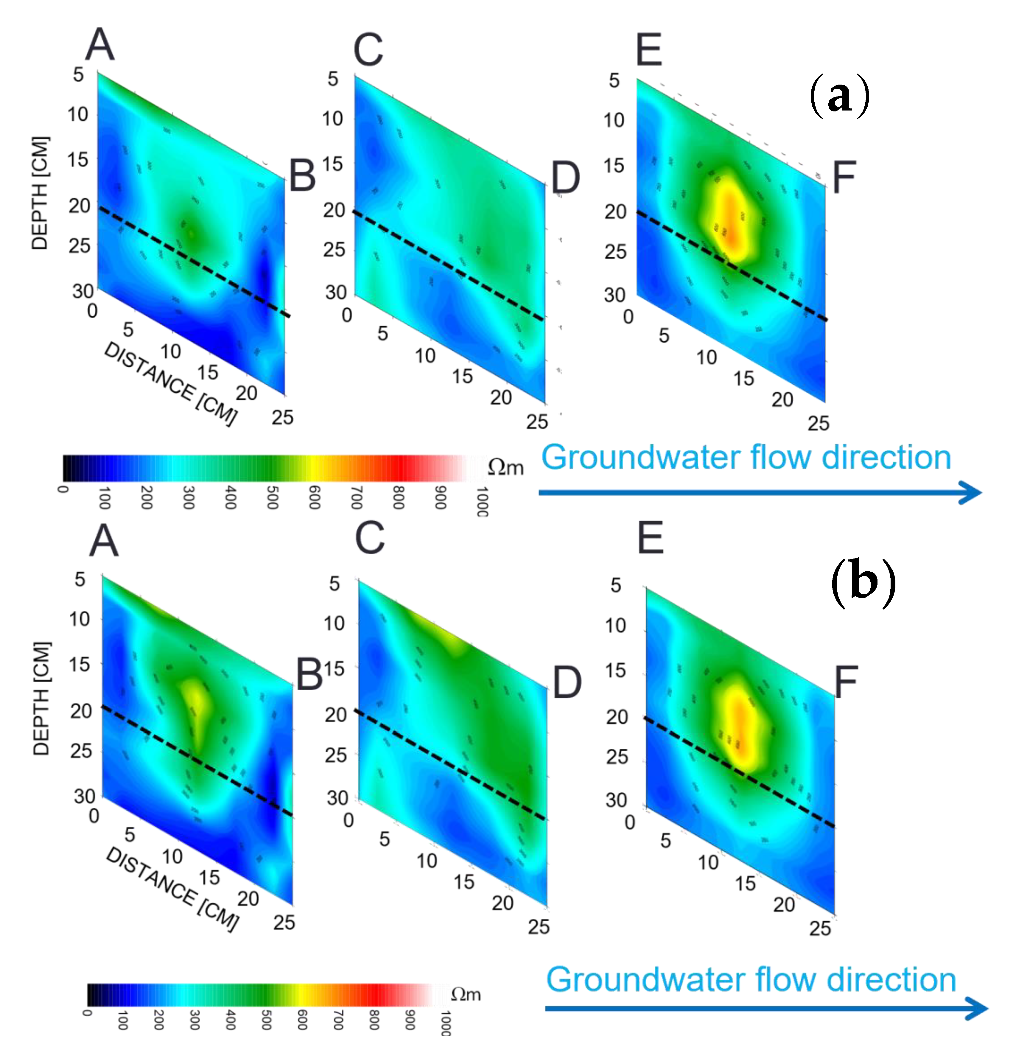
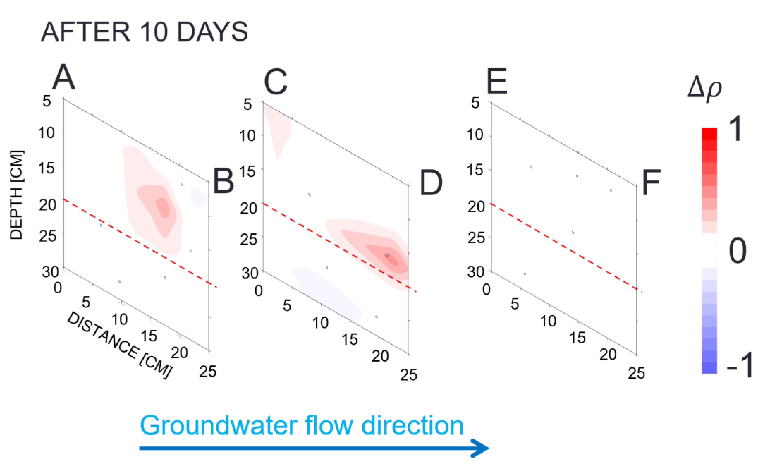
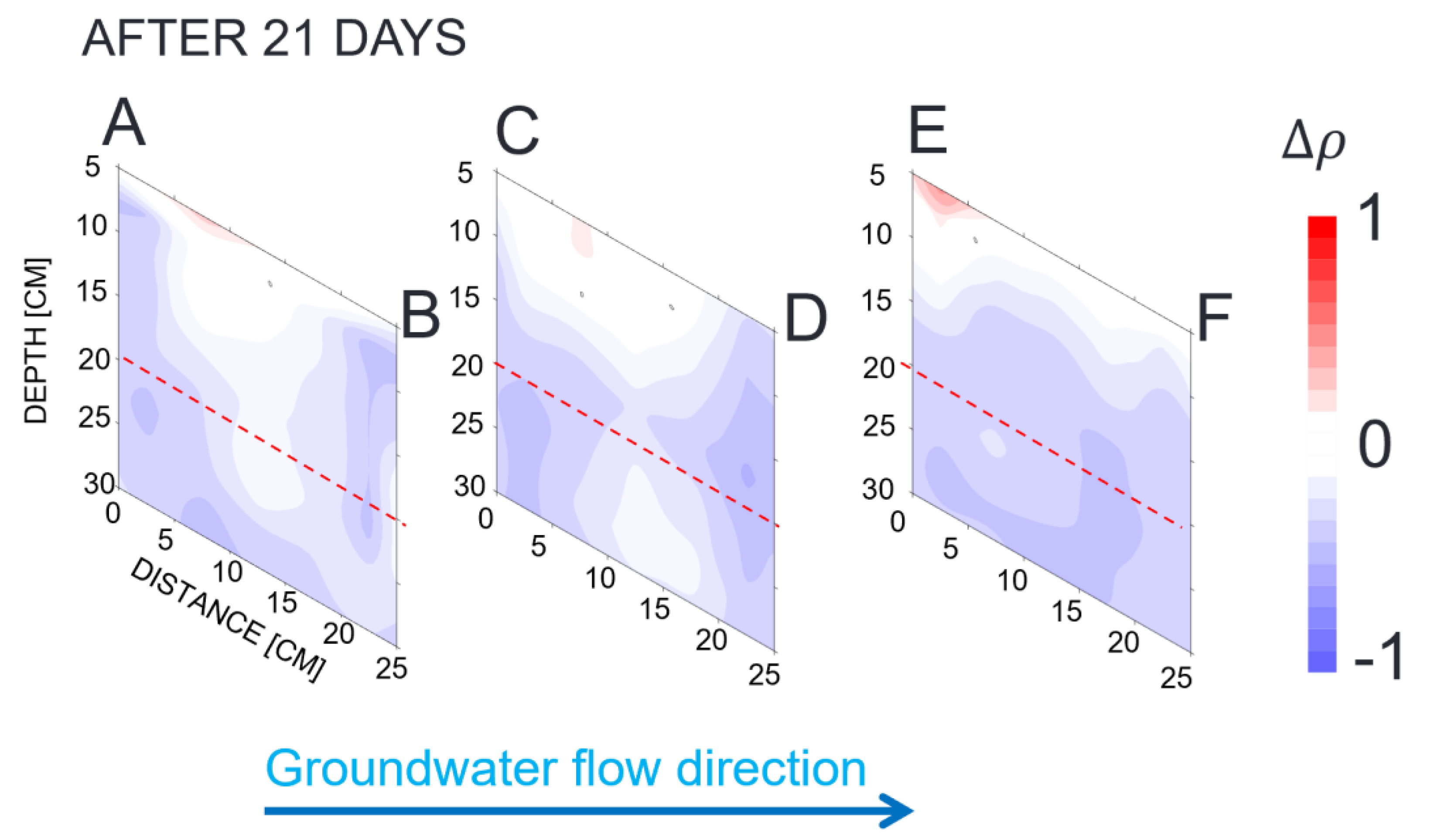
CHERTs were applied to monitor LNAPL in a controlled experiment at the CNR Hydrogeosite Laboratory (Marsico Nuovo, Italy). In detail, contaminant migration and natural attenuation phenomena were monitored in a small-scale aquifer, constituted by both unsaturated and saturated zones. A PVC box (53 cm high × 73.5 cm long × 43 cm deep) filled with fine-grained sand was equipped for the experiment (Figure 1). Silica and homogeneous sand were used to fill the box characterized by the properties described in

Table 1. Chemical analysis, particle size analysis, hydrogeological properties.

Chemical Analysis Results
	SiO2	TiO2	Al2O3	MnO	Fe2O3	MgO	CaO	Na2O	K2O	CO2
%	81.17	0.06	4.75	0.05	0.56	0.13	6.67	0.83	1.15	4.02
Particle Size Analysis
d (mm)	0–0.074	0.75–0.104		0.105–0.149	0.150–0.420		0.421–0.840	0.841–2.000		>2.001
%	0.8	0.03		0.20	14.27		70.67	10.6		3.43
Hydrogeological Properties
dm (mm)				Kmax (m/s)				ρ (%)
0.09				5 × 10−3				35

.

The used sand is a homogeneous quartz-rich sand (95% SiO₂), with a high percentage (86.4 %) of grains between 0.063 mm and 0.125 mm and a medium-high permeability in the order of 10⁻⁵ m/s [52]. A drainage system that allows a water flow composed of two gravel drains located on the opposite sides of the box allows the water flow. Two piezometers have been placed in the drains to monitor water levels over time. The first one is located near the upstream water reserve, while the second one is on the opposite side, where the outlet water flow occurs. The piezometric level was 19.5 cm in the first piezometer and 21 cm in the second one from the surface. Water flow was simulated by injecting tap water (electrical conductivity equal to $0.3\mathrm{mS}/\mathrm{cm})$ through a pump at the bottom right of the tank and draining it off by a hole located on the left side of the box, 26 cm above the box bottom. Figure 1b shows the inlet and outlet points of the tap water. The inlet water level was controlled by an automatic hydraulic system that maintained constant the piezometric gradient (max 1.5 cm) inside the sandbox during the experiment. The flow water rate was 1.8 L per hour. The sandbox was equipped with 6 electrical cables made of 36 stainless steel electrodes spaced 5 cm from each other to allow electrical monitoring of the pollution phenomenon, as shown in Figure 1. The electrodes were arranged in 6 holes drilled into the sand and placed 15 cm apart in the x-direction and 25 cm in the y-direction (Figure 1a), and 5 cm from the bottom (Figure 1b). The steel electrodes were connected to a 96-channel georesistivimeter (Syscal Pro, Iris Instrument Company) through two multichannel cables to perform CHERTs in a time-lapse configuration. The LNAPL spill was simulated using a plastic pipe placed between AB and CD boreholes (as highlighted with a red rectangle in Figure 1b). The plastic pipe was slotted for ten centimeters with lower grooves turned towards CD boreholes direction, so the pollutant was driven by water to the outlet. One liter of common diesel with a density of about 0.83 g/cm³ was used. The contaminant was injected for six hours, and it was monitored for almost a year by continuous resistivity measurements. To better understand physical parameter changes occurring in the sandy body after contamination and to monitor the multiphase fluid migration over time, geophysical measurements were conducted for subsequent steps and different scenarios of water saturation and contamination. At the first stage of the experiment, CHERTs were performed in saturated and uncontaminated conditions to obtain the resistivity distribution before the polluted step as reference resistivity distribution. Then, CHERTs were performed in saturated and unsaturated zones after spillage oil, with the water table located at a fixed depth (19.5 and 21 cm measured from the surface, respectively, in piezometer upstream and downstream). CHERTs were acquired in time-lapse with a cross-borehole azimuthal dipole–dipole array using the “skip one” array with a current and potential dipole separation varying between 0.05 m and 0.15 m. Each acquisition goes on approximately for 13 min, and 252 measurements of apparent resistivity were recorded. The electrical measurements were carried out between boreholes A and B, C and D, and E and F spaced 25 cm from each other. During the experiment, conductivity and temperature measurements of the inlet and output water with the Multi 340i WHW handheld meter probe were carried out to avoid the geophysical results being influenced by variations in the external conditions; moreover, no significant variations were recorded.

3. Results

The electrical behavior of the aquifer immediately before and after the contamination is imaged in Figure 2. The measured apparent resistivity values were inverted using the R2 code [51] using a 2D quadrilateral finite mesh for accounting for current flow towards confined boundaries. For each acquisition, we have performed a data inversion, including a Gaussian error model estimated according to Equation (2). It is worth noting that in uncontaminated conditions (Figure 2a), two different resistivity zones can be distinguished, corresponding to the vadose zone (relative resistive) and water-saturated zone (relative conductive), respectively. Resistivity values range between 150 and 500 Ω*m. The red dashed line indicates the measured groundwater level in the three different sections corresponding to the three areas monitored with CHERTs. As soon as the contamination occurs, a moderate increase in resistivity values is noted only in the section included between boreholes A and B, while the other sections are not affected by strong variations of the electrical behavior (see Figure 2b). The results describe the situation after only 12 h from the leakage, and the absence of the variations, at this stage could be associated with the extremely low mobility of the contaminant. It is also interesting to note the presence of resistive nuclei close to the middle of the sections included between the boreholes A–B and E–F that could suffer some edge effects since they are near to the drainage zone (where gravel material was located to permit the water flow in the aquifer). This effect can be observed in all the tomographies acquired during the experiment.

After these first acquisitions, we have acquired continuous geoelectrical measurements to monitor the contamination phenomena by the CHERTs approach. In order to overcome the problem of side effects and enhance only the electrical resistivity variations related to the studied phenomenon, all the acquired data were plotted in maps of resistivity ratio between uncontaminated and contaminated conditions to determine the relative magnitude of electrical resistivity change, according to the following relationship:

$$\mathsf{\Delta }\mathsf{\rho }=\frac{{\mathsf{\rho }}_{\mathrm{t}}}{{\mathsf{\rho }}_{\mathrm{unc}}}-1$$

(3)

where ${\mathsf{\rho }}_{\mathrm{t}}$ is the inverted resistivity value at t time relative to baseline values and ${\mathsf{\rho }}_{\mathrm{unc}}$ is the inverted resistivity value in the uncontaminated step. Positive values of Δρ mean resistivity increase, while negative values indicate a decrease in electrical resistivity. The resistivity ratio maps allow us to emphasize variations of resistivity values not easily detectable using single resistivity tomography.

The geophysical measurements were carried out for 320 days, and this long experiment allowed us to identify variation patterns of the geoelectrical values with respect to the uncontaminated condition. Therefore, this long monitoring experiment was divided into three main principal phases. In the first phase (phase I), a moderated bulk resistivity increase was observed in the early period after the LNAPL contamination (Figure 3). As expected, some large nuclei are detected in the unsaturated zone where the diesel fuel contamination was spilled. In the beginning, the contaminant still has the free and residual phase, and it floats on the water table. Such behavior is well detected in the electrical resistivity ratio distribution between the boreholes AB and CD, where the values increased. No resistive nuclei are observed between E and F boreholes because the involved area is still uncontaminated.

After this initial bulk resistivity increase lasted 21 days, a variation of the electrical behavior. The new phase (phase II) was characterized by a strong decrease in resistivity values along all the considered sections (Figure 4). A strong variation characterizes the soil, both in the saturated zone and partially in the unsaturated zone. This behavior suggests that a new phenomenon happens in the sandbox, characterized by an abrupt increase in bulk conductivity.

Figure 5 shows a new phase (phase III) that appears after 37 days from the contamination; at this stage, a strong increase in the resistivity values was identified between the boreholes AB. On the contrary, regarding the electrical resistivity sections between CD and EF boreholes, the electrical variations affect the vadose zone. Phase III lasted until the 167th day after the beginning of the experiment. However, the increase in the electrical resistivity values characterizing this phase was inconstant. Up to the 80th day, the increase in the electrical resistivity ratio was well observed. The following period was characterized by decreases and increases in the electrical resistivity distribution; nevertheless, the entire period showed an increase in the resistivity values if compared with the ones recorded in phase II.

After 182 days, a new phase (phase IV), characterized by a constant increase in the conductive behavior of the sandbox, was observed. The decrease in the electrical resistivity ratio affected all the investigated volumes; however, in the unsaturated zone, it was possible to notice a greater variation of the conductive values. This phase was characterized by an increase in conductive values until the end of the experiment (Figure 6), according to the results shown by other authors [6,28,29,30,31,32], that hypothesized that microbial activity might also be the cause of this behavior. After a so-called “period of stress” [53], where microorganisms adapt to the pollutant, hydrocarbons can be deteriorated chemically and be used as a source of carbon and energy [54].

In order to monitor the electrical resistivity behavior, we defined the variation of the electrical resistivity ratio with time. As demonstrated by the results obtained, the effects due of the contaminant that occurs in the sandbox are well observed. For this reason, to simplify the observed phases during the very long monitoring observation, a distribution of the electrical resistivity ratio was defined (Figure 7). The graph was delineated, taking into account the average of the electrical resistivity ratio value calculated for each CHERT section (borehole AB, CB, and EF) obtained each day from the beginning to the end of the experiment. This new value, defined as Mean Resistivity Ratio (MRR), was calculated for all the acquired maps neglecting the values recorded immediately close to the boreholes. This selection was defined to reduce the artifact effects. The variation of MRR clearly identifies the four different phases previously described. We tried to also define two different graphs of the electrical resistivity values recorded in unsaturated and saturated zones, but the observed trends are like the ones shown in Figure 7. Some fluctuations are recorded in each phase, in particular for concerns the phase III, characterized by stronger variations of the values of electrical resistivity.

4. Discussion

The present study confirms the strong link between the characteristic phenomena of hydrocarbon contamination and the geoelectrical signature. Moreover, the CHERT method improves the non-invasive characterization of LNAPL contamination of the media in terms of resolution in depth and quality of the signal. The contamination phenomena hardly influence the physical properties of the simulated aquifer, and in the present case, the capacity of CHERTs to monitor variations induced by diesel spillage in the vadose zone was unequivocally demonstrated. However, the results obtained show high heterogeneity in the electrical behavior due to the used contaminant and its interaction with the aquifer. The complexity shown by the measurements is obviously related to the great variety of degradation processes, including evaporation, dissolution, dispersion, emulsification, adsorption on suspended material, and microbial activity [55] that simultaneously alter the nature of the soil and contaminant. As known, petroleum hydrocarbons provide a distinctive geoelectrical signature that can be well investigated using geophysical techniques. Sorption reactions, in which contamination adheres to the mineral surface [17] or interacts with the mineral surface [56], could partly justify a geo-electrical response, although the electrical behavior is much more complex. Several field tests showed that the smear zone and the capillary fringe, which are the zones most affected by the free-phase hydrocarbon degradation, show higher bulk electrical conductivities, probably due to the products of degradation that may cause an increase in fluid mineralization via the increase in the amount of total dissolved solids, and decreased resistivity [57]. Although we were not able to investigate microbial activity due to their invasive approaches, the similarity of our laboratory results and observations from other studies suggest that changes in geophysical properties of sediment contaminated by hydrocarbons could be referred to as biogeochemical processes associated with microbial growth and activity [30,57,58]. It is worth noting that the physical variations recorded are distributed in the sandbox and are not present as local variations. For this reason, in our opinion, it is more appropriate to discuss a bulk electrical variation identifying four different main phases characterized in turn by a more electrically conductive behavior of the aquifer. The graph of Figure 7, indeed, shows a continuous alternation between relative electrically conductive and resistive distribution that could be associated with different biodegradation processes of the contaminant. The type of contaminant is important in altering the geophysical properties of contaminated sediments, and therefore, phase I is evidently characterized by an increase in the electrical resistivity associated with the poor conductor of the gasoline electricity [57]. This phase continued for 18 days. Even if the contaminated experiment was deficient in sample analysis, each observed phase was clearly detected. Taking into account previous scientific papers, it was possible to identify the gateway of the observed geophysical response. As noted by Serrano et al. [59] in a controlled test, a dramatic decrease in pollutant concentrations occurred in the soil only 18 days after the spill. The reason for this phenomenon has been attributed to the responsibility of evaporation. Due to the evaporation, the contaminant, once volatilized, produces a higher value of electrical conductivity, as observed in our experiment. This phenomenon is also allowed by the fact that the test site is not sealed, and the evaporation of LNAPL is allowed. However, these conditions do not last long. Indeed, phase II lasted from the eighteenth to the thirty-third day, namely just for 14 days. After 40th days from the beginning of the contamination, the electrical resistivity ratio increases, returning to post-contamination values for all the investigated sections. These results highlight that the continuous removal of contaminant mass causes a decrease in bulk conductivity to lower values close to after spill conditions (phase III). Electrical resistivity changes may correspond to variations in data noise level leading to possible numerical artifacts. To overcome this problem, we calculated for each tomography the error model to use for the data inversion according to Equation (2). The end of phase III coincides with an increase in resistive values due to the conclusion of the evaporation process and contaminant displacement into the sand due to groundwater flow. In this phase, some fluctuations are remarkable for the resistivity values. This is due most likely that with time some parts of the LNAPL that coats the sand grain come loose and contributes to creating some local resistive nuclei in the investigated sections. Phase IV of the experiment is characterized by a new electrical bulk conductivity increase, likely due to microbial activities. The most noticeable information is constituted by the increase in the electrical conductibility, probably linked to the variety of degradation processes for the hydrocarbon [55]. The higher bulk conductivity observed at the contaminated locations could result from an increase in the fluid conductivity resulting from enhanced mineral weathering due to metabolic byproducts of microbial degradation. We could infer from these observations that microbial processes may play a significant role in altering the geophysical properties of contaminated sediments. Hence, the influence of biological activity on in situ physical properties can no longer be ignored in the geophysical investigations of contaminated sites [32]. Therefore, the geoelectrical method is a good candidate to evaluate the potential of monitoring the natural attenuation (MNA), which is considered a new cost-effective remediation approach for groundwater at a long-term petroleum hydrocarbon-contaminated site [4]. Finally, the proposed experiment is a starting point approach with the simple contaminant and homogeneous subsoil. Therefore, the next step will consist of petroleum hydrocarbons (PHC), polycyclic aromatic hydrocarbons (PAH), and VOC (Volatile Organic Compound) leakage test in order to collect several referenced data, set useful for field acquisitions and will be focused on the study of the correlation occurring between the concentration of contaminants and detectable magnitude of geoelectrical signal variations.

5. Conclusions

The laboratory test was performed to investigate a simulated contamination leakage in a sandbox by a geoelectrical approach. The geophysical method was able to monitor the saturated and unsaturated subsoil, and a high resolution of the geophysical information was defined with the use of the CHERT approach. Experimental results indicated that subsoil which has been contaminated with hydrocarbon for a long period exhibits a variation of the electrical behavior. Therefore, it was possible to observe that the contamination geophysical response is time-dependent. This suggests that the geophysical approach could be useful for monitoring the effects of induced biodegradation through the repetition of the surveys at different times. From our point of view, this possibility is fundamental for effectively understanding the complex phenomena related to hydrocarbon contamination.

Therefore, the use of geoelectrical techniques at hydrocarbon contaminated sites will become increasingly important not only in the characterization of the subsurface geology and contaminant distribution but also in understanding the impacts of attenuation processes on the subsoil electrical properties. Finally, understanding the relationship between the geoelectrical properties of hydrocarbon-impacted sediments and ongoing physical and biogeochemical processes is a key to the successful application of geoelectrical methods as proxies of these processes. Furthermore, the results of this study suggest that a multidisciplinary approach is fundamental to investigating the physical variations occurring in LNAPL–contaminated sites, and the integration of geophysical measurements with geochemical and biological direct analysis is essentially required.

References

1. Delgado-Rodríguez, O.; Flores-Hernández, D.; Amezcua-Allieri, M.A.; Rosas-Molina, A.; Marín-Córdova, S.; Shevnin, V. Joint interpretation of geoelectrical and volatile organic compounds data: A case study in a hydrocarbons contaminated urban site. Geofís. Int. 2014, 53, 183–198. [Google Scholar] [CrossRef]
2. Rosales, R.M.; Martínez-Pagan, P.; Faz, A.; Moreno-Cornejo, J. Environmental Monitoring Using Electrical Resistivity Tomography (ERT) in the Subsoil of Three Former Petrol Stations in SE of Spain. Water Air Soil Pollut. 2012, 223, 3757–3773. [Google Scholar] [CrossRef]
3. Ciampi, P.; Esposito, C.; Cassiani, G.; Deidda, G.P.; Flores-Orozco, A.; Rizzetto, P.; Chiappa, A.; Bernabei, M.; Gardon, A.; Papini, M.P. Contamination presence and dynamics at a polluted site: Spatial analysis of integrated data and joint conceptual modeling approach. J. Contam. Hydrol. 2022, 248, 104026. [Google Scholar] [CrossRef] [PubMed]
4. Naidu, R.; Nandy, S.; Megharaj, M.; Kumar, R.P.; Chadalavada, S.; Chen, Z.; Bowman, M. Monitored natural attenuation of a long-term petroleum hydrocarbon contaminated sites: A case study. Biodegradation 2012, 23, 881–895. [Google Scholar] [CrossRef]
5. Zanini, A.; Ghirardi, M.; Emiliani, R. A Multidisciplinary Approach to Evaluate the Effectiveness of Natural Attenuation at a Contaminated Site. Hydrology 2021, 8, 101. [Google Scholar] [CrossRef]
6. Sauck, W.A.; Atekwana, E.A.; Nash, M.S. High conductivities associated with an LNAPL plume imaged by integrated geophysical techniques. J. Environ. Eng. Geophys. 1998, 2, 203–212. [Google Scholar]
7. Redman, J.D.; DeRyck, S.M. Monitoring nonaqueous phase liquids in the subsurface with multilevel time domain reflectometry probes. In Proceedings of the Symposium and Workshop on Time Domain Reflectometry in Environmental, Infrastructure and Mining Applications, Evanston, IL, USA, 7–9 September 1994; United States Bureau of Mines: Minneapolis, MN, USA, 1994. [Google Scholar]
8. Balwant, P.L.; Pujari, P.; Dhyani, S.; Bramhanwade, K.; Veligeti, J. Geophysical Methods for Assessing Microbial Processes in Soil: A Critical Review. Indian J. Pure Appl. Phys. 2022, 60, 707–715. [Google Scholar]
9. Daniels, J.J.; Roberts, R.; Vendl, M. Site studies of ground penetrating radar for monitoring petroleum product contaminants. In Proceedings of the 5th EEGS Symposium on the Application of Geophysics to Engineering and Environmental Problems, Oak Brook, IL, USA, 26–29 April 1992; Volume 2, pp. 597–609. [Google Scholar]
10. Campbell, D.L.; Lucius, J.E.; Ellefsen, K.J.; Deszcz-Pan, M. Monitoring of a controlled LNAPL spill using ground-penetrating radar. In 9th EEGS Symposium on the Application of Geophysics to Engineering and Environmental Problems; Bell, R.S., Cramer, M.H., Eds.; European Association of Geoscientists & Engineers: Keystone, CO, USA, 1996; pp. 511–517. [Google Scholar]
11. Giampaolo, V.; Rizzo, E.; Titov, K.; Konosavsky, P.; Laletina, D.; Maineult, A.; Lapenna, V. Self-potential monitoring of a crude oil-contaminated site (Trecate, Italy). Environ. Sci. Pollut. Res. 2014, 21, 8932–8947. [Google Scholar] [CrossRef]
12. Ntarlagiannis, D.; Yee, N.; Slater, L. On the low-frequency electrical polarization of bacterial cells in sands. Geophys. Res. Lett. 2005, 32, L24402. [Google Scholar] [CrossRef]
13. Ntarlagiannis, D.; Williams, K.H.; Slater, L.; Hubbard, S. Low-frequency electrical response to microbial induced sulfide precipitation. J. Geophys. Res. 2005, 110, G02009. [Google Scholar] [CrossRef]
14. Davis, C.A.; Atekwana, E.; Atekwana, E.; Slater, L.D.; Rossbach, S.; Mormile, M.R. Microbial growth and biofilm formation in geologic media is detected with complex conductivity measurements. Geophys. Res. Lett. 2006, 33, L18403. [Google Scholar] [CrossRef]
15. Guéguen, Y.; Palciauskas, V. Introduction to the Physics of Rocks; Princeton University Press: Princeton, NJ, USA, 1994. [Google Scholar]
16. Schön, J.H. Physical Properties of Rocks: Fundamentals and Principles of Petrophysics. In Handbook of Geophysical Exploration: Seismic Exploration; Elsevier: Oxford, UK, 2004; Volume 18. [Google Scholar]
17. Lesmes, D.P.; Friedman, S. Relationships between the electrical and hydrogeological properties of rocks and soils. In Hydrogeophysics; Rubin, Y., Hubbard, S., Eds.; Springer: Dordrecht, The Netherlands, 2005. [Google Scholar]
18. Chambers, J.E.; Wilkinson, P.B.; Wealthall, G.P.; Loke, M.H.; Dearden, R.; Wilson, R.; Allen, D.; Ogilvy, R.D. Hydrogeophysical imaging of deposit heterogeneity and groundwater chemistry changes during DNAPL source zone bioremediation. J. Contam. Hydrol. 2010, 118, 43–61. [Google Scholar] [CrossRef] [PubMed] [Green Version]
19. Mazàc, O.; Kelly, W.E.; Landa, I. A hydrogeophysical model for relations between electrical and hydraulic properties of aquifers. J. Hydrol. 1985, 79, 1–19. [Google Scholar] [CrossRef]
20. Lien, B.K.; Enfield, C.G. Delineation of subsurface hydrocarbon contaminated distribution using a direct push resistivity method. J. Environ. Eng. Geophys. 1998, 2–3, 173–179. [Google Scholar]
21. Benson, A.K.; Payne, K.L.; Stubben, M.A. Mapping groundwater contamination using dc resistivity and, VLF geophysical methods—A case study. Geophysics 1997, 62, 80–86. [Google Scholar] [CrossRef]
22. Olhoeft, G.R. Direct detection of hydrocarbon and organic chemicals with ground penetrating radar and complex resistivity. In Proceedings of the NWWA/API Conference Petroleum Hydrocarbons and Organic Chemicals in Ground Water-Prevention, Detection and Restoration, Dublin, OH, USA, 12–14 November 1986; pp. 284–305. [Google Scholar]
23. King TV, V.; Olhoeft, G.R. Mapping organic contamination by detection of clay-organic processes. In Proceedings of the AGWSE/NWWA/API, Conference on Petroleum Hydrocarbons and Organic Chemicals in Ground Water-Prevention, Detection and Restoration, Houston, TX, USA, 15–17 November 1989; pp. 627–640. [Google Scholar]
24. DeRyck, S.M.; Redman, J.D.; Annan, A.P. Geophysical monitoring of controlled kerosene spill. In Proceedings of the Symposium on the Application of Geophysics to Engineering and Environmental Problems (SAGEEP), San Diego, CA, USA, 18–22 April 1993; pp. 5–19. [Google Scholar]
25. Redman, J.D.; DeRyck, S.M.; Annan, A.P. Detection of LNAPL pools with GPR, Theoretical modeling and surveys of a controlled spill. In Proceedings of the Fifth International Conference on Ground penetrating Radar (GPR’94), Kitchener, ON, Canada, 12–16 June 1994; pp. 1283–1294. [Google Scholar]
26. Endres, A.L.; Redman, J.D. Modelling the electrical properties of porous rocks and soils containing immiscible contaminants. J. Environ. Eng. Geophys. 1996, 105–112. [Google Scholar] [CrossRef]
27. Che-Alota, V.; Atekwana, E.A.; Sauck, W.A.; Werkema, D.D. Temporal Geophysical Signatures from Contaminant-Mass Remediation. Geophysics 2009, 4, B113–B123. [Google Scholar] [CrossRef]
28. Werkema, D.D.; Atekwana, E.A.; Anthony, L.E.; Sauck, W.A.; Cassidy, D.P. Investigating the geoelectrical response of hydrocarbon contamination undergoing biodegradation. Geophys. Res. Lett. 2003, 30, 49-1–49-4. [Google Scholar] [CrossRef]
29. Atekwana, E.A.; Atekwana, E.A.; Legall, F.D.; Krishnamurthy, R.V. Field evidence for geophysical detection of subsurface zones of enhanced microbial activity. Geophys. Res. Lett. 2004, 31, L23603. [Google Scholar] [CrossRef]
30. Atekwana, E.A.; Atekwana, E.A.; Rowe, R.S.; Werkema, D.D.; Legall, F.D. Total dissolved solids in groundwater and its relationship to bulk electrical conductivity of soils contaminated with hydrocarbon. J. Appl. Geophys. 2004, 56, 281–294. [Google Scholar] [CrossRef]
31. Atekwana, E.A.; Atekwana, E.A.; Werkema, D.D.; Allen, J.P.; Smart, L.A.; Duris, J.W.; Cassidy, D.; PSauck, W.A.; Rossbach, S. Evidence for microbial enhanced electrical conductivity in hydrocarbon-contaminated sediments. Geophys. Res. Lett. 2004, 31, L23501. [Google Scholar] [CrossRef]
32. Atekwana, E.A.; Atekwana, E.A.; Legall, F.D.; Krishnamurthy, R.V. Biodegradation and mineral weathering controls on bulk electrical conductivity in a shallow hydrocarbon contaminated aquifer. J. Contam. Hydrol. 2005, 80, 149–167. [Google Scholar] [CrossRef] [PubMed]
33. Cassiani, G.; Binley, A.; Kemna, A.; Wehrer, M.; Orozco, A.F.; Deiana, R.; Boaga, J.; Rossi, M.; Dietrich, P.; Werban, U.; et al. Noninvasive characterization of the Trecate (Italy) crude-oil contaminated site: Links between contamination and geophysical signals. Environ. Sci. Pollut. Res. 2014, 21, 8914–8931. [Google Scholar] [CrossRef] [PubMed]
34. Vergnano, A.; Raffa, C.M.; Godio, A.; Chiampo, F. Electromagnetic Properties Monitoring to Detect Different Biodegradation Kinetics in Hydrocarbon-Contaminated Soil. Soil Syst. 2022, 6, 48. [Google Scholar] [CrossRef]
35. Revil, A.; Atekwana, E.; Zhang, C.; Jardani, A.; Smith, S. A new model for the spectral induced polarization signature of bacterial growth in porous media. Water Resour. Res. 2012, 48. [Google Scholar] [CrossRef]
36. Power, C.; Gerhard, J.I.; Tsourlos, P.; Soupios, P.; Simyrdanis, K.; Karaoulis, M. Improved time-lapse electrical resistivity tomography monitoring of dense non-aqueous phase liquids with surface-to-horizontal borehole arrays. J. Appl. Geophys. 2015, 112, 1–13. [Google Scholar] [CrossRef]
37. Masy, T.; Caterina, D.; Tromme, O.; Lavigne, B.; Thonart, P.; Hiligsmann, S.; Nguyen, F. Electrical resistivity tomography to monitor enhanced biodegradation of hydrocarbons with Rhodococcus erythropolis T902.1 at a pilot scale. J. Contam. Hydrol. 2016, 184, 1–13. [Google Scholar] [CrossRef]
38. Nazifi, H.M.; Gülen, L.; Gürbüz, E.; Pekşen, E. Time-lapse electrical resistivity tomography (ERT) monitoring of used engine oil contamination in laboratory setting. J. Appl. Geophys. 2022, 197, 104531. [Google Scholar] [CrossRef]
39. De Groot-Hedlin, C.D.; Constable, S.C. Occam’s inversion to generate smooth, two-dimensional models from magnetotelluric data. Geophysics 1990, 55, 1613–1624. [Google Scholar] [CrossRef]
40. Daily, W.D.; Ramirez, A.L.; LaBrecque, D.J.; Nitao, J. Electrical resistivity tomography of vadose water movement. Water Resour. Res. 1992, 28, 1429–1442. [Google Scholar] [CrossRef]
41. Binley, A.; Cassiani, G.; Middleton, R.; Winship, P. Vadose zone model parameterisation using cross-borehole radar and resistivity imaging. J. Hydrol. 2002, 267, 147–159. [Google Scholar] [CrossRef]
42. Giampaolo, V.; Rizzo, E.; Straface, S.; Votta, M. Hydrogeophysics techniques for the characterization of a heterogeneous aquifer. Boll. Geofis. Teor. Appl. 2011, 52, 595–606. [Google Scholar]
43. Rizzo, E.; Giampaolo, V.; Capozzoli, L.; De Martino, G.; Romano, G.; Santilano, A.; Manzella, A. 3D deep geoelectrical exploration in the Larderello geothermal sites (Italy). Phys. Earth Planet. Inter. 2022, 329–330, 106906. [Google Scholar] [CrossRef]
44. Wilkinson, P.B.; Chambers, J.E.; Meldrum, P.I.; Ogilvy, R.D.; Caunt, S. Optimization of array configurations and panel combinations for the detection and imaging of abandoned mineshafts using 3D cross-hole electrical resistivity tomography. J. Environ. Eng. Geophys. 2006, 11, 213–221. [Google Scholar] [CrossRef] [Green Version]
45. Kemna, A.; Vanderborght, J.; Kulessa, B.; Vereecken, H. Imaging and characterisation of subsurface solute transport using electrical resistivity tomography (ERT) and equivalent transport models. J. Hydrol. 2002, 267, 125–146. [Google Scholar] [CrossRef]
46. Kremera, T.; Vieira, C.; Maineult, A. ERT monitoring of gas injection into water saturated sands: Modelling and inversion of cross-hole laboratory data. J. Appl. Geophys. 2018, 158, 11–28. [Google Scholar] [CrossRef]
47. Wilkinson, P.B.; Chambers, J.E.; Lelliott, M.; Wealthall, P.; Ogilvy, R.D. Extreme sensitivity of cross-hole electrical resistivity tomography measurements to geometric errors. Geophys. J. Int. 2008, 173, 49–62. [Google Scholar] [CrossRef]
48. Chambers, J.E.; Gunn, D.A.; Wilkinson, P.B.; Ogilvy, R.D.; Ghataora, G.S.; Burrow, M.P.N.; Smith, R.T. Non-invasive Time-lapse Imaging of Moisture Content Changes in Earth Embankments Using Electrical Resistivity Tomography (ERT). In Advances in Transportation Geotechnics; CRC Press-Taylor & Francis Group: Boca Raton, FL, USA, 2008; pp. 475–480. [Google Scholar]
49. Slater, L.; Binley, A.; Daily, W.D.; Johnson, R. Cross-hole electrical imaging of a controlled saline tracer injection. J. Appl. Geophys. 2000, 44, 85–102. [Google Scholar] [CrossRef]
50. LaBrecque, D.J.; Milleto, M.; Daily, W.; Ramirez, A.; Owen, E. The effects of noise on Occam’s inversion of resistivity tomography data. Geophysics 1996, 61, 538–548. [Google Scholar] [CrossRef]
51. Binley, A. R2 Version 3.1 Manual. Lancaster. 2016. Available online: http://www.es.lancs.ac.uk/people/amb/Freeware/R2/R2.htm (accessed on 28 April 2022).
52. Straface, S.; Rizzo, E.; Chidichimo, F. Estimation of hydraulic conductivity and water table map in a large-scale laboratory model by means of the self-potential method. J. Geophys. Res. 2010, 115, B06105. [Google Scholar] [CrossRef]
53. Baran, S.; Bielińska, J.E.; Oleszczuk, P. Enzymatic activity in an airfield soil polluted with polycyclic aromatic hydrocarbons. Geoderma 2004, 118, 221–232. [Google Scholar] [CrossRef]
54. Wang, C.H.; Yu, C.Y.; Su, S.W. High resistivities associated with a newly formed LNAPL plume imaged by geoelectric techniques—A case study. J. Chin. Inst. Eng. 2007, 30, 53–56. [Google Scholar]
55. Atekwana, E.A.; Slater, L.D. Biogeophysics: A new frontier in Earth science research. Rev. Geophys. 2009, 47, RG4004. [Google Scholar] [CrossRef]
56. Vaudelet, P.; Revil, A.; Schmutz, M.; Franceschi, M.; Bégassat, P. Induced polarization signature of the presence of copper in saturated sands. Water Resour. Res. 2011, 47, W02526. [Google Scholar] [CrossRef]
57. Gomaa, M.M.; Elnasharty, M.M.M.; Rizzo, E. Electrical properties speculation of contamination by water and gasoline on sand and clay composite. Arab. J. Geosci. 2019, 12, 581. [Google Scholar] [CrossRef]
58. Abdel Aal, G.Z.; Atekwana, E.A.; Slater, L.D.; Atekwana, E.A. Effects of microbial processes on electrolytic and interfacial electrical properties of unconsolidated sediments. Geophys. Res. Lett. 2004, 31, L12505. [Google Scholar] [CrossRef]
59. Serrano, A.; Gallego, M.; Gonzalez, J.L.; Tejada, M. Natural attenuation of diesel aliphatic hydrocarbons in contaminated agricultural soil. Environ. Pollut. 2008, 151, 494–502. [Google Scholar] [CrossRef]
Figure 1. Plan of the test site with indications of the three borehole couples (AB-CD-EF) (a); vertical section of the box with contamination zone highlighting (red rectangle) and identification of the recharge and discharge systems (green and blue rectangle, respectively) (b); photo of laboratory test site (c) and detail of the geoelectrical boreholes used for the experiment (d).
Geosciences 12 00360 g001
Figure 2. Resistivity maps acquired in uncontaminated conditions (a) and after 12 h from the contamination (b). The sections describe the resistivity behavior measured with CHERTs between the three sections enclosed between the three couples of geoelectrical boreholes.
Geosciences 12 00360 g002
Figure 3. CHERTs after 10 days from the contamination event. A moderate increase in resistivity values can be appreciated in the vadose zone above the groundwater table.
Geosciences 12 00360 g003
Figure 4. CHERTs after 21 days from the contamination. It is clear a sharp increase in conductivity values concerning the saturated zone below the groundwater table.
Geosciences 12 00360 g004
Figure 5. CHERTs obtained after 81 days from the contamination. A resistive behavior characterizes more strongly the section near the contamination source, as highlighted by the vertical sections A–B and C–D.
Geosciences 12 00360 g005
Figure 6. CHERTs obtained after 320 days from the contamination. The contamination generates evidence of conductive behavior for all the investigated sections.
Geosciences 12 00360 g006
Figure 7. Temporal distribution of resistivity maps mean value recorded between the built-up boreholes with individuation of the hypothesized phases.
Geosciences 12 00360 g007