
Cosmogenic Exposure Dating (36Cl) of Landforms on Jan Mayen, North Atlantic, and the Effects of Bedrock Formation Age Assumptions on 36Cl Ages

 , , , and
Abstract
:1. Introduction
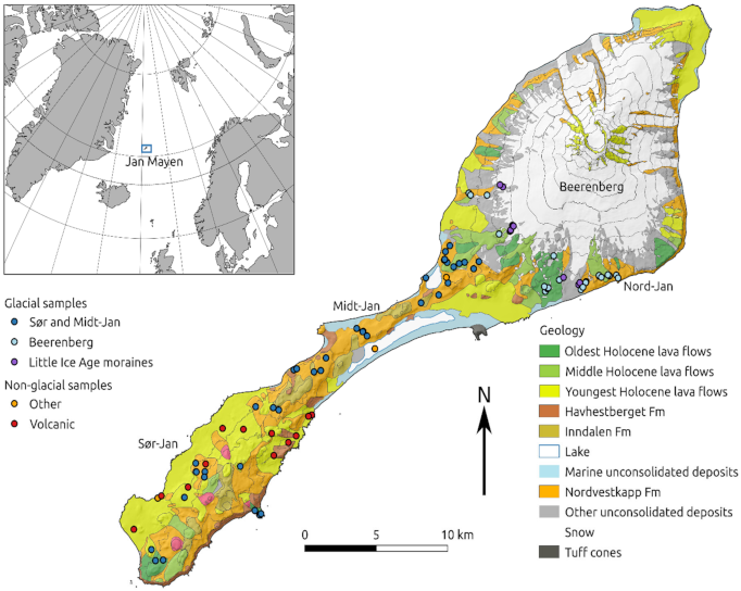
Study Area
2. Materials and Methods
2.1. Sampling Strategy
2.2. Sample Treatment and Measurements
2.3. Calculations
2.4. Radiocarbon Dating
3. Results and Interpretations
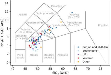
3.1. Geochemistry
3.2. Radiocarbon Date
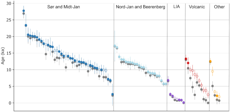
3.3. Cosmogenic Nuclide Surface Exposure Age Dating
4. Discussion
4.1. Evaluation of General Uncertainties
4.2. Influence of Young Bedrock
4.3. Deglaciation Pattern
5. Conclusions
- In this study, we present 89 cosmogenic exposure ages (36Cl) from Jan Mayen, most of them dating either the deglaciation (n = 73) or postglacial volcanic events (n = 11) on the island.
- Based on the range of exposure ages at each location, large-scale deglaciation on Jan Mayen began ~20 ka and continued until 5.7 ka, after which the glaciers appear to have retreated inside the Little Ice Age moraines.
- The exposure ages on Jan Mayen were calculated using an updated version of CRONUScalc to account for the young bedrock formation ages at the site. Although the formation age assumption does not significantly affect most samples (n = 64), a number of exposure ages change substantially (n = 25) depending on the rock formation age assumed for the sample. On Jan Mayen, the most appropriate assumption for rock formation age varied by sample group: for samples dating volcanic activity, formation age should be assumed equal to the exposure age, whereas a rock formation age of 50 ka was used for the remaining samples.
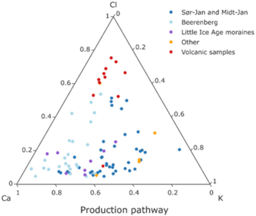
- We recommend not assuming equilibrium conditions when calculating 36Cl ages on rocks that meet the following criteria: (i) known young rock formation ages, and (ii) potentially susceptible composition, specifically high native Cl, or high U and/or Th concentrations that are likely to occur in volcanic rocks. Young exposure age samples will be particularly affected because of the large mismatch between expected equilibrium conditions and measured concentrations.
Supplementary Materials
Author Contributions
Funding
Data Availability Statement
Conflicts of Interest
References
- Lyså, A.; Larsen, E.A.; Anjar, J.; Akçar, N.; Ganerød, M.; Hiksdal, A.; Van Der Lelij, R.; Vockenhuber, C. The last glaciation of the Arctic volcanic island Jan Mayen. Boreas 2021, 50, 6–28. [Google Scholar] [CrossRef]
- Larsen, E.; Lyså, A.; Höskuldsson, Á.; Davidsen, J.G.; Nadeau, M.J.; Power, M.; Tassis, G.; Wastegård, S. A dated volcano-tectonic deformation event in Jan Mayen causing landlocking of Arctic charr. J. Quat. Sci. 2021, 36, 180–190. [Google Scholar] [CrossRef]
- Dallmann, W.K. Bergrunnsgeologi Jan Mayen. In Natur og Kulturmiljøet på Jan Mayen—Med en Vurdering av Verneverdier, Kunnskapsbehov og Forvaltning; Gabrielsen, G.W., Brekke, B., Alsos, I.G., Hansen, J.R., Eds.; Norsk Polarinstitutt Meddelelser: Tromso, Norway, 1997; Volume 144, p. 35. [Google Scholar]
- Gosse, J.C.; Phillips, F.M. Terrestrial in situ cosmogenic nuclides: Theory and application. Quat. Sci. Rev. 2001, 20, 1475–1560. [Google Scholar] [CrossRef]
- Marrero, S.M.; Phillips, F.M.; Borchers, B.; Lifton, N.; Aumer, R.; Balco, G. Cosmogenic nuclide systematics and the CRONUScalc program. Quat. Geochronol. 2016, 31, 160–187. [Google Scholar] [CrossRef] [Green Version]
- Phillips, F.M.; Plummer, M.A. Chloe: A Program for Interpreting in-Situ Cosmogenic Nuclide Data for Surface Exposure Dating and Erosion Studies. Radiocarbon 1996, 38, 98–99. [Google Scholar]
- Schimmelpfennig, I.; Benedetti, L.; Finkel, R.; Pik, R.; Blard, P.-H.; Bourlès, D.; Burnard, P.; Williams, A. Sources of in-situ 36Cl in basaltic rocks. Implications for calibration of production rates. Quat. Geochronol. 2009, 4, 441–461. [Google Scholar] [CrossRef]
- Parmelee, D.E.; Kyle, P.R.; Kurz, M.D.; Marrero, S.M.; Phillips, F.M. A new Holocene eruptive history of Erebus volcano, Antarctica using cosmogenic 3He and 36Cl exposure ages. Quat. Geochronol. 2015, 30, 114–131. [Google Scholar] [CrossRef] [Green Version]
- Marrero, S.; Phillips, F.M.; Caffee, M.W.; Gosse, J.C. CRONUS-Earth cosmogenic 36Cl calibration. Quat. Geochronol. 2016, 31, 199–219. [Google Scholar] [CrossRef] [Green Version]
- Cromwell, G.; Tauxe, L.; Staudigel, H.; Constable, C.G.; Koppers, A.A.P.; Pedersen, R.-B. In search of long-term hemispheric asymmetry in the geomagnetic field: Results from high northern latitudes (Dataset). Geochem. Geophys. Geosyst. 2013, 14, 3234–3249. [Google Scholar] [CrossRef] [Green Version]
- White, C.A. Petrology and Mineral Chemistry of Some Jan Mayen Volcanics. Master’s Thesis, State University of New York at Albany, Albany, NY, USA, 1979. [Google Scholar]
- Anda, E.O.O.; Mangerud, J.A.N. Late Holocene Glacier Variations and Climate at Jan Mayen. Polar Res. 1985, 3, 129–140. [Google Scholar] [CrossRef]
- Larsen, E. (Geological Survey of Norway, Trondheim, Norway). Personal communication, 2021. [Google Scholar]
- Imsland, P. The Volcanic Eruption on Jan Mayen, January 1985: Interaction between a Volcanic Island and a Fracture Zone. J. Volcanol. Geotherm. Res. 1986, 28, 45–53. [Google Scholar] [CrossRef]
- Gjelsvik, T. Volcano on Jan Mayen Alive Again. Nat. Cell Biol. 1970, 228, 352. [Google Scholar] [CrossRef]
- Sylvester, A.G. History and surveillance of volcanic activity on Jan Mayen island. Bull. Volcanol. 1975, 39, 313–335. [Google Scholar] [CrossRef]
- Gjerløw, E. Holocene Volcanic Activity and Hazards of Jan Mayen, North-Atlantic. Ph.D. Thesis, University of Bergen, Bergen, Norway, 2018. [Google Scholar]
- Maaloe, S.; Sorensen, I.; Hertogen, J. The Trachybasaltic Suite of Jan Mayen. J. Pet. 1986, 27, 439–466. [Google Scholar] [CrossRef]
- Elmore, D.; Ma, X.; Miller, T.; Mueller, K.; Perry, M.; Rickey, F.; Sharma, P.; Simms, P.; Lipschütz, M.; Vogt, S. Status and plans for the PRIME Lab AMS facility. Nucl. Instrum. Methods Phys. Res. Sect. B Beam Interact. Mater. Atoms 1997, 123, 69–72. [Google Scholar] [CrossRef]
- Ivy-Ochs, S.; Synal, H.-A.; Roth, C.; Schaller, M. Initial results from isotope dilution for Cl and 36Cl measurements at the PSI/ETH Zurich AMS facility. Nucl. Instrum. Methods Phys. Res. Sect. B Beam Interact. Mater. Atoms 2004, 223–224, 623–627. [Google Scholar] [CrossRef]
- Desilets, D.; Zreda, M.; Almasi, P.F.; Elmore, D. Determination of cosmogenic 36Cl in rocks by isotope dilution: Innovations, validation and error propagation. Chem. Geol. 2006, 233, 185–195. [Google Scholar] [CrossRef]
- Stone, J.; Allan, G.; Fifield, L.; Cresswell, R. Cosmogenic chlorine-36 from calcium spallation. Geochim. Cosmochim. Acta 1996, 60, 679–692. [Google Scholar] [CrossRef]
- Ivy-Ochs, S.; Poschinger, A.; Synal, H.-A.; Maisch, M. Surface exposure dating of the Flims landslide, Graubünden, Switzerland. Geomorphology 2009, 103, 104–112. [Google Scholar] [CrossRef]
- Zreda, M.G.; Phillips, F.M.; Elmore, D.; Kubik, P.W.; Sharma, P.; Dorn, R.I. Cosmogenic chlorine-36 production rates in terrestrial rocks. Earth Planet. Sci. Lett. 1991, 105, 94–109. [Google Scholar] [CrossRef]
- Synal, H.-A.; Bonani, G.; Döbeli, M.; Ender, R.; Gartenmann, P.; Kubik, P.; Schnabel, C.; Suter, M. Status report of the PSI/ETH AMS facility. Nucl. Instrum. Methods Phys. Res. Sect. B Beam Interact. Mater. Atoms 1997, 123, 62–68. [Google Scholar] [CrossRef]
- Christl, M.; Vockenhuber, C.; Kubik, P.; Wacker, L.; Lachner, J.; Alfimov, V.; Synal, H.-A. The ETH Zurich AMS facilities: Performance parameters and reference materials. Nucl. Instrum. Methods Phys. Res. Sect. B Beam Interact. Mater. Atoms 2013, 294, 29–38. [Google Scholar] [CrossRef]
- Vockenhuber, C.; Miltenberger, K.-U.; Synal, H.-A. 36Cl measurements with a gas-filled magnet at 6 MV. Nucl. Instrum. Nucl. Instrum. Methods Phys. Res. Sect. B Beam Interact. Mater. Atoms 2019, 455, 190–194. [Google Scholar] [CrossRef]
- Moore, A.K.; Granger, D.E. Calibration of the production rate of cosmogenic 36Cl from Fe. Quat. Geochronol. 2019, 51, 87–98. [Google Scholar] [CrossRef]
- Stone, J.O.; Fifield, K.; Vasconcelos, P.M. Terrestrial Chlorine-36 Production from Spallation of Iron. In Proceedings of the 10th International Conference on Accelerator Mass Spectrometry, Berkeley, CA, USA, 5–10 September 2005. [Google Scholar]
- Marrero, S.M.; Phillips, F.M.; Caffee, M.; Gosse, J.C. Corrigendum to “Cronus-Earth Cosmogenic 36Cl Calibration” [Quat. Geochronol. 31 (2016) 199–219]. Quat. Geochronol. 2021, 61, 101130. [Google Scholar] [CrossRef]
- Leontaritis, A.D. The Late Quaternary Glacial History of Greece. Ph.D. Thesis, Harokopio University of Athens, Athens, Greece, 2021. [Google Scholar]
- Moore, A. (Purdue University, West Lafayette, IN, USA). Personal communication, 2020. [Google Scholar]
- Lal, D. Cosmic ray labeling of erosion surfaces: In situ nuclide production rates and erosion models. Earth Planet. Sci. Lett. 1991, 104, 424–439. [Google Scholar] [CrossRef]
- Stone, J.O. Air pressure and cosmogenic isotope production. J. Geophys. Res. Space Phys. 2000, 105, 23753–23759. [Google Scholar] [CrossRef]
- Licciardi, J.; Denoncourt, C.; Finkel, R. Cosmogenic 36Cl production rates from Ca spallation in Iceland. Earth Planet. Sci. Lett. 2008, 267, 365–377. [Google Scholar] [CrossRef]
- Reimer, P.J.; Austin, W.E.N.; Bard, E.; Bayliss, A.; Blackwell, P.G.; Ramsey, C.B.; Butzin, M.; Cheng, H.; Edwards, R.L.; Friedrich, M.; et al. The Intcal20 Northern Hemisphere Radiocarbon Age Calibration Curve (0–55 Cal Kbp). Radiocarbon 2020, 62, 725–757. [Google Scholar] [CrossRef]
- Le Maitre, R.; Streckeisen, A.; Zanettin, B.; Le Bas, M.; Bonin, B.; Bateman, P. (Eds.) Igneous Rocks: A Classification and Glossary of Terms: Recommendations of the International Union of Geological Sciences Subcommission on the Systematics of Igneous Rocks, 2nd ed.; Cambridge University Press: Cambridge, UK, 2002. [Google Scholar]
- Phillips, F.M.; Stone, W.D.; Fabryka-Martin, J.T. An improved approach to calculating low-energy cosmic-ray neutron fluxes near the land/atmosphere interface. Chem. Geol. 2001, 175, 689–701. [Google Scholar] [CrossRef]
- Principato, S.M.; Geirsdóttir, Á.; Jóhannsdóttir, G.E.; Andrews, J.T. Late Quaternary Glacial and Deglacial History of Eastern Vestfirdir, Iceland Using Cosmogenic Isotope (36cl) Exposure Ages and Marine Cores. J. Quat. Sci. 2006, 21, 271–285. [Google Scholar] [CrossRef]


| Pathway | Production Rate (at 36Cl g−1 y−1) | % Change From v2.1 |
|---|---|---|
| Ca—Spallation | 51.686 ± 3.3 | −0.0003 |
| K—Spallation | 150.996 ± 10 | 0.66 |
| Pf(0) | 647.705 ± 231 | 0.37 |
| Name | Latitude WGS84 | Longitude WGS84 | Elevation | Equilibrium Assumption * (Equil.) | Formation Age = 564 ka | Formation Age = 250 ka | Formation Age = 50 ka | Formation Age = Exposure Age (Young Rock) | ||||||||||
|---|---|---|---|---|---|---|---|---|---|---|---|---|---|---|---|---|---|---|
| [dd] | [dd] | [m] | Age [ka] | Unc (ext) | Unc (int) | Age [ka] | Unc (ext) | Unc (int) | Age [ka] | Unc (ext) | Unc (int) | Age [ka] | Unc (ext) | Unc (int) | Age [ka] | Unc (ext) | Unc (int) | |
| Glacial samples–Sør Jan and Midt Jan | ||||||||||||||||||
| JM2014-01 | 70.9751 | −8.6210 | 114 | 19.8 | 1.6 | 1.2 | 19.9 | 1.6 | 1.2 | 19.9 | 1.6 | 1.2 | 20.0 | 1.6 | 1.2 | 20.0 | 1.6 | 1.2 |
| JM2014-18 | 71.0144 | −8.4514 | 52 | 7.7 | 1.6 | 0.8 | 8.3 | 1.6 | 0.8 | 8.9 | 1.7 | 0.8 | 9.6 | 1.8 | 0.8 | 9.8 | 1.9 | 0.8 |
| JM2014-19 | 71.0104 | −8.4334 | 119 | 13.4 | 1.1 | 0.9 | 13.4 | 1.1 | 0.9 | 13.4 | 1.1 | 0.9 | 13.5 | 1.1 | 0.9 | 13.5 | 1.1 | 0.9 |
| JM2014-20 | 71.0123 | −8.4226 | 144 | 11.6 | 1.2 | 0.9 | 11.7 | 1.2 | 0.9 | 11.7 | 1.2 | 0.9 | 11.8 | 1.2 | 0.9 | 11.8 | 1.2 | 0.9 |
| JM2014-21 | 71.0129 | −8.4121 | 162 | 19.0 | 2.4 | 2.2 | 19.0 | 2.4 | 2.2 | 19.1 | 2.4 | 2.2 | 19.1 | 2.4 | 2.2 | 19.1 | 2.4 | 2.2 |
| JM2014-22 | 71.0227 | −8.4404 | 55 | 11.2 | 1.2 | 0.8 | 11.5 | 1.3 | 0.8 | 12.0 | 1.3 | 0.9 | 12.4 | 1.3 | 0.9 | 12.6 | 1.3 | 0.8 |
| JM2014-23 | 70.9896 | −8.4967 | 71 | 19.9 | 1.6 | 1.3 | 19.9 | 1.6 | 1.3 | 20.0 | 1.6 | 1.3 | 20.1 | 1.6 | 1.3 | 20.1 | 1.6 | 1.3 |
| JM2015-11 | 71.0193 | −8.4489 | 41 | 10.4 | 1.8 | 1.7 | 10.5 | 1.8 | 1.7 | 10.5 | 1.8 | 1.7 | 10.6 | 1.8 | 1.7 | 10.6 | 1.8 | 1.7 |
| JM2015-73 | 70.8673 | −8.8091 | 45 | 7.7 | 1.6 | 1.5 | 8.4 | 1.6 | 1.5 | 9.0 | 1.6 | 1.5 | 9.7 | 1.7 | 1.5 | 9.9 | 1.7 | 1.4 |
| JM2015-74 | 70.8680 | −8.8063 | 32 | 10.7 | 1.7 | 1.2 | 11.7 | 1.8 | 1.2 | 12.7 | 1.9 | 1.2 | 13.9 | 2.0 | 1.2 | 14.1 | 2.0 | 1.2 |
| JM2015-99 | 70.9707 | −8.6012 | 115 | 10.1 | 1.5 | 1.4 | 10.2 | 1.5 | 1.4 | 10.3 | 1.5 | 1.4 | 10.4 | 1.5 | 1.4 | 10.5 | 1.5 | 1.4 |
| JM2015-100 | 70.9734 | −8.6085 | 109 | 2.2 | 3.2 | 3.2 | 2.3 | 3.2 | 3.2 | 2.5 | 3.2 | 3.2 | 2.6 | 3.2 | 3.2 | 2.6 | 3.2 | 3.2 |
| JM2015-101 | 70.9732 | −8.6095 | 100 | 12.4 | 1.8 | 1.7 | 12.5 | 1.8 | 1.7 | 12.6 | 1.8 | 1.7 | 12.8 | 1.8 | 1.7 | 12.8 | 1.8 | 1.7 |
| JM2016-22 | 70.8974 | −8.9312 | 310 | 20.0 | 2.6 | 2.2 | 20.2 | 2.6 | 2.2 | 20.3 | 2.6 | 2.2 | 20.5 | 2.6 | 2.2 | 20.5 | 2.6 | 2.2 |
| JM2016-23 | 70.8924 | −8.9137 | 412 | 17.3 | 1.9 | 1.7 | 17.3 | 1.9 | 1.7 | 17.4 | 1.9 | 1.7 | 17.5 | 1.9 | 1.7 | 17.5 | 1.9 | 1.7 |
| JM2016-24 | 70.8894 | −8.9146 | 437 | 13.5 | 3.0 | 2.1 | 14.0 | 3.1 | 2.1 | 14.6 | 3.1 | 2.1 | 15.3 | 3.2 | 2.1 | 15.5 | 3.2 | 2.1 |
| JM2016-25 | 70.8924 | −8.9304 | 258 | 19.5 | 2.6 | 2.1 | 19.7 | 2.7 | 2.1 | 19.9 | 2.7 | 2.1 | 20.2 | 2.7 | 2.1 | 20.2 | 2.7 | 2.1 |
| JM2016-26 | 70.8923 | −8.9300 | 258 | 18.9 | 2.8 | 2.1 | 19.1 | 2.8 | 2.1 | 19.4 | 2.9 | 2.1 | 19.7 | 2.9 | 2.1 | 19.8 | 2.9 | 2.1 |
| JM2016-29 | 70.9281 | −8.7716 | 393 | 12.1 | 2.1 | 1.7 | 12.5 | 2.2 | 1.7 | 12.8 | 2.2 | 1.7 | 13.2 | 2.2 | 1.7 | 13.3 | 2.2 | 1.7 |
| JM2016-30 | 70.9294 | −8.7822 | 366 | 12.0 | 1.5 | 1.4 | 12.1 | 1.5 | 1.4 | 12.1 | 1.5 | 1.4 | 12.2 | 1.5 | 1.4 | 12.3 | 1.5 | 1.4 |
| JM2016-31 | 70.9581 | −8.6804 | 265 | 14.4 | 1.5 | 1.3 | 14.5 | 1.5 | 1.3 | 14.6 | 1.5 | 1.3 | 14.8 | 1.5 | 1.3 | 14.8 | 1.5 | 1.3 |
| JM2016-32 | 70.9501 | −8.7037 | 337 | 14.7 | 3.1 | 1.7 | 15.5 | 3.2 | 1.7 | 16.4 | 3.4 | 1.7 | 17.4 | 3.5 | 1.7 | 17.6 | 3.5 | 1.7 |
| JM2016-33 | 70.9513 | −8.7423 | 202 | 13.7 | 1.7 | 1.5 | 13.8 | 1.7 | 1.5 | 14.0 | 1.7 | 1.5 | 14.1 | 1.7 | 1.5 | 14.2 | 1.7 | 1.5 |
| JM2016-34 | 70.9519 | −8.7368 | 217 | 11.5 | 2.4 | 2.2 | 11.7 | 2.4 | 2.2 | 12.0 | 2.5 | 2.2 | 12.3 | 2.5 | 2.2 | 12.4 | 2.5 | 2.2 |
| JM2016-35 | 70.9508 | −8.6906 | 318 | 13.9 | 1.4 | 1.2 | 13.9 | 1.4 | 1.2 | 14.0 | 1.4 | 1.2 | 14.1 | 1.4 | 1.2 | 14.1 | 1.4 | 1.2 |
| JM2016-39 | 70.8699 | −8.8181 | 126 | 9.5 | 1.7 | 1.6 | 10.0 | 1.8 | 1.6 | 10.6 | 1.8 | 1.6 | 11.2 | 1.8 | 1.6 | 11.4 | 1.8 | 1.6 |
| JM2016-40 | 70.9300 | −8.8159 | 205 | 11.0 | 1.6 | 1.5 | 11.1 | 1.6 | 1.5 | 11.2 | 1.6 | 1.5 | 11.3 | 1.6 | 1.5 | 11.3 | 1.6 | 1.5 |
| JM2016-42 | 70.8776 | −8.9529 | 321 | 23.3 | 3.5 | 3.3 | 23.3 | 3.5 | 3.3 | 23.4 | 3.5 | 3.3 | 23.4 | 3.5 | 3.3 | 23.4 | 3.5 | 3.3 |
| JM2017-34 | 70.8474 | −9.0162 | 180 | 18.3 | 1.5 | 1.1 | 18.4 | 1.5 | 1.1 | 18.5 | 1.5 | 1.1 | 18.6 | 1.5 | 1.1 | 18.6 | 1.5 | 1.1 |
| JM2017-35 | 70.8410 | −9.0084 | 211 | 10.4 | 1.0 | 0.8 | 10.6 | 1.0 | 0.8 | 10.8 | 1.0 | 0.8 | 11.0 | 1.0 | 0.8 | 11.0 | 1.0 | 0.8 |
| JM2017-36 | 70.8413 | −8.9938 | 231 | 16.9 | 2.8 | 2.7 | 17.0 | 2.8 | 2.7 | 17.0 | 2.8 | 2.7 | 17.0 | 2.8 | 2.7 | 17.0 | 2.8 | 2.7 |
| JM2017-42 | 71.0011 | −8.4445 | 320 | 17.8 | 1.4 | 1.1 | 17.8 | 1.4 | 1.1 | 17.8 | 1.4 | 1.1 | 17.9 | 1.4 | 1.1 | 17.9 | 1.4 | 1.1 |
| JM2017-45 | 70.8955 | −8.8458 | 605 | 6.5 | 0.8 | 0.7 | 6.6 | 0.8 | 0.7 | 6.7 | 0.8 | 0.7 | 6.8 | 0.8 | 0.7 | 6.8 | 0.8 | 0.7 |
| JM2017-56 | 71.0041 | −8.4871 | 51 | 12.1 | 1.2 | 1.1 | 12.1 | 1.2 | 1.1 | 12.1 | 1.2 | 1.1 | 12.2 | 1.2 | 1.1 | 12.2 | 1.2 | 1.1 |
| JM2017-57 | 71.0041 | −8.4871 | 51 | 9.8 | 1.6 | 1.5 | 9.9 | 1.6 | 1.5 | 9.9 | 1.6 | 1.5 | 10.0 | 1.6 | 1.5 | 10.0 | 1.6 | 1.5 |
| JM2017-58 | 71.0091 | −8.3948 | 230 | 15.4 | 2.0 | 1.6 | 15.8 | 2.1 | 1.6 | 16.3 | 2.1 | 1.6 | 16.8 | 2.1 | 1.6 | 16.9 | 2.1 | 1.6 |
| JM2017-59 | 71.0133 | −8.3844 | 334 | 26.9 | 2.3 | 1.5 | 27.2 | 2.4 | 1.5 | 27.4 | 2.4 | 1.5 | 27.7 | 2.4 | 1.5 | 27.8 | 2.4 | 1.5 |
| JM2017-64 | 70.9941 | −8.4626 | 29 | 13.0 | 1.5 | 1.0 | 13.8 | 1.6 | 1.0 | 14.6 | 1.6 | 1.0 | 15.5 | 1.7 | 1.0 | 15.7 | 1.7 | 1.0 |
| JM2017-65 | 71.0129 | −8.4459 | 71 | 6.9 | 1.7 | 1.7 | 7.0 | 1.7 | 1.7 | 7.1 | 1.7 | 1.7 | 7.1 | 1.7 | 1.7 | 7.2 | 1.7 | 1.7 |
| JM2017-66 | 71.0146 | −8.4501 | 41 | 13.6 | 2.7 | 1.2 | 14.2 | 2.8 | 1.2 | 14.9 | 2.9 | 1.2 | 15.6 | 3.1 | 1.2 | 15.7 | 3.1 | 1.2 |
| JM2017-67 | 71.0148 | −8.4506 | 41 | 8.0 | 1.7 | 1.1 | 8.6 | 1.8 | 1.1 | 9.2 | 1.9 | 1.1 | 9.8 | 2.0 | 1.1 | 10.0 | 2.0 | 1.1 |
| Glacial samples–Beerenberg | ||||||||||||||||||
| JM2014-02 | 70.9955 | −8.2571 | 116 | 13.9 | 1.3 | 0.9 | 13.9 | 1.3 | 0.9 | 13.9 | 1.3 | 0.9 | 13.9 | 1.3 | 0.9 | 13.9 | 1.3 | 0.9 |
| JM2014-03 | 70.9971 | −8.2528 | 140 | 11.8 | 1.4 | 0.8 | 11.9 | 1.4 | 0.8 | 11.9 | 1.4 | 0.8 | 12.0 | 1.4 | 0.8 | 12.1 | 1.4 | 0.8 |
| JM2014-04 | 70.9976 | −8.2515 | 144 | 10.2 | 1.8 | 0.8 | 10.4 | 1.8 | 0.8 | 10.5 | 1.8 | 0.8 | 10.7 | 1.8 | 0.8 | 10.7 | 1.8 | 0.8 |
| JM2014-05 | 71.0021 | −8.2298 | 170 | 8.8 | 0.9 | 0.8 | 8.8 | 0.9 | 0.8 | 8.8 | 0.9 | 0.8 | 8.9 | 0.9 | 0.8 | 8.9 | 0.9 | 0.8 |
| JM2014-10 | 71.0008 | −8.1782 | 156 | 5.7 | 0.8 | 0.8 | 5.7 | 0.8 | 0.8 | 5.7 | 0.8 | 0.8 | 5.8 | 0.8 | 0.8 | 5.8 | 0.8 | 0.8 |
| JM2014-11 | 71.0003 | −8.1790 | 153 | 6.6 | 1.1 | 1.1 | 6.6 | 1.1 | 1.1 | 6.7 | 1.1 | 1.1 | 6.7 | 1.1 | 1.1 | 6.7 | 1.1 | 1.1 |
| JM2014-12 | 70.9962 | −8.1883 | 81 | 9.3 | 0.9 | 0.7 | 9.3 | 0.9 | 0.7 | 9.3 | 0.9 | 0.7 | 9.4 | 0.9 | 0.7 | 9.4 | 0.9 | 0.7 |
| JM2014-13 | 71.0040 | −8.1531 | 223 | 8.3 | 1.7 | 0.9 | 8.5 | 1.7 | 0.9 | 8.7 | 1.7 | 0.9 | 8.9 | 1.8 | 0.9 | 9.0 | 1.8 | 0.9 |
| JM2014-14 | 71.0043 | −8.1532 | 233 | 12.4 | 2.1 | 0.9 | 12.6 | 2.1 | 0.9 | 12.8 | 2.1 | 0.9 | 13.0 | 2.1 | 0.9 | 13.0 | 2.2 | 0.9 |
| JM2014-15 | 71.0040 | −8.1331 | 179 | 16.5 | 1.6 | 1.4 | 16.5 | 1.6 | 1.4 | 16.6 | 1.6 | 1.4 | 16.7 | 1.6 | 1.4 | 16.7 | 1.6 | 1.4 |
| JM2014-16 | 71.0041 | −8.1333 | 181 | 7.9 | 0.8 | 0.7 | 8.0 | 0.8 | 0.7 | 8.1 | 0.8 | 0.7 | 8.2 | 0.8 | 0.7 | 8.2 | 0.8 | 0.7 |
| JM2014-17 | 70.9976 | −8.1844 | 47 | 10.6 | 1.2 | 1.1 | 10.6 | 1.2 | 1.1 | 10.7 | 1.2 | 1.1 | 10.7 | 1.2 | 1.1 | 10.8 | 1.2 | 1.1 |
| JM2015-01 | 71.0291 | −8.3451 | 460 | 12.3 | 1.9 | 0.9 | 12.5 | 1.9 | 0.9 | 12.8 | 1.9 | 0.9 | 13.0 | 2.0 | 0.9 | 13.1 | 2.0 | 0.9 |
| JM2015-02 | 71.0291 | −8.3451 | 460 | 8.0 | 1.4 | 1.3 | 8.1 | 1.4 | 1.3 | 8.1 | 1.4 | 1.3 | 8.1 | 1.4 | 1.3 | 8.2 | 1.4 | 1.3 |
| JM2015-03 | 71.0307 | −8.3239 | 552 | 5.7 | 0.7 | 0.6 | 5.7 | 0.7 | 0.6 | 5.7 | 0.7 | 0.6 | 5.7 | 0.7 | 0.6 | 5.7 | 0.7 | 0.6 |
| JM2015-07 | 71.0530 | −8.4027 | 122 | 8.4 | 1.2 | 1.0 | 8.5 | 1.2 | 1.0 | 8.6 | 1.2 | 1.0 | 8.8 | 1.2 | 1.0 | 8.8 | 1.2 | 1.0 |
| JM2015-08 | 71.0519 | −8.3994 | 122 | 11.7 | 2.0 | 1.7 | 11.8 | 2.0 | 1.7 | 12.0 | 2.0 | 1.7 | 12.2 | 2.1 | 1.7 | 12.2 | 2.1 | 1.7 |
| JM2015-33 | 71.0032 | −8.1487 | 213 | 9.0 | 2.0 | 1.1 | 9.4 | 2.1 | 1.1 | 9.8 | 2.1 | 1.1 | 10.3 | 2.2 | 1.1 | 10.4 | 2.2 | 1.1 |
| JM2015-34 | 71.0046 | −8.1360 | 195 | 11.5 | 1.5 | 1.3 | 11.6 | 1.5 | 1.3 | 11.6 | 1.5 | 1.3 | 11.7 | 1.5 | 1.3 | 11.7 | 1.5 | 1.3 |
| JM2015-42 | 71.0517 | −8.3676 | 306 | 10.7 | 1.5 | 1.1 | 10.8 | 1.5 | 1.1 | 11.0 | 1.5 | 1.1 | 11.2 | 1.6 | 1.1 | 11.2 | 1.6 | 1.1 |
| JM2017-14 | 70.9983 | −8.2588 | 145 | 11.5 | 1.3 | 1.0 | 11.6 | 1.3 | 1.0 | 11.6 | 1.3 | 1.0 | 11.7 | 1.3 | 1.0 | 11.7 | 1.3 | 1.0 |
| JM2017-15 | 71.0161 | −8.2402 | 367 | 12.2 | 1.2 | 0.9 | 12.3 | 1.2 | 0.9 | 12.3 | 1.2 | 0.9 | 12.4 | 1.2 | 0.9 | 12.4 | 1.2 | 0.9 |
| JM2017-18 | 71.0043 | −8.1198 | 84 | 17.1 | 4.6 | 4.6 | 17.1 | 4.6 | 4.6 | 17.2 | 4.6 | 4.6 | 17.2 | 4.6 | 4.6 | 17.2 | 4.6 | 4.6 |
| JM2017-19 | 71.0026 | −8.1165 | 67 | 11.7 | 1.4 | 1.1 | 11.9 | 1.5 | 1.1 | 12.0 | 1.5 | 1.1 | 12.2 | 1.5 | 1.1 | 12.3 | 1.5 | 1.1 |
| Glacial samples–Little Ice Age moraines | ||||||||||||||||||
| JM2014-06 | 71.0035 | −8.2217 | 191 | 6.6 | 1.4 | 1.3 | 6.6 | 1.4 | 1.3 | 6.7 | 1.4 | 1.3 | 6.8 | 1.4 | 1.3 | 6.8 | 1.4 | 1.3 |
| JM2014-08 | 70.9992 | −8.1929 | 162 | 0.8 | 0.4 | 0.4 | 0.8 | 0.4 | 0.4 | 0.9 | 0.4 | 0.4 | 0.9 | 0.4 | 0.4 | 0.9 | 0.4 | 0.4 |
| JM2014-09 | 71.0003 | −8.1905 | 191 | 0.0 | 0.0 | 0.0 | 0.0 | 0.0 | 0.0 | 0.0 | 0.4 | 0.4 | 0.1 | 0.4 | 0.4 | 0.1 | 0.4 | 0.4 |
| JM2015-04 | 71.0314 | −8.3225 | 565 | 0.9 | 0.3 | 0.3 | 1.0 | 0.3 | 0.3 | 1.2 | 0.3 | 0.3 | 1.4 | 0.3 | 0.3 | 1.5 | 0.3 | 0.3 |
| JM2015-05 | 71.0341 | −8.3190 | 602 | 2.4 | 0.6 | 0.6 | 2.5 | 0.6 | 0.6 | 2.5 | 0.6 | 0.6 | 2.6 | 0.6 | 0.6 | 2.6 | 0.6 | 0.6 |
| JM2015-06 | 71.0336 | −8.3171 | 604 | 0.8 | 0.3 | 0.3 | 0.8 | 0.3 | 0.3 | 0.8 | 0.3 | 0.3 | 0.9 | 0.3 | 0.3 | 0.9 | 0.3 | 0.3 |
| JM2015-43 | 71.0564 | −8.3367 | 491 | 0.7 | 0.2 | 0.2 | 0.8 | 0.2 | 0.2 | 0.9 | 0.2 | 0.2 | 1.1 | 0.2 | 0.2 | 1.1 | 0.2 | 0.2 |
| JM2015-44 | 71.0576 | −8.3424 | 462 | 1.8 | 0.4 | 0.4 | 1.9 | 0.4 | 0.4 | 2.0 | 0.4 | 0.4 | 2.1 | 0.4 | 0.4 | 2.1 | 0.4 | 0.4 |
| Other samples | ||||||||||||||||||
| JM2014-24 | 70.9145 | −8.7853 | 428 | 2.3 | 0.7 | 0.6 | 2.6 | 0.8 | 0.6 | 2.9 | 0.8 | 0.6 | 3.2 | 0.9 | 0.6 | 3.3 | 0.9 | 0.6 |
| JM2015-62 | 71.0043 | −8.4476 | 63 | 5.1 | 1.5 | 1.4 | 6.3 | 1.6 | 1.4 | 7.6 | 1.6 | 1.4 | 9.1 | 1.7 | 1.4 | 9.5 | 1.8 | 1.4 |
| JM2016-27 | 70.8772 | −9.0040 | 26 | 0.7 | 1.0 | 1.0 | 1.0 | 1.0 | 1.0 | 1.4 | 1.0 | 1.0 | 1.7 | 1.0 | 1.0 | 1.9 | 1.0 | 1.0 |
| JM2016-28 | 70.8772 | −9.0040 | 42 | 0.9 | 1.3 | 1.3 | 1.3 | 1.3 | 1.3 | 1.6 | 1.3 | 1.3 | 2.0 | 1.3 | 1.3 | 2.1 | 1.3 | 1.3 |
| JM2018-74 | 70.9633 | −8.5863 | 165 | 12.4 | 1.1 | 1.0 | 12.4 | 1.1 | 1.0 | 12.5 | 1.1 | 1.0 | 12.5 | 1.1 | 1.0 | 12.5 | 1.1 | 1.0 |
| Volcanic samples | ||||||||||||||||||
| JM2017-37 | 70.8591 | −9.0499 | 2 | 4.8 | 2.1 | 1.7 | 6.2 | 2.3 | 1.7 | 7.6 | 2.5 | 1.7 | 9.3 | 2.9 | 1.7 | 9.7 | 2.9 | 1.7 |
| JM2017-39 | 70.8785 | −8.9971 | 21 | 2.4 | 1.5 | 1.4 | 4.1 | 1.7 | 1.4 | 6.0 | 2.0 | 1.4 | 8.0 | 2.3 | 1.4 | 8.6 | 2.4 | 1.4 |
| JM2017-43 | 70.9018 | −8.7814 | 181 | 7.5 | 1.6 | 0.9 | 8.2 | 1.7 | 0.9 | 8.9 | 1.9 | 0.9 | 9.8 | 2.0 | 0.9 | 10.0 | 2.0 | 0.9 |
| JM2017-69 | 70.9251 | −8.7082 | 18 | 1.1 | 1.0 | 0.9 | 1.9 | 1.0 | 0.9 | 2.7 | 1.1 | 0.9 | 3.5 | 1.2 | 0.9 | 3.8 | 1.2 | 0.9 |
| JM2017-70 | 70.9244 | −8.7145 | 26 | 0.8 | 1.0 | 1.0 | 1.6 | 1.0 | 1.0 | 2.5 | 1.1 | 1.0 | 3.5 | 1.2 | 1.0 | 3.7 | 1.3 | 1.0 |
| JM2018-101 | 70.9170 | −8.8396 | 290 | 6.2 | 1.8 | 1.0 | 6.7 | 1.9 | 1.0 | 7.2 | 2.0 | 1.0 | 7.9 | 2.1 | 1.0 | 8.0 | 2.2 | 1.0 |
| JM2018-107 | 70.8969 | −8.9121 | 285 | 13.0 | 1.4 | 1.2 | 13.1 | 1.4 | 1.2 | 13.2 | 1.4 | 1.2 | 13.3 | 1.4 | 1.2 | 13.3 | 1.4 | 1.2 |
| JM2018-109 | 70.8835 | −8.9459 | 250 | 5.3 | 1.4 | 0.8 | 5.6 | 1.4 | 0.8 | 6.1 | 1.5 | 0.8 | 6.5 | 1.6 | 0.8 | 6.7 | 1.6 | 0.8 |
| JM2018-111 | 70.9175 | −8.8796 | 70 | 10.4 | 2.8 | 1.7 | 10.9 | 2.8 | 1.7 | 11.4 | 2.9 | 1.7 | 11.9 | 3.0 | 1.7 | 12.0 | 3.0 | 1.7 |
| JM2018-113 | 70.9131 | −8.7384 | 60 | 4.0 | 1.1 | 0.8 | 4.4 | 1.2 | 0.8 | 4.8 | 1.2 | 0.8 | 5.2 | 1.3 | 0.8 | 5.3 | 1.3 | 0.8 |
| JM2018-115 | 70.9092 | −8.7533 | 150 | 0.0 | 0.0 | 0.0 | 0.0 | 0.0 | 0.0 | 0.8 | 1.1 | 1.1 | 2.1 | 1.2 | 1.1 | 2.5 | 1.2 | 1.0 |
| * Original using updated Fe | ||||||||||||||||||
Publisher’s Note: MDPI stays neutral with regard to jurisdictional claims in published maps and institutional affiliations. |
© 2021 by the authors. Licensee MDPI, Basel, Switzerland. This article is an open access article distributed under the terms and conditions of the Creative Commons Attribution (CC BY) license (https://creativecommons.org/licenses/by/4.0/).
Share and Cite
Anjar, J.; Akҫar, N.; Larsen, E.A.; Lyså, A.; Marrero, S.; Mozafari, N.; Vockenhuber, C. Cosmogenic Exposure Dating (36Cl) of Landforms on Jan Mayen, North Atlantic, and the Effects of Bedrock Formation Age Assumptions on 36Cl Ages. Geosciences 2021, 11, 390. https://doi.org/10.3390/geosciences11090390
Anjar J, Akҫar N, Larsen EA, Lyså A, Marrero S, Mozafari N, Vockenhuber C. Cosmogenic Exposure Dating (36Cl) of Landforms on Jan Mayen, North Atlantic, and the Effects of Bedrock Formation Age Assumptions on 36Cl Ages. Geosciences. 2021; 11(9):390. https://doi.org/10.3390/geosciences11090390
Chicago/Turabian StyleAnjar, Johanna, Naki Akҫar, Eiliv A. Larsen, Astrid Lyså, Shasta Marrero, Nasim Mozafari, and Christof Vockenhuber. 2021. "Cosmogenic Exposure Dating (36Cl) of Landforms on Jan Mayen, North Atlantic, and the Effects of Bedrock Formation Age Assumptions on 36Cl Ages" Geosciences 11, no. 9: 390. https://doi.org/10.3390/geosciences11090390
APA StyleAnjar, J., Akҫar, N., Larsen, E. A., Lyså, A., Marrero, S., Mozafari, N., & Vockenhuber, C. (2021). Cosmogenic Exposure Dating (36Cl) of Landforms on Jan Mayen, North Atlantic, and the Effects of Bedrock Formation Age Assumptions on 36Cl Ages. Geosciences, 11(9), 390. https://doi.org/10.3390/geosciences11090390