Marine Monitoring for Offshore Geological Carbon Storage—A Review of Strategies, Technologies and Trends

Abstract

Carbon capture and storage (CCS) could significantly contribute to reducing greenhouse gas emissions and reaching international climate goals. In this process, CO₂ is captured and injected into geological formations for permanent storage. The injected plume and its migration within the reservoir is carefully monitored, using geophysical methods. While it is considered unlikely that the injected CO₂ should escape the reservoir and reach the marine environment, marine monitoring is required to verify that there are no indications of leakage, and to detect and quantify leakage if it should occur. Marine monitoring is challenging because of the considerable area to be covered, the limited spatial and temporal extent of a potential leakage event, and the considerable natural variability in the marine environment. In this review, we summarize marine monitoring strategies developed to ensure adequate monitoring of the marine environment without introducing prohibitive costs. We also provide an overview of the many different technologies applicable to different aspects of marine monitoring of geologically stored carbon. Finally, we identify remaining knowledge gaps and indicate expected directions for future research.

1. Introduction

Carbon capture and storage (CCS) is recognized as a key technology for accelerating global decarbonization and reaching international climate goals as set out in the Paris Agreement [1,2]. The CCS process involves capturing CO₂ from energy-intensive industries, such as waste-to-energy plants, cement- and fertilizer production, and fossil fuel combustion, and injecting it into suitable geological formations for permanent geological carbon storage (GCS) instead of releasing it into the atmosphere. A significant portion of the global storage potential lies in off-shore geological formations along continental shelves [3]. The ongoing Sleipner project was the world’s first industrial-scale offshore CO₂ storage project, with more than 16 Mt CO₂ injected since 1996 [4]. Since then, commercial implementation of CCS has gradually increased, and as of 2019, 26 CCS facilities are in operation and 33 sites are under development [5]. Once injected into a properly selected geological storage formation, the risk of CO₂ escaping the reservoir and entering the overburden and ultimately the marine environment is considered low [6]. Multiple natural barriers, including at least one non-permeable caprock layer and natural sealing processes, are expected to ensure that the injected CO₂ stays in place. Still, monitoring is required to verify long-term storage, and to detect and quantify leakage if it should occur [2]. Primary monitoring methods for offshore CO₂ storage include in-well measurements of pressure and temperature, and seismic imaging targeting the reservoir and overburden [4,7,8]. The spatial extent and evolution of the CO₂ plume inside the reservoir can be mapped using time lapse seismics, as demonstrated for the Sleipner site [4]. However, the limited sensitivity and accuracy of seismic methods implies that small- to medium-sized leaks may pass undetected [9]. Marine monitoring of the seabed and water column above the storage reservoir is therefore recommended as a complementary monitoring method, intended to ensure that there are no indications of CO₂ reaching and potentially harming the marine environment.

Monitoring the marine environment for indications of CO₂ leakage or to verify a lack thereof, is a challenging task for several reasons. Firstly, the marine environment is highly inhomogeneous and subject to significant spatial and temporal variability, making it difficult to differentiate between natural processes and potential leakage. Direct indications of leakage include CO₂ bubbles emitted from the seabed, and locally elevated levels of dissolved CO₂ in the water column. Features on the seabed, such as pockmarks, bacterial mats and local depression or upheaval, may also indicate fluid flow. However, naturally occurring bubble seepage, fluctuations in seawater CO₂ levels, and the presence of fluid flow related features on the seabed are all common in the marine environment, and their presence is sparsely mapped. Leak scenarios established through models and supported by controlled CO₂ release experiments suggest that the flux and spatial footprint of expected leak-related anomalies are well within the natural variability in the marine environment. Another challenge that a marine monitoring program needs to address is that the area to be monitored is potentially very large, in the order of tens to hundreds of square kilometers, while experience from controlled CO₂ release experiments, natural leakage analogues, and simulations of hypothetical leak scenarios suggest that the spatial footprint of a leak is limited to a few tens of meters [10]. Considering these challenges, meaningful marine monitoring of an offshore CO₂ storage site involves several key components:

• Understanding the marine environment and recognizing anomalies. Given the significant natural variability in the marine environment, detecting and reliably attributing an anomaly related to an ongoing GCS project without introducing false alarms requires a strong understanding of the marine environment. Observational data are limited, and advanced ocean models, therefore, play a significant role in marine monitoring, coupled with accurate simulation of potential leakage scenarios.
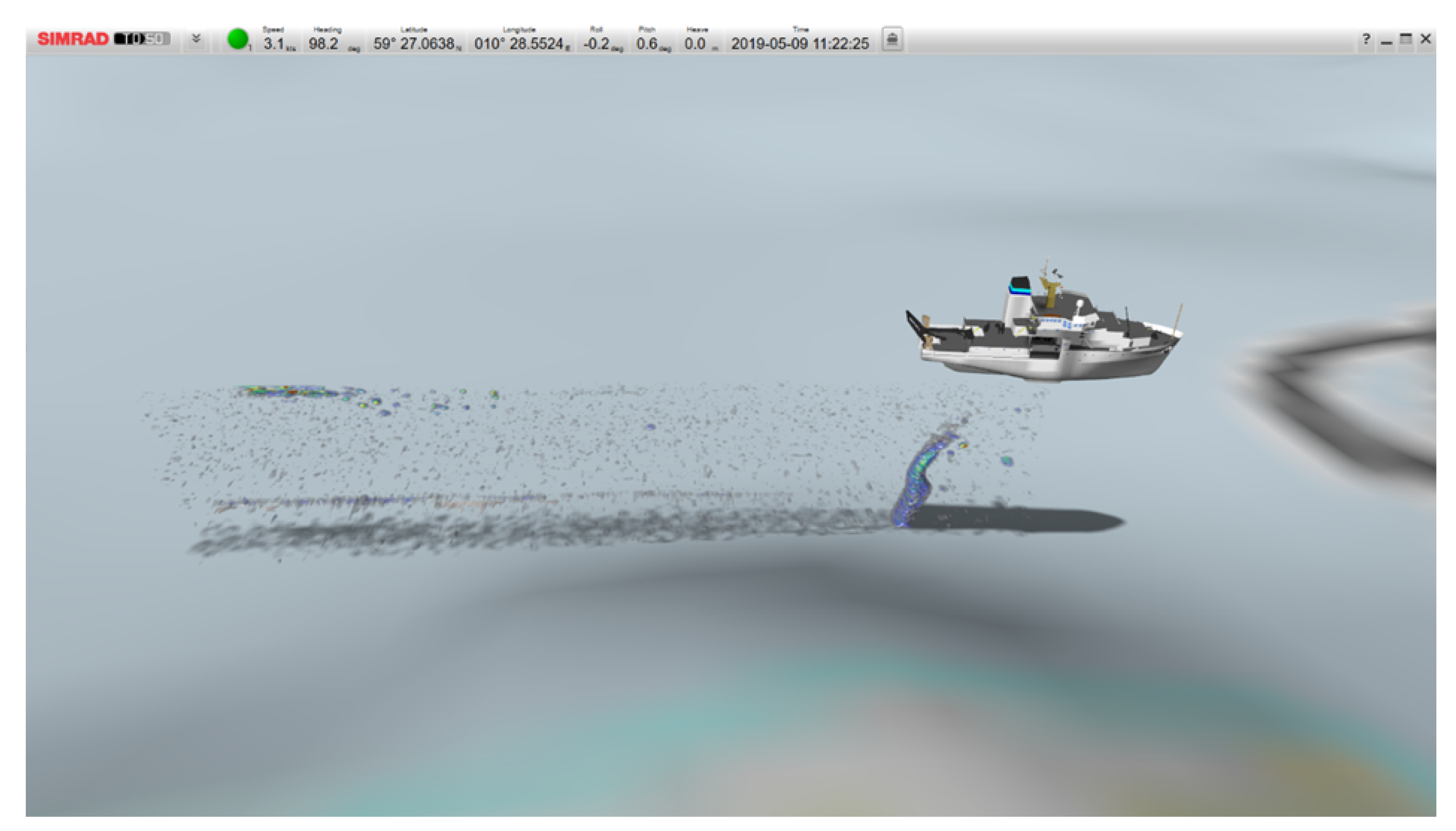
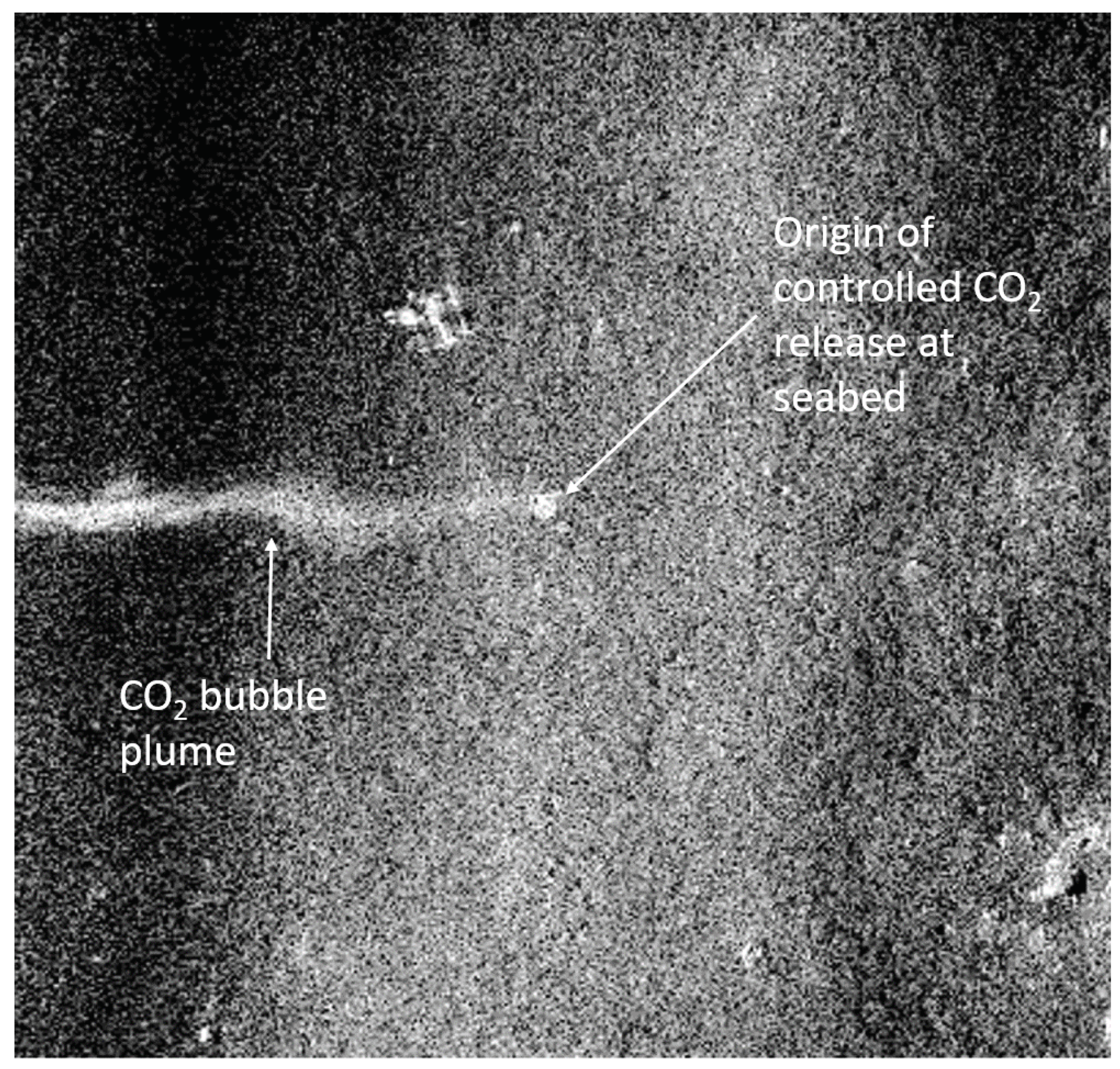
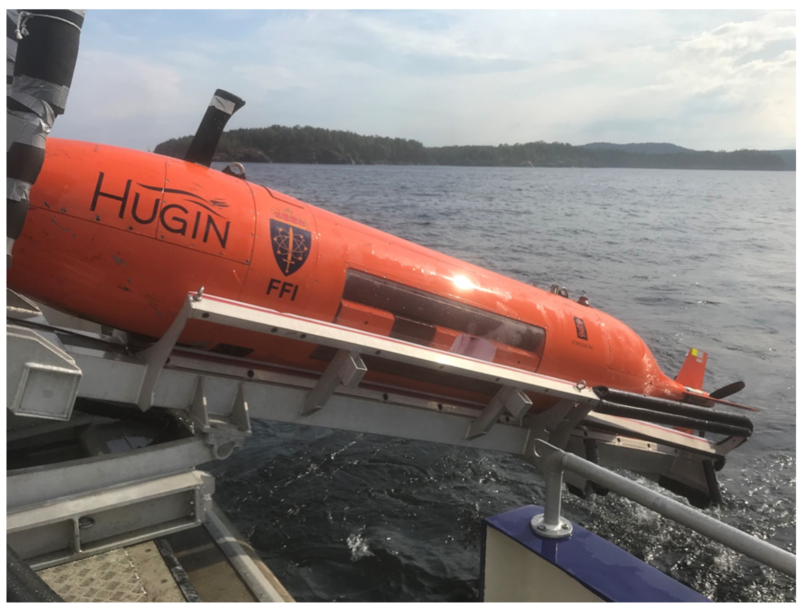
• Selecting and combining sensors and platforms to detect, attribute and quantify potential leakage, and conversely, to document the lack thereof. This includes sensors capable of detecting and characterizing different aspects of potential leakage, such as bubble seeps, chemical changes in the water column, and features in the marine environment, such as pockmarks, bacterial mats or gas-saturated sediments. Platforms on which these sensors may be mounted include surface vessels/ships, AUVs, gliders, and stationary templates. A strategy for how to use and combine these technologies should ensure adequate and practically/economically feasible monitoring.
• Extracting key information. Depending on the monitoring strategy, the amount of data quickly becomes unmanageable and human interpretation impractical. Dedicated data analysis is required to extract key information from significant and diverse data sets. Machine learning may play a significant role in differentiating between natural variability and potential leakage.

Regulations for marine monitoring of offshore CCS are set out in the CCS directive [2] from 2009, and were revised in 2015. These regulations define a minimum of required marine monitoring, but they do not specify the details of how to establish a meaningful monitoring program. While member states are required to report to the European Commission on the implementation of the directive every four years, there is no provision for continuous updates of the CCS directive. Consequently, the monitoring requirements may not be sufficiently up to date and reflective of recent technological advancements.

In this review, we condense recommendations and knowledge about marine GCS monitoring obtained through several research projects and many years of commercial CCS operations. Recommended strategies for marine monitoring are generally well aligned between the research projects considered here (ECO2, QICS, STEMM-CCS, ACT4storgae, ETI-MMV), and key components of these are described in Section 2. It is worth noting that these projects have had significant industry participation, indicating that the recommendations are aligned with industry perspectives.

In Section 3, we provide an overview of the most relevant technologies for marine GCS monitoring, including which sensors are applicable to different monitoring tasks, and the variety of platforms (ships, autonomous underwater vehicles (AUVs), stationary monitoring stations) that these sensors may be mounted on, depending on monitoring needs. Finally, we identify knowledge gaps and indicate future directions of research in Section 4.

2. Strategies for Marine GCS Monitoring

A number of research projects have addressed strategies for marine GCS monitoring, providing guidance about how to monitor the marine environment in sufficient detail without prohibitive costs [4,7,11,12,13,14,15]. Considering that the probability of leakage from a well-planned CO₂ storage site is considered low [5,6], it is generally not necessary or economically sound to monitor the entire region in detail over an extended period of time. A meaningful strategy combines sparse mapping of regions where there are no identified risk zones, with more resource-intensive monitoring either near risk structures, such as infrastructure (wells) and natural migration paths (faults, channels, pockmarks), or triggered by observations, such as deviations between models and measurements. In this section, we condense the recommendations provided by five major research projects carried out between 2011 and 2019; QICS, ECO2, ETI-MMV, ACT4storage, and STEMM-CCS. While there are slight variations in the viewpoints presented through these projects, the high-level recommendations for marine monitoring strategies are very much aligned.

2.1. Cite Characterization—Understanding the Baseline

All evaluated projects highlight the importance of obtaining a strong baseline, sometimes also referred to as site characterization, prior to injection of CO₂. The motivation for cite characterization is to obtain an understanding of the marine environment in the area, including natural variability. A strong understanding of the marine environment and its variability, both spatially and over considerable time scales, makes it easier to identify anomalies potentially related to CO₂ leakage. Further, these insights can prevent falsely attributing naturally occurring events to the ongoing CCS project. While there is agreement about the benefits of obtaining a strong baseline, there are different viewpoints related to the required level of detail as well as the timeline for building the baseline. Hypothetical leakage scenarios span from integrity issues with the injection well resulting in immediate leakage, to gradual migration of CO₂ from the reservoir along a geological risk structure, which would take several years to reach the marine environment [16]. Thus, the characteristics of a leak, including the delay from injection until an anomaly may be detectable in the marine environment, is complex and related to the geological conditions in the area as well as the presence and state of the infrastructure. In [12], the authors provide an overview of monitoring methodologies and recommended spatial and temporal sampling criteria for a baseline study. The specific requirements for a baseline study are related to a site-specific risk assessment, including potential risk structures and associated hypothetical leakage scenarios.

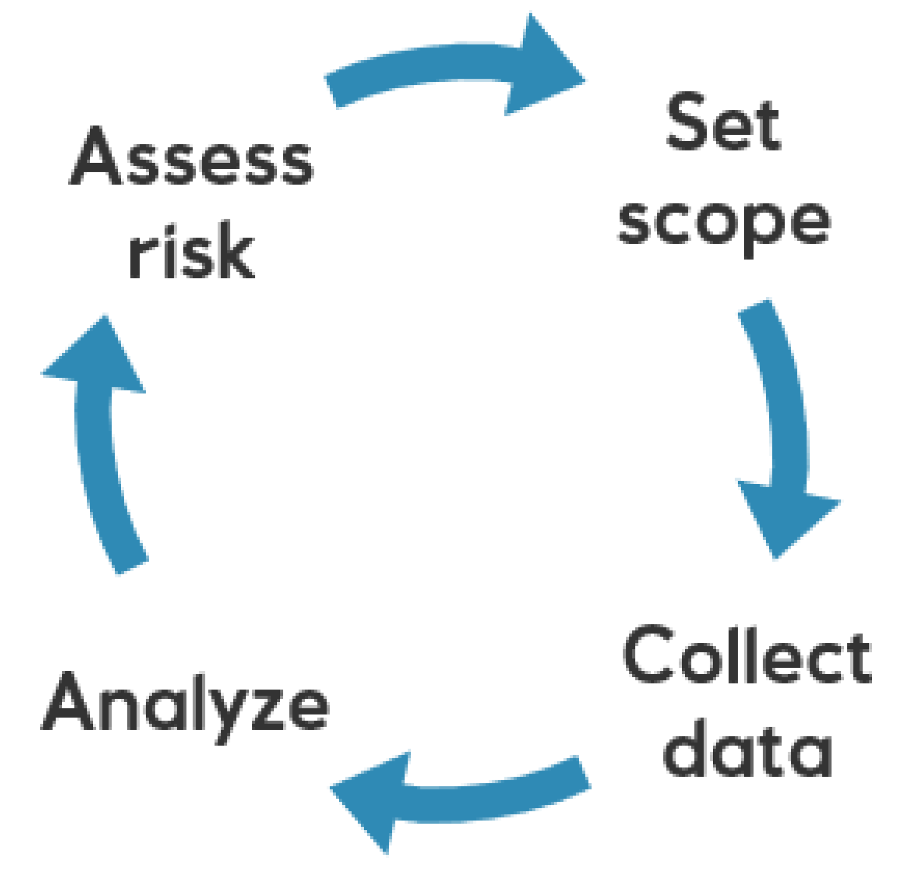
2.2. Using a Risk-Based Approach

A risk-based approach is recommended to focus monitoring efforts where they are most needed. Three-dimensional seismic data, either acquired as part of the site characterization of the reservoir or available from previous exploration activity, are used in the risk analysis to identify potential natural risk features, such as chimney structures, faults intersecting the reservoir, and subsurface channels. Marine surveys may reveal indications of past or ongoing fluid flow at the seabed, such as pockmarks, bacterial mats, or gas seepage. Additional risk structures include infrastructure—in particular, legacy wells. An initial risk analysis is intended to identify these structures and evaluate the risk of leakage as well as estimate the resulting environmental impact. Subsurface and ocean models combined with simulations of potential leakage scenarios may be used to predict the environmental impact related to identified risk structures. The risk analysis is a cyclic process, with new knowledge continuously being taken into account to adjust the current risk level. At CCS sites with no significant risk structures, resource-intensive marine monitoring may be recommended only as part of a contingency plan, to be triggered if an anomaly is encountered in, for example, seismic time-lapse data or in-well pressure measurements. In cases where risk structures are present, dedicated marine monitoring may be necessary to verify that there is no leakage through these structures, and to ensure that potential leakage is promptly detected such that corrective actions may be taken. The bowtie method, based on the barrier approach to risk management [11,17], provides a framework for a systematic risk assessment, including identifying risks and proposing proportional monitoring efforts. Figure 1 illustrates a risk-based approach to marine GCS monitoring, where an initial monitoring scope is set based on available information and an initial risk assessment, and is continuously re-evaluated as new information becomes available.

2.3. A Site-Specific and Flexible Marine Monitoring Program

The marine monitoring program should be tailored to the specifics of the location and, in particular, related to a site-specific risk analysis. The monitoring program should also be designed to adapt to changes in the risk level, for example, initiated by anomalous measurements (increased risk level), or added confidence in storage containment (reduced risk level). Additional factors that may influence the optimal approach to marine monitoring include the available infrastructure, water depth and ocean currents, and characteristics of the overburden. If shallow risk structures are identified in the overburden, a marine monitoring program can be designed to detect potential precursors of leakage based on expected changes in sediment or seawater geochemistry. The number of wells and the state that they are in will affect the need for detailed and potentially continuous monitoring. Finally, relevant data already available from the site, such as previous seismic surveys, bathymetry maps, and sediment and water samples, should be used as part of the site characterization process.

3. Overview of Marine Monitoring Technologies

Because of the complexity of the marine environment and the range of processes potentially indicative of CO₂ leakage (gas bubbles in the water or sediments, excess levels of dissolved CO₂ in the water column and related geochemical disturbances, excess fluid flow, etc), there are a variety of sensor technologies that are applicable to marine GCS monitoring. Generally, a combination of several sensor technologies is required to adequately describe the marine environment and detect or document the lack of potential leak-related anomalies. The two most widely used classes of technologies for marine GCS monitoring are acoustic sensors (aimed at detecting bubbles in the water column, mapping the seabed, and providing quantitative estimates of bubble emissions), and chemical sensors (aimed at detecting and characterizing chemical anomalies in sea water, and establishing baseline chemical seawater conditions). These may be complemented by additional sensors, such as CTDs, ocean current meters, and optical and turbidity sensors, for more complete mapping of the ocean environment.

Selecting an appropriate combination of technologies to be used in a site-specific monitoring campaign is non-trivial. A recurring challenge is how to achieve the required area coverage with satisfactory spatial and temporal resolution, and without prohibitive costs. On the one hand, in many cases, the large area to be covered suggests the use of survey vessels or autonomous underwater vehicles (AUVs) to achieve the required area coverage rates. On the other hand, the spatial footprint as well as the temporal duration of leakage events is expected to be limited (in the order of tens of meters and hours to days in duration [10]), requiring more focused and sometimes long-term monitoring to capture these events.

Table 1. Overview of relevant marine GCS monitoring objectives, and sensor technologies and platforms with corresponding capabilities.

Monitoring Objective	Sensor Technology	Platform
Detect bubbles in the water column (single bubbles, seeps or plumes)	MBES, SBES, sidescan sonar, SAS	Survey vessel, AUV, stationary template
Identify seabed features related to fluid flow	MBES, SAS, sidescan sonar	Vessel, AUV
Identify sub-seabed features including shallow gas accumulation	SBP	Survey vessel, AUV
Quantify gas-phase CO2 emission from seabed	SBES, direct measurement	Survey vessel, stationary template, AUV
Identify anomalous chemical signature in water masses	pCO2, pO2, pH, CTD, other chemical	Stationary template, glider, AUV, survey vessel
Quantify amount of excess CO2 in the water masses	pCO2, pO2, pH, CTD, other chemical	Stationary template, glider, AUV, survey vessel

summarizes different potential monitoring objectives and corresponding sensors and platforms that may be used to reach these objectives. These technologies and their capabilities for marine GCS monitoring are elaborated on in the remainder of this section.

3.1. Acoustic Sensors

Active acoustic sensors (sonars and echo sounders) rely on transmitting sound and using the reflected signal to detect the presence of bubbles in water or sediments, or to map the seabed [18]. Active acoustic sensors are particularly useful for detecting bubbles at a distance (tens to hundreds of meters for modest bubble seepage) because gas-filled bubbles in water are excellent acoustic targets. The detection range depends on the properties of the leak, such as the leak rate and bubble size distribution, as well as the type of acoustic sensor and its properties. Relevant acoustic sensor technologies are described below, and examples of documented system-specific seep detection ranges are provided. While it is common to mount active acoustic sensors on surface vessels or AUVs, they can also be mounted on a stationary platform for long-term monitoring of a region of interest, such as a well or above a geological risk structure [15,19,20,21].

Marine acoustics is a well-explored and mature field, and there are many active acoustic sensors available on the market, ranging from low-frequency sensors with long range and, in some cases, sediment penetration capabilities [22,23], to high-frequency, high-resolution systems suitable for detailed monitoring at close range [24]. Relevant active acoustic sensors for marine GCS monitoring include single- and split-beam echo sounders (SBES), multibeam echo sounders (MBES), imaging and fish-finding sonars, side scan sonars, and synthetic aperture sonar (SAS). Selecting the appropriate acoustic sensor depends on the monitoring task, in particular, the required range and area coverage rate, the required sensitivity (i.e., detecting single bubbles or larger emissions), and whether or not acoustic quantification is a requirement. For seabed mapping purposes, the required image quality and resolution need to be considered.

Side scan sonars are often mounted on AUVs and used to map the seabed. In the context of marine GCS monitoring, side scan sonars are highly useful tools because they can cover a large area efficiently and detect both bubble seepage in the water column and map the seabed, including features indicative of fluid flow and marine habitats [25,26,27,28]. The imaging and bubble-detection range of side scan sonars is system- and site-dependent, with typical ranges in the order of 50 to 200 m. Several publications demonstrate the use of an AUV-mounted side scan sonar to detect bubble seepage of CO₂ and CH₄ at the seabed [26,27]. While there are few studies that quantitatively investigate the detection range and sensitivity of side scan sonars in the context of bubble seepage, a few examples have been published. In [27], a modest amount of CH₄ escaping from an abandoned well is automatically detected at a distance of 110 m range using a side scan sonar operating at a center frequency of 100 kHz. In [26] the authors present an experiment using a dual frequency side scan sonar operating at 300 kHz and 600 kHz. Here, the observed detection limits are in the order of 10–20 m at a leak rate of 1 liter/minute of CO₂.

SAS systems are based on hardware similar to a side scan sonar but were developed to achieve dramatically improved image resolution independent of range. In recent years, SAS has matured into a powerful tool, providing detailed seabed imagery and bathymetry as well as the ability to detect small-scale seabed features, including bacterial mats [29], in addition to bubble seepage. Example images (Figure 2) obtained during the ACT4storage controlled release experiment [30] show a 1.33 liter/min release of CO₂ bubbles imaged using the HISAS 1030 system mounted on the HUGIN AUV at a ground range (distance as measured along the seabed) of 60 m. Note that the aim of this experiment was not to demonstrate the detection range of the sonar and, thus, larger distances were not evaluated. Both for side scan sonars and SAS systems, the imaging geometry as well as the operating frequency of the system should be considered. Detection ranges and area coverage rates may be increased by utilizing low to medium frequency systems, and allowing the AUV to travel at a significant height above the seabed [15].

Echo sounders, both single- and multibeam, are traditionally mounted on the hull of a survey vessel and directed downward to map the water column and seabed. As the name suggests, an SBES emits a single acoustic beam and records the intensity of the echo reflected from the seabed and objects or particles in the water column. Single bubbles, bubble trains and bubble plumes are recognized based on their characteristic shape in the echogram [31,32]. Split-beam echo sounders make use of four separate quadrants on reception, which makes it possible to position a target more accurately. More importantly in this context, state-of-the-art split beam echo sounders may be absolutely calibrated, enabling acoustic quantification of bubble seepage [33,34,35]. MBES systems transmit multiple beams simultaneously, providing significant area coverage, with swath widths up to 140°. As such, vessel-mounted MBES provide a cost-efficient means of mapping a large region of the seabed, while simultaneously detecting the presence of gas seeps in the water column. In [30], small CO₂ bubble releases down to 0.1 liter/minute are consistently detected and visible in the echogram from an EK80 SBES and several MBES systems operating at different frequencies (EM2040, EM712, ME70 and SN90). Figure 3 shows an example image obtained using the Simrad ME70 MBES during the controlled release of 1.3 liters/minute of pure gaseous CO₂.

A sub bottom profiler (SBP), sometimes also referred to as a shallow seismic sensor, is designed to penetrate the upper few meters of sediments (approximately 5–100 m, depending on sediment properties). These sensors either operate at low frequencies, or make use of non-linear propagation to generate a low-frequency pulse that is able to penetrate the seabed. In the context of GCS, SBPs are highly useful because they can reveal shallow risk structures, including shallow gas accumulations and potential migration pathways such as salt diapers, pockmarks and faults [36,37]. These shallow features in the upper sediments are not easily captured using traditional seismics. Combining seismic imagery of the reservoir and deep geological layers with SBP data of the shallow sediments and acoustic mapping of the seabed and water column makes it possible to capture and interpret features ranging from the reservoir to the sea surface.

Passive acoustic sensors, or hydrophones, can be used to detect the presence of bubbles based on their acoustic emissions [18]. Several studies demonstrate the capability to quantify bubble seepage using passive acoustic sensors [38,39], although further studies are encouraged to investigate the accuracy of these estimates. The detection range depends on the background noise level, leak rate, and sensitivity of the sensor. Hydrophones have low power consumption, making them ideal for long-term deployment on stationary monitoring platforms in the vicinity of a risk structure, or on a moving vehicle, such as a glider with limited battery capacity.

3.2. Chemical and Oceanographic Sensors

While acoustic sensors are able to detect the presence of bubble seepage and related seabed features, chemical sensors are required to monitor the chemical composition of seawater, and to detect anomalies potentially related to CO₂ leakage. In the event of CO₂ escaping the reservoir and reaching the marine environment, changes in the carbonate chemistry of seawater may be detected as a spatially limited water mass with an anomalously high CO₂ concentration and, as a result, reduced pH. The chemical and spatial characteristics of such plumes may vary depending on the leak scenario and site-specific parameters. Depending on the properties of the upper sediments and overburden, a plume with additional characteristic properties, such as high salt content or the presence of characteristic heavy metals, may be an early indication of a pressure buildup prior to CO₂ leakage [13]. Robust chemical monitoring requires careful planning since the area to be covered is large, while the chemical footprint of a leak-related plume is expected to be small [40]. The trade-off in spatio-temporal resolution and area coverage needs to be carefully considered. While moving vehicles such as an AUV or a glider can provide an overview of an area at limited spatio-temporal resolution, fixed seabed installations can be used for continuous monitoring of a focus area at high temporal resolution. The ability to chemically detect a plume using a moving platform sets demands to the sensitivity of the sensor (i.e., the ability to detect a diluted plume over the background concentration), and is further limited by the dynamic response time of the sensor.

Relevant chemical sensors for marine GCS monitoring include CO₂, O₂, and pH sensors. Sensors for detecting metal contents may also be useful in order to detect pore fluids emanating from the seabed as a precursor to CO₂ emissions. Similarly, salinity, temperature, turbidity, fluorescence and optical sensors may reveal deviations from normal conditions caused by a pressure buildup in the reservoir or overburden, forcing shallow pore fluids and particles into the marine environment. CH₄ (methane) sensors are relevant in cases where one needs to differentiate between CO₂ and CH₄, for instance, to ensure that detected bubble plumes are related to shallow CH₄ emissions and cannot be attributed to an ongoing CO₂ storage project. Because CO₂ is considerably more soluble than CH₄ in seawater, CO₂ bubbles dissolve faster and do not reach the same height in the water column as a CH₄ bubble plume with a comparable bubble size distribution. However, CO₂ bubbles have been observed to rise higher than previously expected, potentially due to the gas exchange allowing other, less-soluble gases to enter the bubble as the CO₂ dissolves into the surrounding water [41]. Thus, chemical verification is recommended in addition to visual inspection of acoustic echograms to unambiguously differentiate between the two substances. In addition, project-specific knowledge, such as the use of a chemical tracer in the injected CO₂ or site-specific chemical composition of the overburden, may merit the use of other chemical sensors.

Chemical sensors are point sensors, and need to be inside the chemical plume in order to detect it. Therefore, the detection range of chemical sensors is affected by the properties of the plume and the effects of ocean currents. Since a CO₂ plume is quickly diluted in seawater, sensors need to be located within a few tens of meters of the leak origin to detect it. Experimental and modeling results indicate that the detection distance depends greatly on the emission rate as well as on ocean currents [10,42]. In [10], the authors have modeled a set of hypothetical leak scenarios and suggest similar detection ranges. For a 1 T CO₂/year leak rate and ocean conditions representative of the North Sea, the authors estimate a chemical detection range of 60 m. At the same time, the impact radius (i.e., distance at which benthic habitats are temporarily affected by the leak) is estimated to be significantly smaller at 15 m. An understanding of the plume dynamics, including its spatial and temporal evolution, is important when planning either the location of stationary monitoring stations or the travel path of an AUV.

Currently available CO₂ and CH₄ sensors use a membrane through which the seawater diffuses before measurement. The diffusion process takes some time, which is reflected in the sensor response time. This becomes a challenge when the sensors are placed on moving platforms because the sensors may not have time to react properly to spatially limited plumes. When possible, faster responding sensors, such as pH, temperature and salinity, may be useful complementary sensors that can improve plume detectability. In particular, since pH is closely linked to CO₂ (an increase in the CO₂ content causes a reduction in pH), a pH sensor may be used as a proxy for a CO₂ sensor. This requires selection of a pH sensor with high sensitivity, in the order of 0.01, to detect the expected pH change induced by a CO₂ plume [10,42,43].

The water column, seabed and atmosphere are all part of an open system that is affected by a vast number of natural processes. Monitoring the water column therefore poses the considerable challenge of separating natural variability from anomalies related to unintended leakage from the reservoir. A strong understanding of the variability and heterogeneity of the ocean environment and, in particular, the carbonate chemistry is required to identify anomalies potentially related to a leak event without falsely attributing natural variability to the ongoing storage project. It is often necessary to evaluate several parameters together in order to identify key relationships that are expected both as part of the natural marine variability, and during a potential leakage event. For example, the coherence between CO₂ and O₂ is identified as a key chemical marker to differentiate between a leakage event and natural variability [42,44,45]. The authors in [46] use a stoichiometric method (C${}_{seep}$) to differentiate between potential CO₂ leakage and natural variability. Yet another approach to differentiating between natural variability and potential leakage is described in [14], where the authors use a coupled hydrodynamic–biogeochemical model to characterize the carbonate chemistry and recommend anomaly detection criteria.

3.3. Emerging Technologies

Significant technological progress has been made over the past years, and several promising technologies have been demonstrated but are not yet commercially available. The lab on a chip (LOC) technology was developed to enable standard wet laboratory procedures in situ, using a miniaturized chip [47,48], thereby significantly reducing the intensive post-analysis workload. While an ISFET pH sensor based on the LOC technology is commercially available, additional LOC sensors to measure the total alcalinity (TA) and nutrients were demonstrated during a controlled release experiment in the North Sea carried out as part of the STEMM-CCS project [7]. The eddy covariance method has been used for some time to detect and quantify CO₂ emissions to the atmosphere [49,50]. The method was recently demonstrated to monitor CO₂ escaping the seabed during a controlled CO₂ release experiment [51]. The eddy covariance method requires that the monitoring equipment is placed in the direct vicinity of the source, making it a promising technology for lthe ong-term monitoring and quantification of a known leak. Fiber optic technology is rapidly advancing and seeing new areas of application. In the context of marine GCS monitoring, fiber optic sensing may provide a cost-effective means of monitoring subsidence and upheaval potentially related to the geological injection of CO₂.

3.4. Sensor Platforms

Monitoring sensors can be placed on different platforms, depending on the monitoring requirements, in particular, the size of the area to be covered, the level of detail required, and the time frame for monitoring. Relevant platforms include surface vessels, AUVs, gliders (also a type of AUV), and stationary monitoring solutions.

3.4.1. Surface Vessels

A surface vessel, such as a survey ship or a seismic acquisition vessel, can efficiently survey a large area. A cost-efficient solution can be to combine the marine monitoring survey with other planned activities using these vessels, such as seismic acquisition or research expeditions. A vessel-mounted MBES provides efficient mapping of the water column (to document bubble seepage) and simultaneous seabed bathymetry mapping. If quantitative estimates of bubble flux from detected seeps are required, a calibrated echo sounder can be mounted on the same vessel. Measurements from the water column and seafloor can be complemented by SBP data revealing shallow structures in the upper sediments. Mapping the upper sedimentary layer can be helpful in data interpretation, potentially indicating whether a seabed feature is non-problematic for the storage project, or whether it can be related to a deeper risk structure. MBES and SBPs operate at distinctly different frequencies and can normally be operated simultaneously without acoustic interference affecting the data quality. These remote sensing techniques may be complemented by water and sediment samples collected at strategic locations. A surface vessel may also carry supplementary equipment, such as a towfish, with suitable acoustic and/or chemical/oceanographic sensors aimed at mapping deeper sections of the water column or seabed. The optimal vessel speed and line spacing is affected by the water depth and the area coverage of the sensors used. A conservative estimate of the area coverage rate in 100 m water depth and when using a MBES and an SBF is in the order of 4–6 km²/h [15].

3.4.2. Autonomous Underwater Vehicles

While ship-based surveys are highly efficient for mapping large areas, AUVs have the additional advantage of traveling near the seabed and can therefore provide detailed information about the deep ocean layers and document the seabed on a finer scale. Their potentially significant sensor payload (subject to vehicle-specific limitations) enables AUVs to sample many parameters simultaneously for a complete chemical, oceanographic and acoustic survey. The AUV sensor payload can be adjusted according to monitoring needs, for example, detailed mapping of the seabed using side scan or synthetic aperture sonar (SAS) to document pockmarks, bacterial mats and bubble seeps, while simultaneously measuring the level of dissolved CO₂, pH, O₂, salinity, temperature and turbidity. Depending on the capacity of the vehicle, the AUV may also carry a MBES and a sub-bottom profiler. A high-definition subsea camera can be used to document special areas of interest. State-of-the-art AUVs today follow a pre-programmed data acquisition path. A common data acquisition path is a lawn-mower pattern at a single depth, but this can be tailored to the monitoring needs. A wide range of AUVs are currently available on the market, ranging from small, low-power vehicles with a limited sensor payload but extended operation times, to larger and more power-demanding AUVs capable of carrying a significant sensor payload, including state-of-the art imaging sonars for detailed seabed mapping. Typical operational times are in the order of days. Area coverage rates are vehicle-, payload-, and location-specific. For the HUGIN AUV (Figure 4) equipped with chemical sensors and a SAS system, area coverage rates are estimated to be in the order of 2 km²/h. AUV-related research efforts are currently directed toward improved vehicle autonomy, including the ability for the vehicle to actively adapt to its environment [52,53] and endurance [54,55], as well as on solutions with resident AUVs able to re-charge their batteries using subsea docking stations [56] or wireless charging systems [57].

3.4.3. Gliders

Gliders are a specialized type of AUV, described separately here for clarity. Traditional gliders do not use a propeller but a combination of hydrofoils and buoyancy control to maneuver in a zig-zag pattern between two depths in the water column. This low-power solution allows for long-term deployment of up to several months depending on sensor payload and battery capacity. In the context of marine monitoring for GCS, these vehicles are particularly well suited for gathering oceanographic data from vast ocean areas. Information about long-term temporal and spatial variability in ocean geochemistry enables more robust differentiation between natural variability and potential anomalies, and is also valuable input to oceanographic models. Gliders are generally optimized for long endurance, and therefore carry a limited sensor payload compared to AUVs. Typical sensor payloads include CTDs, salinity, and turbidity sensors. Chemical sensors have also been demonstrated, including pH, CO₂, and CH4. As mentioned above, the relatively long response times of currently available CO₂ and CH₄ sensors make them less suited for deployment on a moving platform. This is particularly problematic for a glider that moves up and down in the water column because of the significant naturally occurring vertical variability in these parameters. In recent years, new glider platforms have become available on the market, including surface gliders and hybrid gliders. The latter use a propeller to mimic AUV-maneuverability for short periods of time. Glider sensor payloads are also in rapid development, with recent advancements including a scientific echo sounder [58].

3.4.4. Stationary Monitoring Solutions

Stationary monitoring solutions can take many forms, including seabed templates deployed for long periods of time (months or years), temporarily deployed landers, or remotely operated vehicles (ROVs) maintaining a fixed position for some period of time. Stationary monitoring solutions are particularly relevant near identified risk structures, but may also be used to collect baseline data at strategic locations or prior to CO₂ injection. Which sensors to install will depend on the available infrastructure for power supply and data management, and on the monitoring requirements. Typical low-power sensors include chemical and oceanographic sensors as well as hydrophones, while active acoustic sensors (sonars and echo sounders) are more power demanding. Stand-alone solutions, including echo sounders deployed for several months, are commercially available.

For chemical and oceanographic monitoring, remaining at a fixed position over time and acquiring data at a high sample rate increases the ability to detect small or diluted chemical plumes. Because most chemical and oceanographic parameters have larger variability in the vertical direction than in the horizontal direction, maintaining a fixed vertical position over time results in less noise in these measurements.

3.5. The Role of Modeling

The lack of sufficient observational data both on a temporal and spatial scale implies that models have a significant role to play in the context of marine GCS monitoring [14,59]. While the marine environment has been studied for decades, it remains poorly described if we consider only the available observational data. However, a range of marine system models have been developed to describe both physical flow (ocean currents and tidal effects) and biogeochemical systems, including carbonate chemistry. Specialist models may be used to describe leak-related features, such as bubble plume dynamics [41,60]. For CCS, marine models contribute to the baseline by providing complementary information about natural variability where observational data are lacking or incomplete. Further, the ecological impact of hypothetical leakage may be estimated based on numerical leakage simulations. Finally, the predicted footprint, or spatial and temporal extent of the leakage signal, has direct implications for the choice of monitoring strategy as well as sensor and platform configuration. Sensors must have sufficient sensitivity and be placed at an appropriate distance to detect an anomaly related to relevant leakage scenarios as identified during the risk assessment. Modeled predictions of leakage footprint may also be used to optimize the placement of stationary monitoring platforms as well as the travel path of an AUV [59,61].

4. Knowledge Gaps and Future Research Directions

Marine GCS monitoring has received significant attention over the past years, and there are now mature technologies and methodologies available on the market to allow adequate monitoring. High-resolution models and simulations of hypothetical leakage scenarios provide important knowledge where observational data are scarce. Strategies for cost-efficient monitoring have been developed and are generally agreed upon within the scientific community and supported by commercial operators. The remaining technological challenges can be categorized into sensor development, data management, and enhanced autonomy reducing the need for costly human involvement.

Sensor development related to emerging technologies as indicated in Section 3.3 is expected, as is further optimization of available technologies to improve their functionality related to marine GCS monitoring. Efforts are currently being directed toward reducing the response time of available CO₂ sensors, making them more relevant for deployment on AUVs and gliders.

AUVs have the potential to play a key role in marine GCS monitoring because of their ability to cover large areas and to carry a range of chemical, oceanographic and acoustic sensors. Currently, these vehicles have limited decision autonomy and therefore follow a pre-defined travel path. “Truly autonomous” AUVs capable of acting intelligently based on their surroundings as measured by sensor measurements in real time are technologically within reach, and would significantly improve the cost-efficiency of these vehicles. This requires development related to data analysis, in particular, translating raw sensor data into high-level information based on which the vehicle can make an intelligent decision in real time. It also requires development related to AUV travel path optimization and real-time adaptation.

Finally, frameworks for managing the large amounts of data produced by different sensors acquiring high-resolution data over time need to be developed or tailored to the needs of the monitoring program. Streamlined solutions for data communication and information sharing between the different components of a monitoring program would further increase the efficiency of marine GCS monitoring. Big data analysis and machine learning techniques are expected to play a role in extracting key information efficiently from these significant data sets.

References

1. Gale, J.; Abanades, J.; Bachu, S.; Jenkins, C. Special issue commemorating the 10th year anniversary of the publication of the intergovernmental panel on climate change special report on CO2 capture and storage. Int. J. Greenh. Gas Control 2015, 40, 1–5. [Google Scholar] [CrossRef]
2. Metz, B.; Davidson, O.; de Coninck, H.; Loos, M.; Meyer, L. IPCC Special Report on Carbon Dioxide Capture and Storage. Prepared by Working Group III of the Intergovernmental Panel on Climate Change; Technical Report; Cambridge University Press: Cambridge, UK; New York, NY, USA, 2005. [Google Scholar]
3. Ringrose, P.S.; Meckel, T. Maturing global CO2 storage resources on offshore continental margins to achieve 2DS emissions reductions. Sci. Rep. 2019, 9, 17944. [Google Scholar] [CrossRef]
4. Furre, A.K.; Eiken, O.; Alnes, H.; Vevatne, J.N.; Kiær, A.F. 20 Years of Monitoring CO2-injection at Sleipner. Energy Procedia 2017, 114, 3916–3926. [Google Scholar] [CrossRef]
5. Global CCS Institute. The Global Status of CCS: 2019; Technical Report; Global CCS Institute: Canberra, Australia, 2019. [Google Scholar]
6. Alcalde, J.; Flude, S.; Wilkinson, M.; Johnson, G.; Edlmann, K.; Bond, C.; Scott, V.; Gilfillan, S.; Ogaya, X.; Haszeldine, S. Estimating geological CO2 storage security to deliver on climate mitigation. Nat. Commun. 2018, 9, 2201. [Google Scholar] [CrossRef]
7. Dean, M.; Blackford, J.; Connelly, D.; Hines, R. Insights and guidance for offshore CO2 storage monitoring based on the QICS, ETI MMV, and STEMM-CCS projects. Int. J. Greenh. Gas Control 2020, 100, 103120. [Google Scholar] [CrossRef]
8. Tanaka, Y.; Sawada, Y.; Tanase, D.; Tanaka, J.; Shiomi, S.; Kasukawa, T. Tomakomai CCS Demonstration Project of Japan, CO2 Injection in Process. Energy Procedia 2017, 114, 5836–5846. [Google Scholar] [CrossRef]
9. Jenkins, C.; Chadwick, A.; Hovorka, S.D. The state of the art in monitoring and verification—Ten years on. Int. J. Greenh. Gas Control 2015, 40, 312–349. [Google Scholar] [CrossRef] [Green Version]
10. Blackford, J.; Alendal, G.; Avlesen, H.; Brereton, A.; Cazenave, P.W.; Chen, B.; Dewar, M.; Holt, J.; Phelps, J. Impact and detectability of hypothetical CCS offshore seep scenarios as an aid to storage assurance and risk assessment. Int. J. Greenh. Gas Control 2020, 95, 102949. [Google Scholar] [CrossRef]
11. Dean, M.; Tucker, O. A risk-based framework for Measurement, Monitoring and Verification (MMV) of the Goldeneye storage complex for the Peterhead CCS project, UK. Int. J. Greenh. Gas Control 2017, 61, 1–15. [Google Scholar] [CrossRef]
12. Blackford, J.; Bull, J.M.; Cevatoglu, M.; Connelly, D.; Hauton, C.; James, R.H.; Lichtschlag, A.; Stahl, H.; Widdicombe, S.; Wright, I.C. Marine baseline and monitoring strategies for carbon dioxide capture and storage (CCS). Int. J. Greenh. Gas Control 2015, 38, 221–229. [Google Scholar] [CrossRef] [Green Version]
13. ECO2. ECO2 Final Publishable Summary Report; Technical Report; Available online: https://www.eco2-project.eu/ (accessed on 27 August 2021).
14. Blackford, J.; Artioli, Y.; Clark, J.; de Mora, L. Monitoring of offshore geological carbon storage integrity: Implications of natural variability in the marine system and the assessment of anomaly detection criteria. Int. J. Greenh. Gas Control 2017, 64, 99–112. [Google Scholar] [CrossRef]
15. Blomberg, A.E.A.; Waarum, I.K.; Eek, E.; Totland, C.; Lorentzen, O. ACT4storage—Acoustic and Chemical Technologies for Environmental GCS Monitoring. D4—Recommended Guidelines Report; Technical Report; Norwegian Geotechnical Institute: Oslo, Norway, 2020. [Google Scholar]
16. Vinca, A.; Emmerling, J.; Tavoni, M. Bearing the Cost of Stored Carbon Leakage. Front. Energy Res. 2018, 6, 40. [Google Scholar] [CrossRef] [Green Version]
17. Reason, J. Human error: Models and management. BMJ 2000, 320, 768–770. [Google Scholar] [CrossRef] [PubMed] [Green Version]
18. Medwin, H.; Clay, C.S. Fundamentals of Acoustical Oceanography; Academic Press: Cambridge, MA, USA, 1988. [Google Scholar]
19. Marcon, Y.; Kopiske, E.; Leymann, T.; Spiesecke, U.; Vittori, V.; von Wahl, T.; Wintersteller, P.; Waldmann, C.; Bohrmann, G. A Rotary Sonar for Long-Term Acoustic Monitoring of Deep-Sea Gas Emissions. In Proceedings of the OCEANS 2019—Marseille, Marseille, France, 17–20 June 2019; pp. 1–8. [Google Scholar]
20. Kubilius, R.; Pedersen, G. Relative acoustic frequency response of induced methane, carbon dioxide and air gas bubble plumes, observed laterally. J. Acoust. Soc. Am. 2016, 140, 2902–2912. [Google Scholar] [CrossRef]
21. von Deimling, J.S.; Greinert, J.; Chapman, N.R.; Rabbel, W.; Linke, P. Acoustic imaging of natural gas seepage in the North Sea: Sensing bubbles controlled by variable currents. Limnol. Oceanogr. Methods 2010, 8, 155–171. [Google Scholar] [CrossRef]
22. Ergün, M.; Dondurur, D.; Çifçi, G. Acoustic evidence for shallow gas accumulations in the sediments of the Eastern Black Sea. Terra Nova 2002, 14, 313–320. [Google Scholar] [CrossRef]
23. Hovland, M. Large pockmarks, gas-charged sediments and possible clay diapirs in the Skagerrak. Mar. Pet. Geol. 1991, 8, 311–316. [Google Scholar] [CrossRef]
24. Waarum, I.K.; Sparrevik, P.; Kvistedal, Y.; Hayes, S.; Hale, S.; Cornelissen, G.; Eek, E. Innovative Methods for Methane Leakage Monitoring Near Oil and Gas Installations. In Proceedings of the OTC Offshore Technology Conference, Houston, TX, USA, 3 May 2016. [Google Scholar]
25. Blondel, P. The Handbook of Sidescan Sonar; Springer: Berlin/Heidelberg, Germany, 2009. [Google Scholar]
26. Uchimoto, K.; Nishimura, M.; Watanabe, Y.; Xue, Z. An experiment revealing the ability of a side-scan sonar to detect CO2 bubbles in shallow seas. Greenh. Gases Sci. Technol. 2020, 10, 591–603. [Google Scholar] [CrossRef]
27. Blomberg, A.E.A.; Sæbø, T.O.; Hansen, R.E.; Pedersen, R.B.; Austeng, A. Automatic Detection of Marine Gas Seeps Using an Interferometric Sidescan Sonar. IEEE J. Ocean. Eng. 2017, 42, 590–602. [Google Scholar] [CrossRef]
28. Lucieer, V. Object-oriented classification of sidescan sonar data for mapping benthic marine habitats. Int. J. Remote Sens. 2008, 29, 905–921. [Google Scholar] [CrossRef]
29. Pedersen, R.B.; Blomberg, A.; Landschulze, K.; Baumberger, T.; Økland, I.; Reigstad, L.; Gracias, N.; Mørkved, P.T.; Stensland, A.; Lilley, M.D.; et al. Discovery of 3 km long seafloor fracture system in the Central North Sea. Available online: https://ui.adsabs.harvard.edu/abs/2013AGUFMOS11E..03P/abstract (accessed on 27 August 2021).
30. Blomberg, A.E.A.; Waarum, I.K.; Eek, E.; Totland, C.; Pedersen, G.; Lorentzen, O.; Loranger, S. ACT4storage—Acoustic and Chemical Technologies for Environmental Monitoring of Geological Carbon Storage. D3—Nearshore Evaluation Report 2019; Technical Report; Norwegian Geotechnical Institute: Oslo, Norway, 2020. [Google Scholar]
31. Nikolovska, A.; Sahling, H.; Bohrmann, G. Hydroacoustic methodology for detection, localization, and quantification of gas bubbles rising from the seafloor at gas seeps from the eastern Black Sea. Geochem. Geophys. Geosyst. 2008, 9. [Google Scholar] [CrossRef]
32. Blomberg, A.E.A.; Weber, T.C.; Austeng, A. Improved Visualization of Hydroacoustic Plumes Using the Split-Beam Aperture Coherence. Sensors 2018, 18, 2033. [Google Scholar] [CrossRef] [PubMed] [Green Version]
33. Weber, T.C.; Mayer, L.; Jerram, K.; Beaudoin, J.; Rzhanov, Y.; Lovalvo, D. Acoustic estimates of methane gas flux from the seabed in a 6000 km2 region in the Northern Gulf of Mexico. Geochem. Geophys. Geosyst. 2014, 15, 1911–1925. [Google Scholar] [CrossRef] [Green Version]
34. Weidner, E.; Weber, T.; Mayer, L.; Jakobsson, M.; Chernykh, D.; Semiletov, I. A wideband acoustic method for direct assessment of bubble-mediated methane flux. Cont. Shelf Res. 2019, 173, 104–115. [Google Scholar] [CrossRef] [Green Version]
35. Weber, T.C.; De Robertis, A.; Greenaway, S.F.; Smith, S.; Mayer, L.; Rice, G. Estimating oil concentration and flow rate with calibrated vessel-mounted acoustic echo sounders. Proc. Natl. Acad. Sci. USA 2012, 109, 20240–20245. [Google Scholar] [CrossRef] [PubMed] [Green Version]
36. Hempel, P.; Spieß, V.; Schreiber, R. Expulsion of Shallow Gas in the Skagerrak—Evidence from Sub-bottom Profiling, Seismic, Hydroacoustical and Geochemical Data. Estuar. Coast. Shelf Sci. 1994, 38, 583–601. [Google Scholar] [CrossRef]
37. Limonov, A.; van Weering, T.; Kenyon, N.; Ivanov, M.; Meisner, L. Seabed morphology and gas venting in the Black Sea mudvolcano area: Observations with the MAK-1 deep-tow sidescan sonar and bottom profiler. Mar. Geol. 1997, 137, 121–136. [Google Scholar] [CrossRef]
38. Bergès, B.J.; Leighton, T.G.; White, P.R. Passive acoustic quantification of gas fluxes during controlled gas release experiments. Int. J. Greenh. Gas Control 2015, 38, 64–79. [Google Scholar] [CrossRef] [Green Version]
39. Li, J.; White, P.R.; Roche, B.; Bull, J.M.; Leighton, T.G.; Davis, J.W.; Fone, J.W. Acoustic and optical determination of bubble size distributions—Quantification of seabed gas emissions. Int. J. Greenh. Gas Control 2021, 108, 103313. [Google Scholar] [CrossRef]
40. Vielstädte, L.; Linke, P.; Schmidt, M.; Sommer, S.; Haeckel, M.; Braack, M.; Wallmann, K. Footprint and detectability of a well leaking CO2 in the Central North Sea: Implications from a field experiment and numerical modelling. Int. J. Greenh. Gas Control 2019, 84, 190–203. [Google Scholar] [CrossRef]
41. Loranger, S.; Pedersen, G.; Blomberg, A.E. A model for the fate of carbon dioxide from a simulated carbon storage seep. Int. J. Greenh. Gas Control 2021, 107, 103293. [Google Scholar] [CrossRef]
42. Totland, C.; Eek, E.; Blomberg, A.E.; Waarum, I.K.; Fietzek, P.; Walta, A. The correlation between pO2 and pCO2 as a chemical marker for detection of offshore CO2 leakage. Int. J. Greenh. Gas Control 2020, 99, 103085. [Google Scholar] [CrossRef]
43. Maeda, Y.; Shitashima, K.; Sakamoto, A. Mapping observations using AUV and numerical simulations of leaked CO2 diffusion in sub-seabed CO2 release experiment at Ardmucknish Bay. Int. J. Greenh. Gas Control 2015, 38, 143–152. [Google Scholar] [CrossRef] [Green Version]
44. Uchimoto, K.; Kita, J.; Xue, Z. A Novel Method to Detect CO2 Leak in Offshore Storage: Focusing on Relationship Between Dissolved Oxygen and Partial Pressure of CO2 in the Sea. Energy Procedia 2017, 114, 3771–3777. [Google Scholar] [CrossRef]
45. Atamanchuk, D.; Tengberg, A.; Aleynik, D.; Fietzek, P.; Shitashima, K.; Lichtschlag, A.; Hall, P.O.; Stahl, H. Detection of CO2 leakage from a simulated sub-seabed storage site using three different types of pCO2 sensors. Int. J. Greenh. Gas Control 2015, 38, 121–134. [Google Scholar] [CrossRef]
46. Omar, A.M.; García-Ibáñez, M.I.; Schaap, A.; Oleynik, A.; Esposito, M.; Jeansson, E.; Loucaides, S.; Thomas, H.; Alendal, G. Detection and quantification of CO2 seepage in seawater using the stoichiometric Cseep method: Results from a recent subsea CO2 release experiment in the North Sea. Int. J. Greenh. Gas Control 2021, 108, 103310. [Google Scholar] [CrossRef]
47. Wang, Z.A.; Moustahfid, H.; Mueller, A.V.; Michel, A.P.M.; Mowlem, M.; Glazer, B.T.; Mooney, T.A.; Michaels, W.; McQuillan, J.S.; Robidart, J.C.; et al. Advancing Observation of Ocean Biogeochemistry, Biology, and Ecosystems With Cost-Effective in situ Sensing Technologies. Front. Mar. Sci. 2019, 6, 519. [Google Scholar] [CrossRef]
48. Grand, M.M.; Clinton-Bailey, G.S.; Beaton, A.D.; Schaap, A.M.; Johengen, T.H.; Tamburri, M.N.; Connelly, D.P.; Mowlem, M.C.; Achterberg, E.P. A Lab-On-Chip Phosphate Analyzer for Long-term In Situ Monitoring at Fixed Observatories: Optimization and Performance Evaluation in Estuarine and Oligotrophic Coastal Waters. Front. Mar. Sci. 2017, 4, 255. [Google Scholar] [CrossRef] [Green Version]
49. Lewicki, J.L.; Hilley, G.E. Eddy covariance mapping and quantification of surface CO2 leakage fluxes. Geophys. Res. Lett. 2009, 36. [Google Scholar] [CrossRef] [Green Version]
50. Burba, G.; Madsen, R.; Feese, K. Eddy Covariance Method for CO2 Emission Measurements in CCUS Applications: Principles, Instrumentation and Software. Energy Procedia 2013, 40, 329–336. [Google Scholar] [CrossRef] [Green Version]
51. Dale, A.; Sommer, S.; Lichtschlag, A.; Koopmans, D.; Haeckel, M.; Kossel, E.; Deusner, C.; Linke, P.; Scholten, J.; Wallmann, K.; et al. Defining a biogeochemical baseline for sediments at Carbon Capture and Storage (CCS) sites: An example from the North Sea (Goldeneye). Int. J. Greenh. Gas Control 2021, 106, 103265. [Google Scholar] [CrossRef]
52. Panda, M.; Das, B.; Subudhi, B.; Pati, B. A Comprehensive Review of Path Planning Algorithms for Autonomous Underwater Vehicles. Int. J. Autom. Comput. 2020, 17, 321–352. [Google Scholar] [CrossRef] [Green Version]
53. Hwang, J.; Bose, N.; Nguyen, H.D.; Williams, G. Oil Plume Mapping: Adaptive Tracking and Adaptive Sampling From an Autonomous Underwater Vehicle. IEEE Access 2020, 8, 198021–198034. [Google Scholar] [CrossRef]
54. Roper, D.; Harris, C.A.; Salavasidis, G.; Pebody, M.; Templeton, R.; Prampart, T.; Kingsland, M.; Morrison, R.; Furlong, M.; Phillips, A.B.; et al. Autosub Long Range 6000: A Multiple-Month Endurance AUV for Deep-Ocean Monitoring and Survey. IEEE J. Ocean. Eng. 2021. [Google Scholar] [CrossRef]
55. Weydahl, H.; Gilljam, M.; Lian, T.; Johannessen, T.C.; Holm, S.I.; Øistein Hasvold, J. Fuel cell systems for long-endurance autonomous underwater vehicles—Challenges and benefits. Int. J. Hydrog. Energy 2020, 45, 5543–5553. [Google Scholar] [CrossRef]
56. Haji, M.N.; Tran, J.; Norheim, J.; de Weck, O.L. Design and Testing of AUV Docking Modules for a Renewably Powered Offshore AUV Servicing Platform. Ocean. Eng. 2020, 84386. [Google Scholar] [CrossRef]
57. Teeneti, C.R.; Truscott, T.T.; Beal, D.N.; Pantic, Z. Review of Wireless Charging Systems for Autonomous Underwater Vehicles. IEEE J. Ocean. Eng. 2021, 46, 68–87. [Google Scholar] [CrossRef]
58. Benoit-Bird, K.J.; Patrick Welch, T.; Waluk, C.M.; Barth, J.A.; Wangen, I.; McGill, P.; Okuda, C.; Hollinger, G.A.; Sato, M.; McCammon, S. Equipping an underwater glider with a new echosounder to explore ocean ecosystems. Limnol. Oceanogr. Methods 2018, 16, 734–749. [Google Scholar] [CrossRef]
59. Blackford, J.; Alendal, G.; Artioli, Y.; Avlesen, H.; Cazenave, P.; Chen, B.; Dale, A.; Dewar, M.; García-Ibáñez, M.I.; Gros, J.; et al. Ensuring Efficient and Robust Offshore Storage—The Role of Marine System Modelling. In Proceedings of the 14th Greenhouse Gas Control Technologies Conference Melbourne, (GHGT-14), Melbourne, Australia, 21–26 October 2018. [Google Scholar]
60. Dissanayake, A.; Gros, J.; Socolofsky, S. Integral models for bubble, droplet, and multiphase plume dynamics in stratification and crossflow. Environ. Fluid Mech. 2018, 18, 1167–1202. [Google Scholar] [CrossRef] [Green Version]
61. Hvidevold, H.K.; Alendal, G.; Johannessen, T.; Ali, A.; Mannseth, T.; Avlesen, H. Layout of CCS monitoring infrastructure with highest probability of detecting a footprint of a CO2 leak in a varying marine environment. Int. J. Greenh. Gas Control 2015, 37, 274–279. [Google Scholar] [CrossRef] [Green Version]
Figure 1. In a risk-based and flexible GCS monitoring strategy, an initial monitoring scope is based on available information, and adjusted continuously as new information becomes available.
Geosciences 11 00383 g001
Figure 2. Example image obtained using the HISAS sonar mounted on the HUGIN AUV during the ACT4storage controlled release experiment. The signature of a 1.3 liter/minute release of gaseous CO2 can be seen as a high-intensity (white) plume originating at the release point.
Geosciences 11 00383 g002
Figure 3. Data acquisition using the Simrad Echo research vessel during the ACT4storage controlled release experiment. The seep visible in the image is the same as in Figure 2, here detected using the Simrad ME70 MBES. The release rate is 1.3 liters/minute of pure gaseous CO2.
Geosciences 11 00383 g003
Figure 4. The HUGIN AUV equipped with a sensor payload including the HISAS system with capabilities for mapping the seabed and detecting gas seeps in the water column. This image was taken in Horten during the ACT4storage nearshore experiment.
Geosciences 11 00383 g004