
Toward Workable and Cost-Efficient Monitoring of Unstable Rock Compartments with Ambient Noise

 , ,
, ,
Abstract
1. Introduction
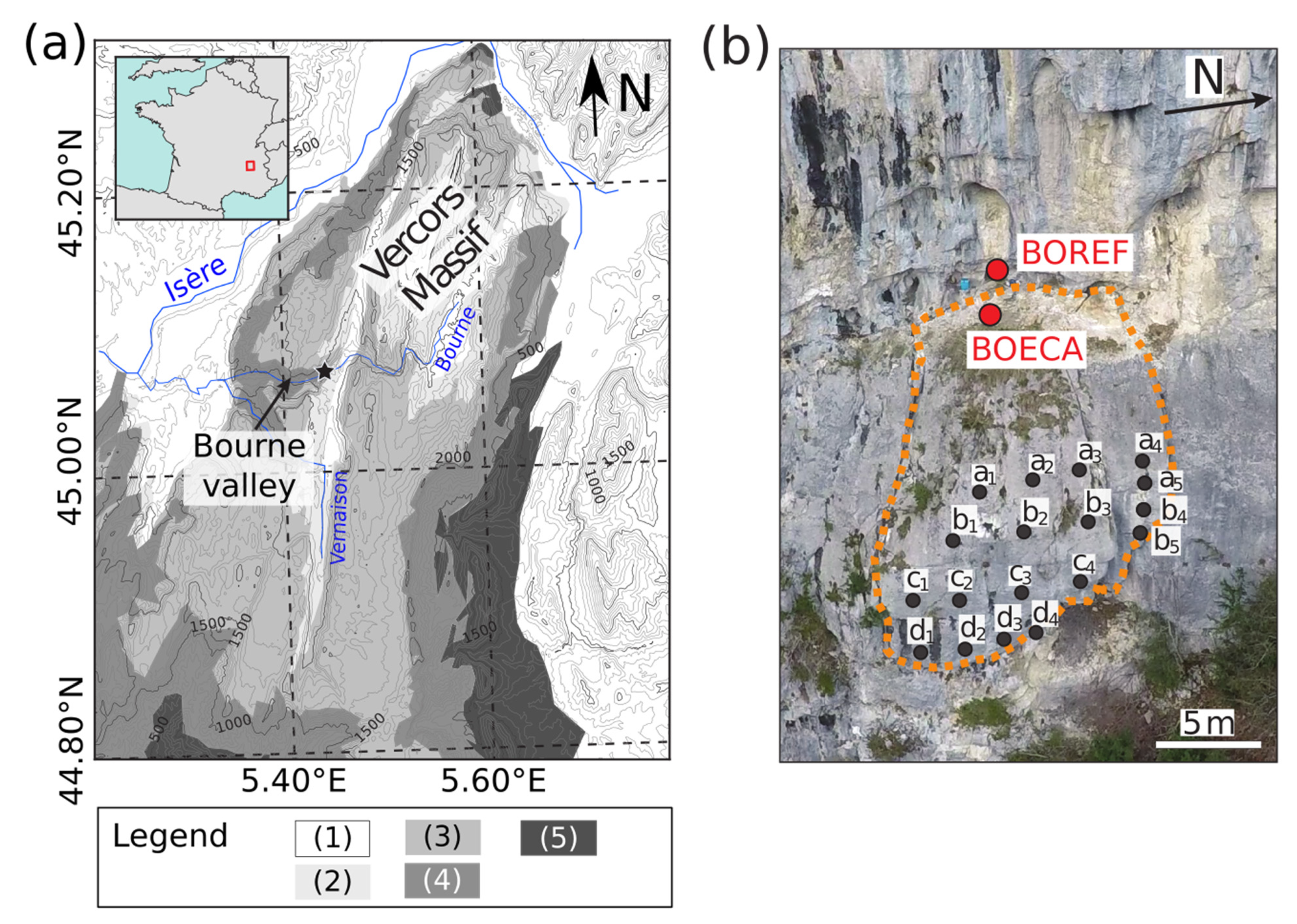
2. Site Description
3. Data Acquisition and Processing
4. Parameter Robustness and Ability to Derive Unstable Column’s Dynamic Parameters
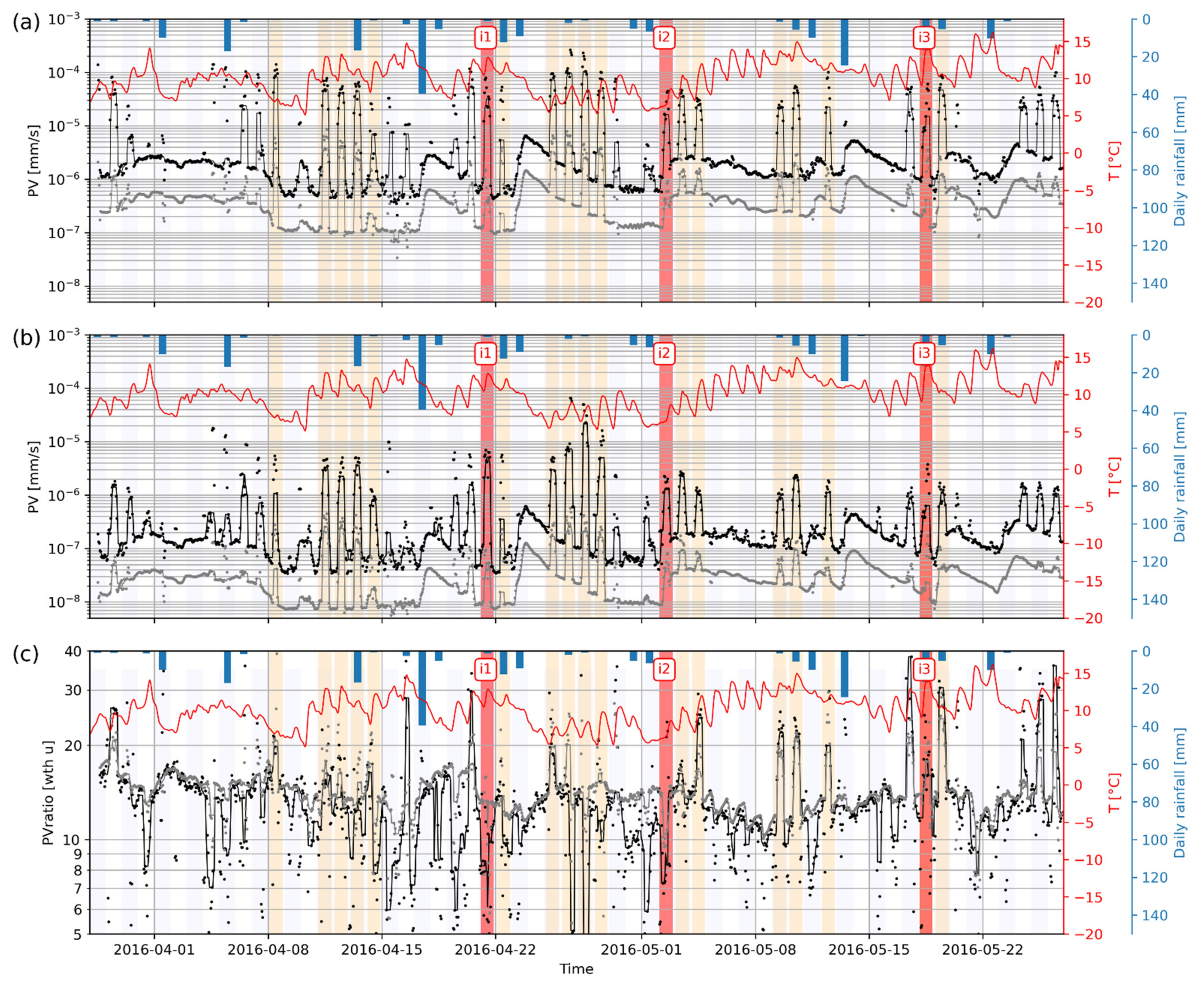
4.1. Particle Velocity Monitoring (PV)
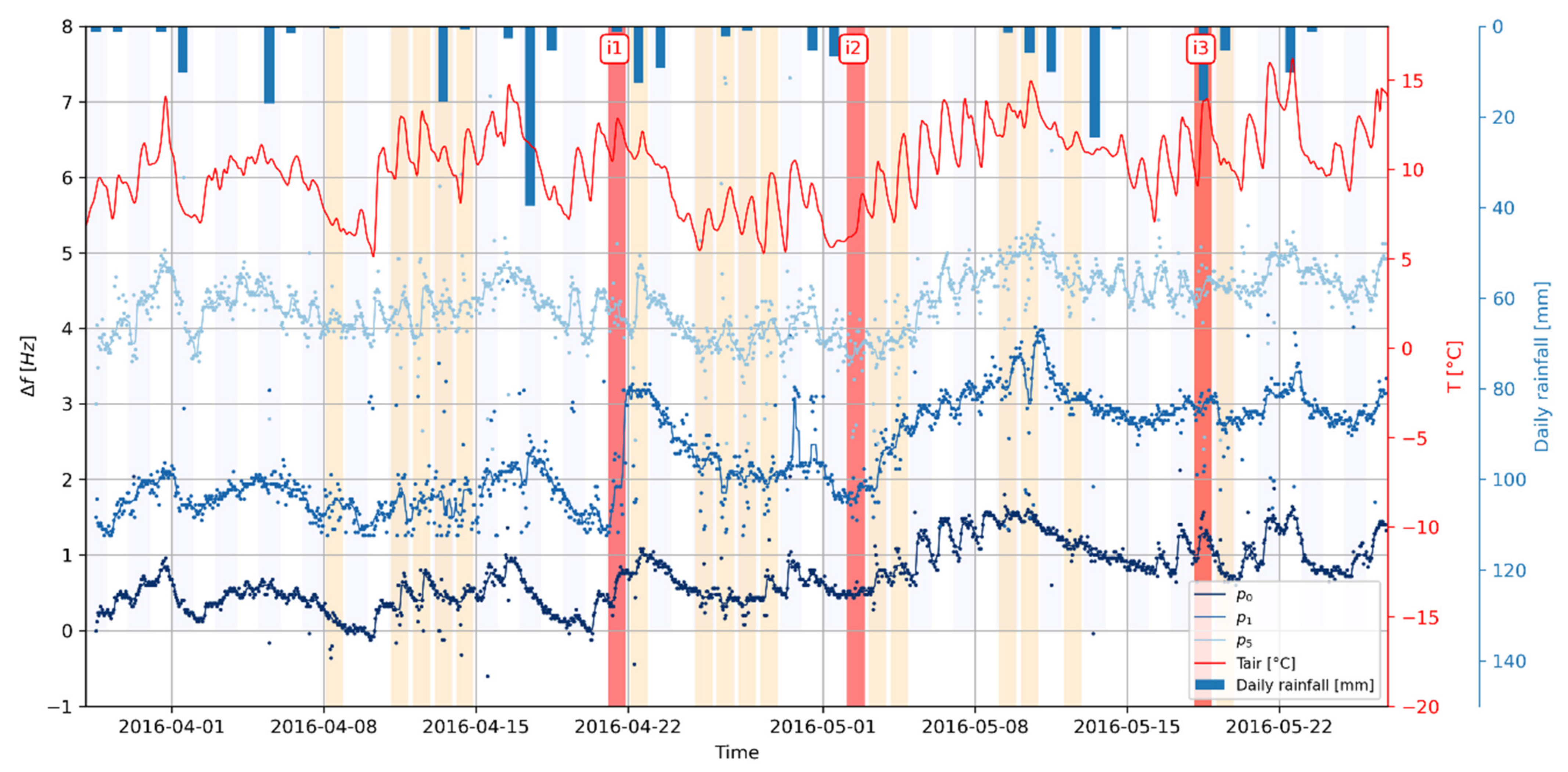
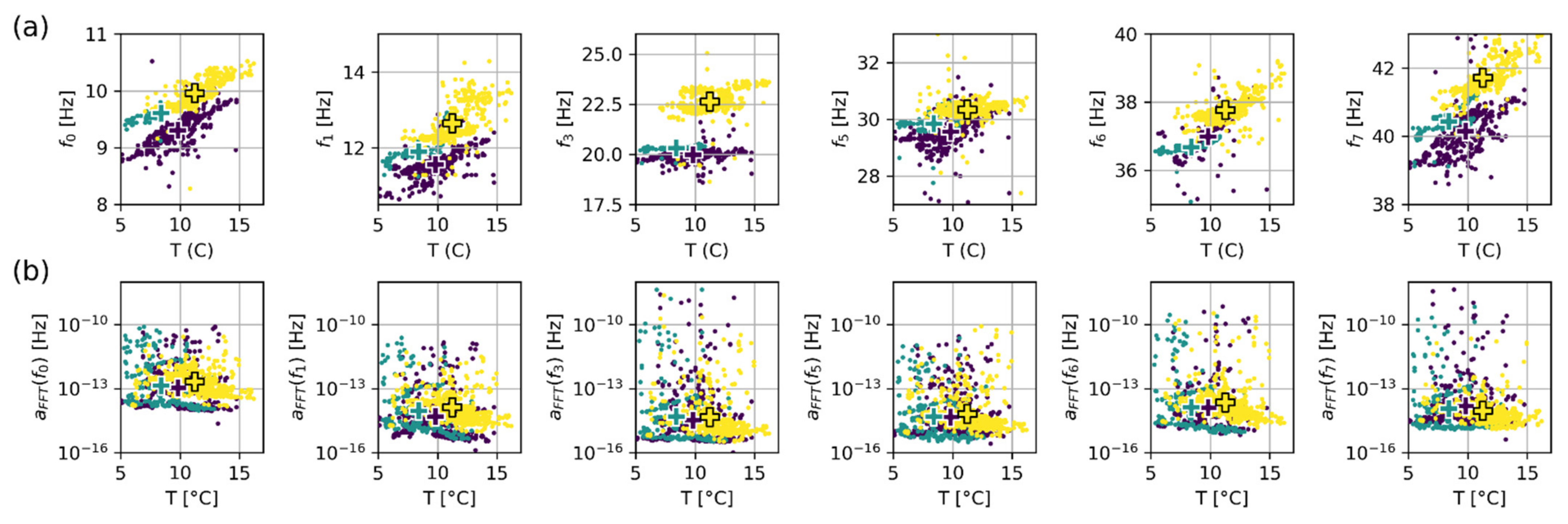
4.2. Spectrum Monitoring
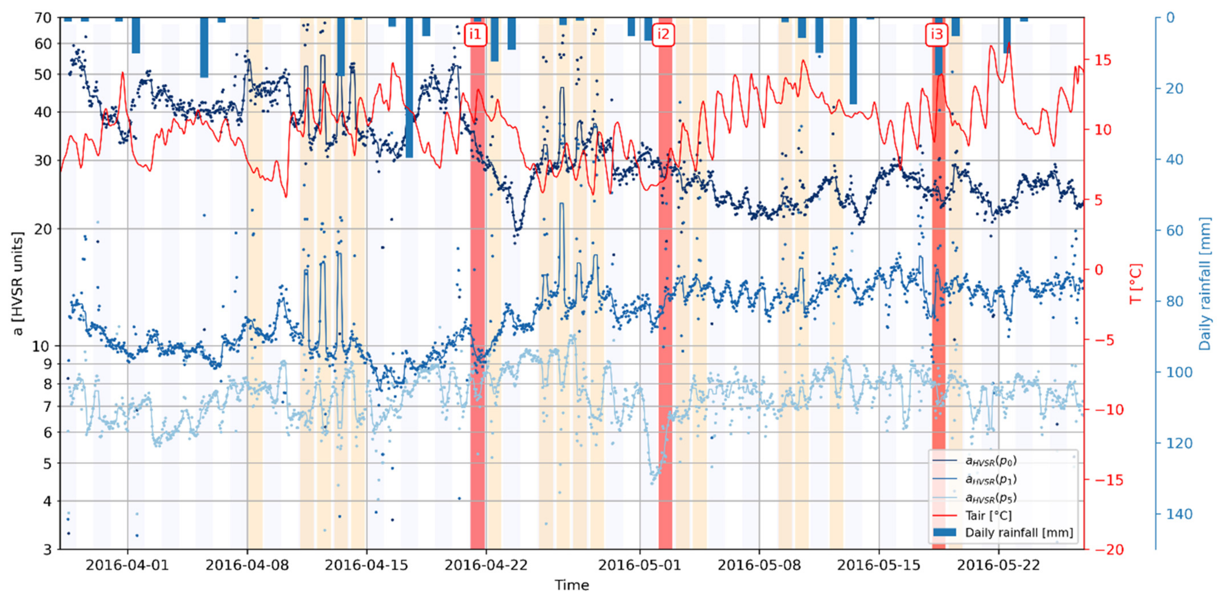
4.3. Horizontal-to-Vertical Spectral Ratio (HVSR) Monitoring
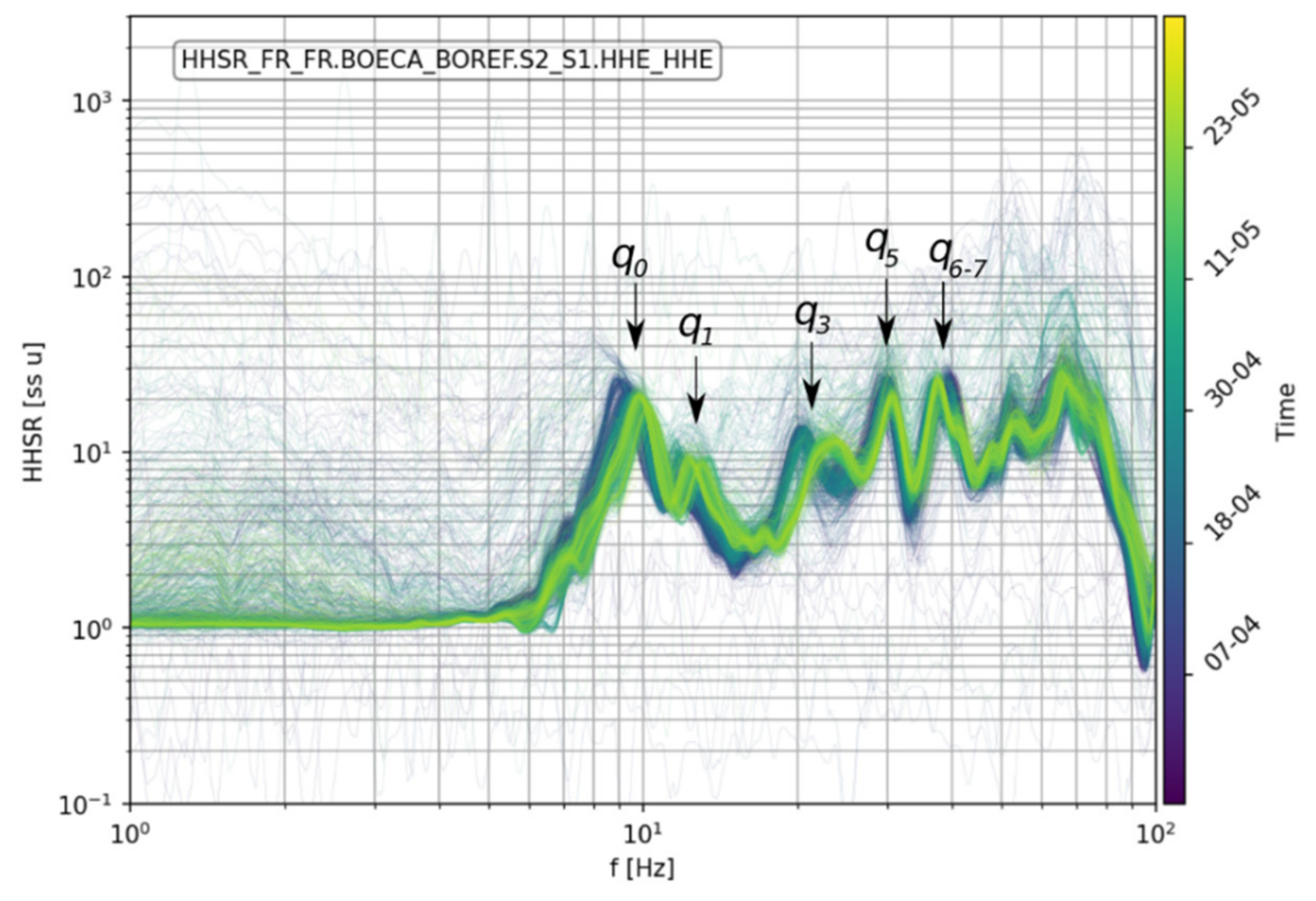
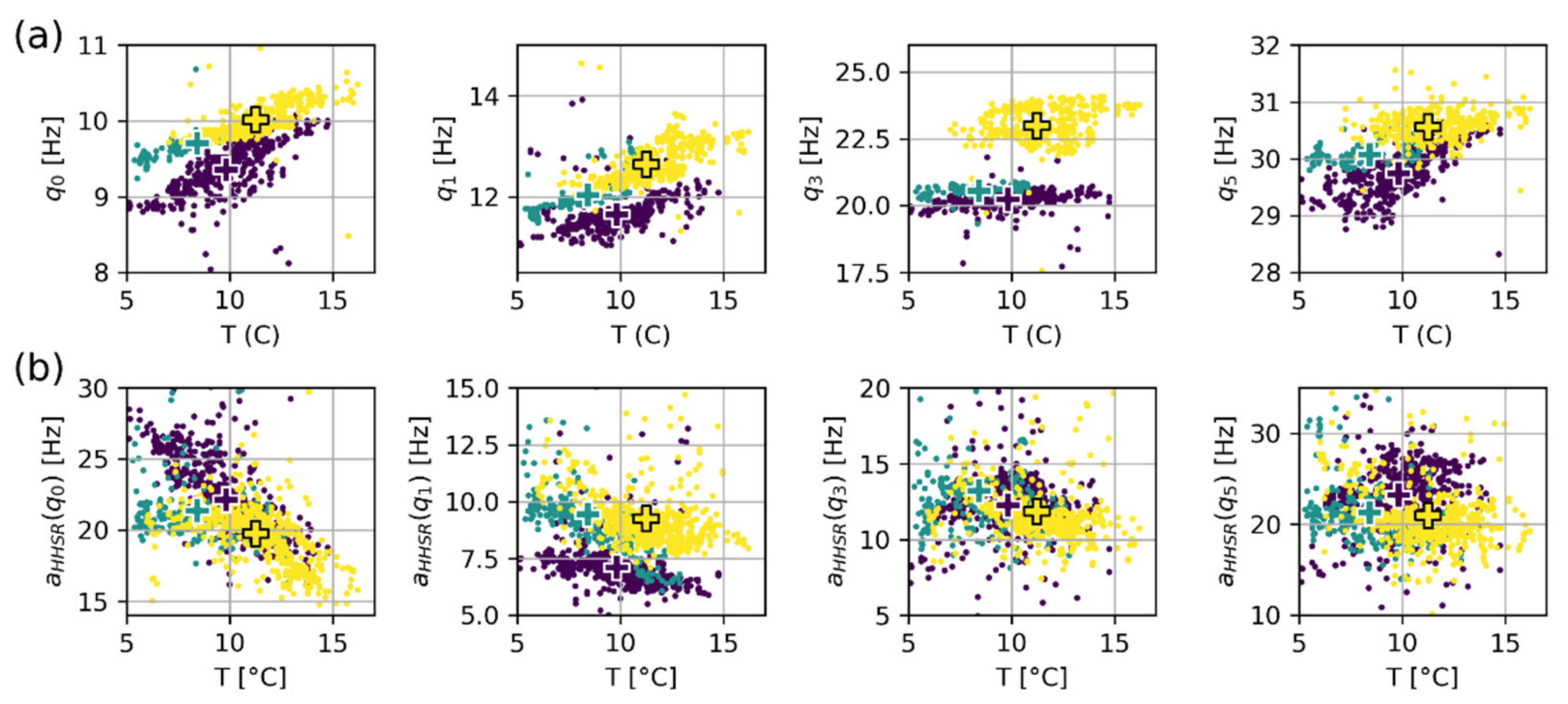
4.4. Horizontal-to-Horizontal Spectral Ratio (HHSR) Monitoring
5. Sensitivity of Seismic Spectra Parameters to Bolting
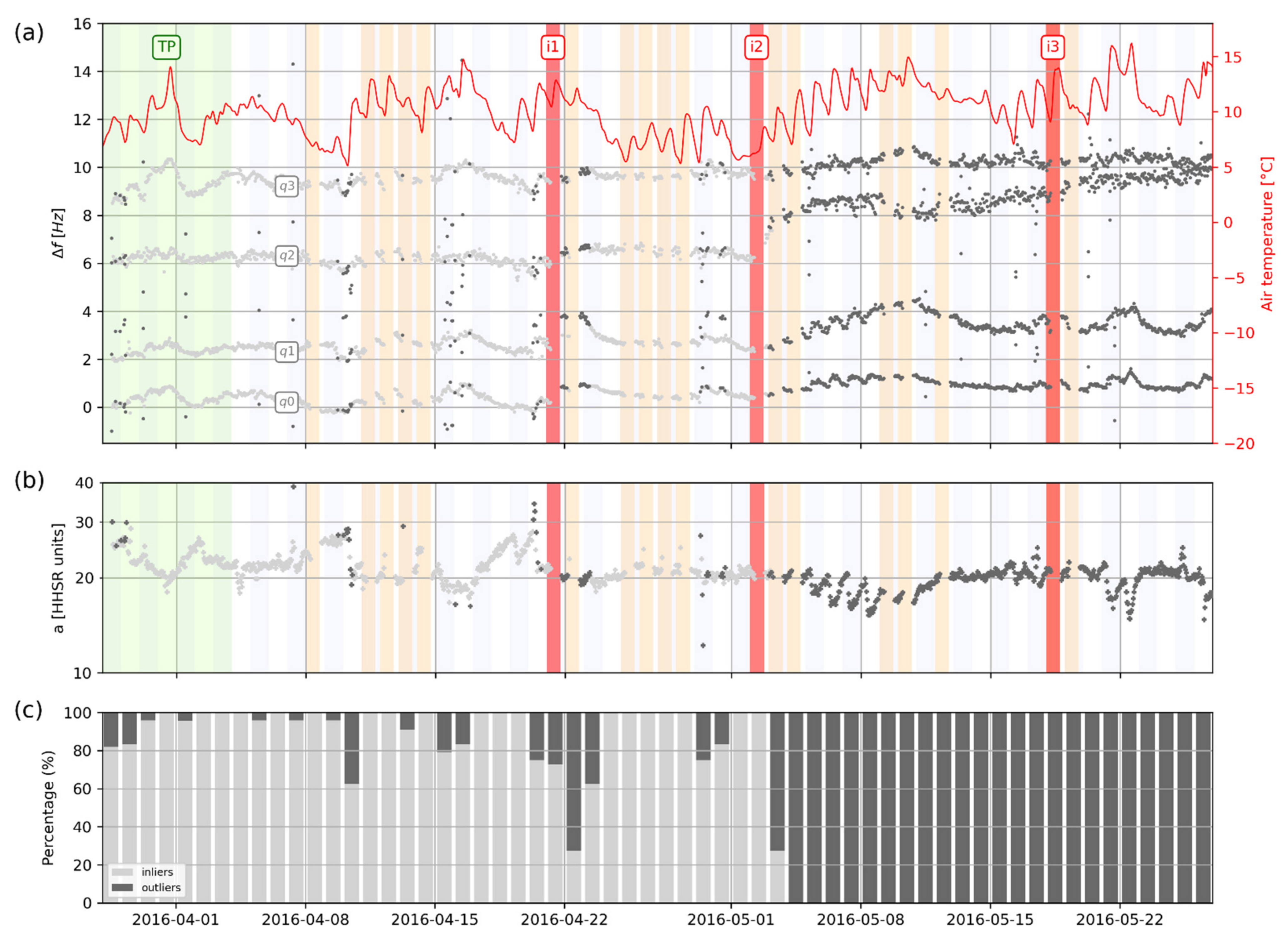
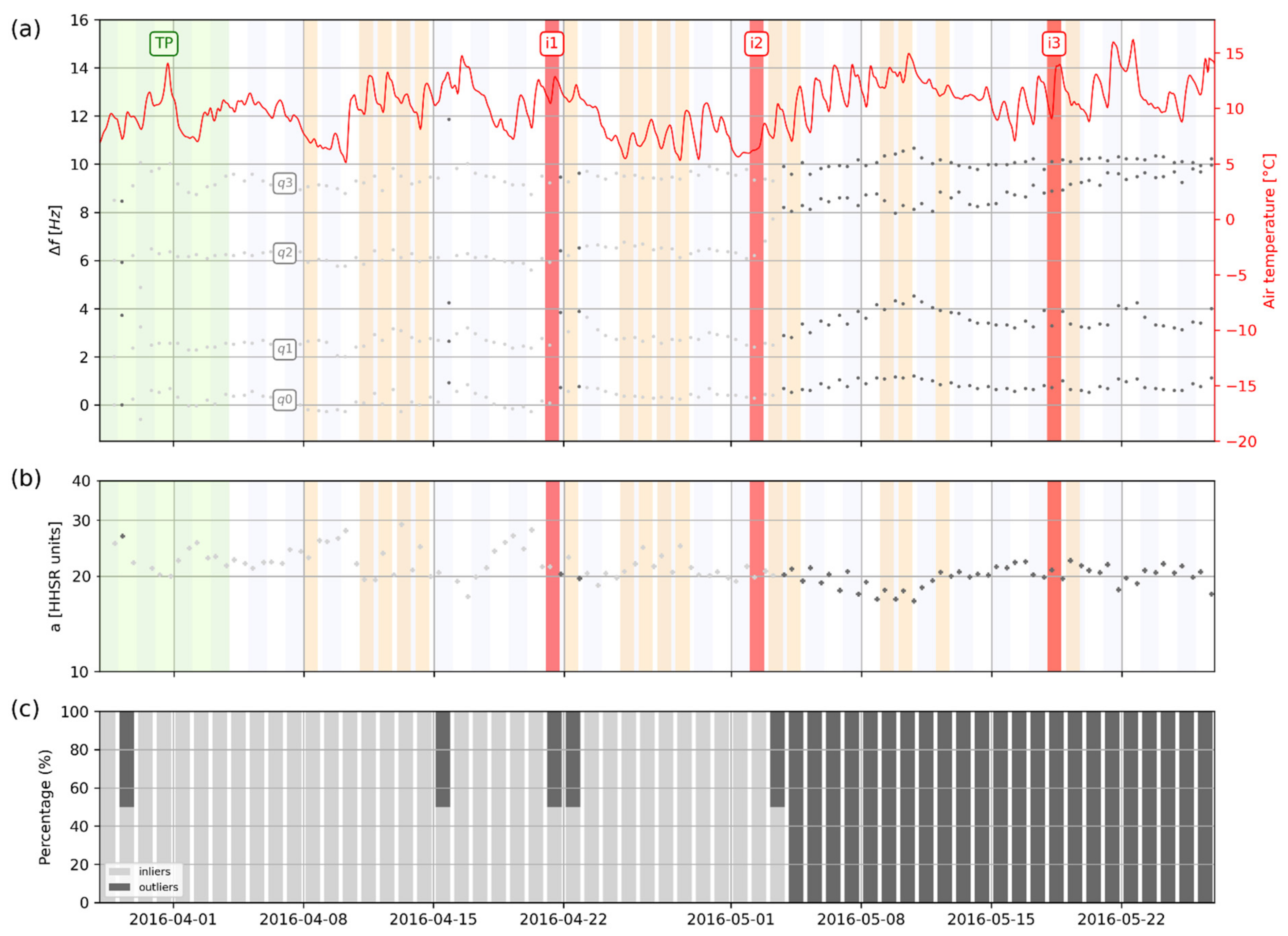
6. Novelty Detection Algorithms
7. Discussion
- -
- The first strategy consists of monitoring as many natural frequencies as possible, e.g., derived from HHSR, which facilitates the peak peaking process due to the normalization of spectral ratio. This assumes that most frequencies will experience significant changes during the monitoring, which is not straightforwardly supported by our results;
- -
- The other strategy consists of monitoring the sole fundamental mode since it represents the global behavior of the prone-to-fall mass. This can be achieved with HVSR or HHSR indistinctively, which show a similar change in fundamental natural frequency.
8. Conclusions
- -
- Spectral estimators such as FFT, HVSR, and HHSR can be used to point out unstable compartment natural frequencies, although the use of HVSR should be restricted to fundamental mode only;
- -
- HHSR appears as a good trade-off between spectral stability and accuracy. HHSR amplitude yet revealed sensitivity to the location of the reference sensor. This sensor should be set close enough to the site to depict the incoming wavefield but far enough from the rock compartment to avoid recording its natural frequencies;
- -
- Column-shape rock compartments with clear rear fracture can be monitored with such lightweight instrumentations that are set up with a reduced number of sensors/channels.
- -
- The automatic Elliptic Envelope routine successfully removed adverse thermomechanical fluctuations affecting the time series. Such fluctuations substantially complicated the operational use of VB–SHM on natural structures until now.
- -
- The novelty detection algorithm performed well on reduced datasets with only a few measurements per day. This suggesting that a triggered-recording scheme (e.g., a few tens of minutes of ambient vibrations recorded each day) could be used for massive power savings;
- -
- Ad hoc, robust, low-cost, and low-power hardware instrumentation with telecommunication ability is now required to facilitate such surveys in remote mountainous areas;
- -
- These promising results for rock bolting detection should also be tested against progressive damage before rockfall.
Author Contributions
Funding
Data Availability Statement
Acknowledgments
Conflicts of Interest
Appendix A


| Parameter | Before i1 | After i1 | After i2 | |
|---|---|---|---|---|
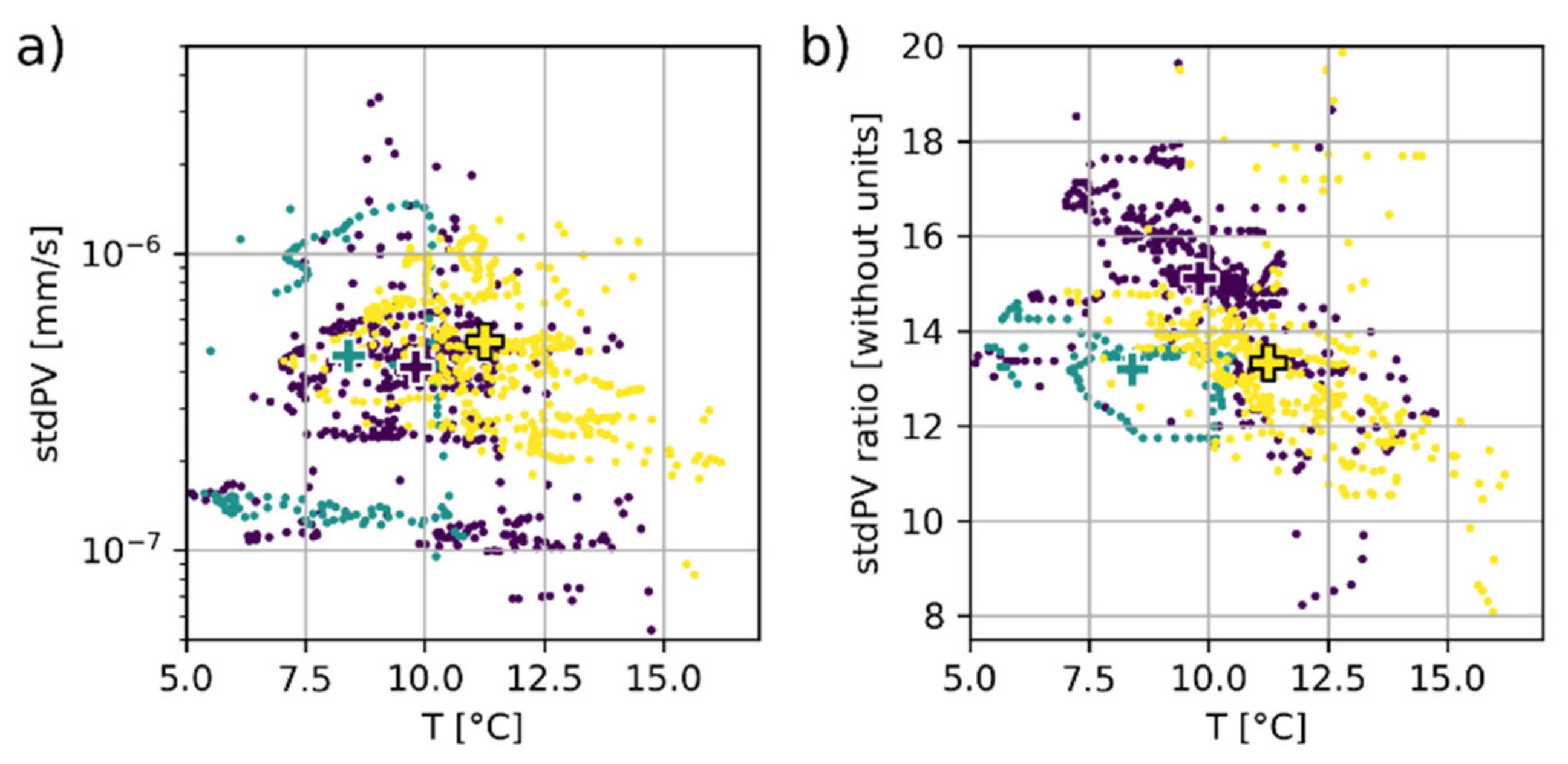
| stdPV on BOECA | Std centroid along freq axis [Hz] | 4.1 × 10⁻⁷ | 4.5 × 10⁻⁷ | 5.1 × 10⁻⁷ |
| Cumulated rise [%] | - | +9.8% | +24.4% | |
| stdPV Ratio between BOECA and BOREF | Std RATIO centroid along freq axis [Hz] | 15.1 | 13.2 | 13.3 |
| Cumulated change [%] | - | −12.6 | −11.9 |
| Parameter | f0 | f1 | f3 | f5 | f6 | f7 | |||||||||||||
|---|---|---|---|---|---|---|---|---|---|---|---|---|---|---|---|---|---|---|---|
| Before i1 | After i1 | After i1 | Before i1 | After i1 | After i2 | Before i1 | After i1 | After i2 | Before i1 | After i1 | After i2 | Before i1 | After i1 | After i2 | Before i1 | After i1 | After i2 | ||
| Peak Frequency | Centroid position along f [Hz] | 9.3 | 9.6 | 10.0 | 11.6 | 11.9 | 12.7 | 20.0 | 20.3 | 22.6 | 29.6 | 29.8 | 30.3 | 37.0 | 36.7 | 37.8 | 40.2 | 40.4 | 41.7 |
| Cumulated rise [%] | - | +3.2 | +7.5 | - | +2.6 | +9.5 | - | +1.5 | +13.0 | - | +0.7 | +2.4 | - | −0.8 | +2.2 | - | +0.5 | +3.7 | |
| Peak Amplitude | Centroid position along a [FFT units] | 1.1 × 10⁻¹³ | 1.4 × 10⁻¹³ | 2.1 × 10⁻¹³ | 4.8 × 10⁻¹⁵ | 9.2 × 10⁻¹⁵ | 1.3 × 10⁻¹⁴ | 3.4 × 10⁻¹⁵ | 4.8 × 10⁻¹⁵ | 4.7 × 10⁻¹⁵ | 4.5 × 10⁻¹⁵ | 4.8 × 10⁻¹⁵ | 6.5 × 10⁻¹⁵ | 1.3 × 10⁻¹⁴ | 1.3 × 10⁻¹⁴ | 2.2 × 10⁻¹⁴ | 1.5 × 10⁻¹⁴ | 1.1 × 10⁻¹⁴ | 9.1 × 10⁻¹⁵ |
| Cumulated rise [%] | - | +27.3 | +91 | - | +92 | +171 | - | +41.2 | +38.2 | - | +6.7 | +44 | - | 0 | +69 | - | −26.7 | −39 | |
| Parameter | p0 | p1 | p5 | |||||||
|---|---|---|---|---|---|---|---|---|---|---|
| Before i1 | After i1 | After i2 | Before i1 | After i1 | After i2 | Before i1 | After i1 | After i2 | ||
| Peak Frequency | Centroid position along f[Hz] | 9.3 | 9.6 | 10.0 | 11.6 | 12.2 | 12.7 | 29.9 | 29.7 | 30.3 |
| Cumulated rise [%] | - | +3.2 | +7.5 | - | +5.2 | +9.5 | - | −0.7 | +1.3 | |
| Peak Amplitude | Centroid position along a [without units] | 40.4 | 30.5 | 24.7 | 10.3 | 13.0 | 14.0 | 7.1 | 7.8 | 7.5 |
| Cumulated rise [%] | - | −25 | −39 | - | +26.2 | +36 | - | +9.9 | +5.6 | |
| Parameter | q0 | q1 | q3 | q5 | |||||||||
|---|---|---|---|---|---|---|---|---|---|---|---|---|---|
| Before i1 | After i1 | After i2 | Before i1 | After i1 | After i2 | Before i1 | After i1 | After i2 | Before i1 | After i1 | After i2 | ||
| Peak Frequency | Centroid position along f[Hz] | 9.4 | 9.7 | 10.0 | 11.6 | 12.0 | 12.6 | 20.2 | 20.6 | 23.0 | 29.7 | 30.1 | 30.6 |
| Cumulated rise [%] | - | +3.2 | +6.4 | - | +3.5 | +8.6 | - | +2.0 | +13.9 | - | +1.4 | +3.0 | |
| Peak Amplitude | Centroid position along a [without units] | 22.1 | 21.3 | 19.7 | 7.1 | 9.4 | 9.2 | 12.3 | 13.2 | 11.8 | 23.2 | 21.3 | 21.0 |
| Cumulated rise [%] | - | −3.6 | −10.9 | - | +32.4 | +29.6 | - | +7.3 | −4.1 | - | −8.2 | −9.5 | |
Appendix B. Ambient Vibration Particle Velocity (PV)


References
- Chang, F.-K. Structural Health Monitoring 2000; CRC Press: Boca Raton, FL, USA, 1999; ISBN 978-1-56676-881-8. [Google Scholar]
- Farrar, C.R.; Worden, K. An Introduction to Structural Health Monitoring. In New Trends in Vibration Based Structural Health Monitoring; Deraemaeker, A., Worden, K., Eds.; CISM Courses and Lectures; Springer: Vienna, Austria, 2010; pp. 1–17. ISBN 978-3-7091-0399-9. [Google Scholar]
- Farrar, C.R.; Worden, K. Structural Health Monitoring: A Machine Learning Perspective; John Wiley & Sons: Hoboken, NJ, USA, 2012; ISBN 978-1-118-44321-7. [Google Scholar]
- Humar, J.L.; Amin, M.S. Structural Health Monitoring. In Structural Engineering, Mechanics and Computation; Zingoni, A., Ed.; Elsevier Science: Oxford, UK, 2001; pp. 1185–1193. ISBN 978-0-08-043948-8. [Google Scholar]
- Balageas, D.; Fritzen, C.-P.; Güemes, A. Structural Health Monitoring; John Wiley & Sons: Hoboken, NJ, USA, 2010; ISBN 978-0-470-39440-3. [Google Scholar]
- Ostachowicz, W.; Güemes, A. New Trends in Structural Health Monitoring; Springer Science & Business Media: Berlin/Heidelberg, Germany, 2013; ISBN 978-3-7091-1390-5. [Google Scholar]
- Fu, Z.-F.; He, J. Modal Analysis; Elsevier: Amsterdam, The Netherlands, 2001. [Google Scholar]
- Brincker, R.; Ventura, C. Introduction to Operational Modal Analysis; John Wiley & Sons: Hoboken, NJ, USA, 2015; ISBN 978-1-119-96315-8. [Google Scholar]
- Avitabile, P. Experimental Modal Analysis. J. Sound Vib. 2001, 35, 20–31. [Google Scholar]
- Cunha, Á.; Caetano, E.; Magalhães, F.; Moutinho, C. From Input-Output to Output-Only Modal Identification of Civil Engineering Structures. In Proceedings of the 1st International Operational Modal Analysis Conference (IOMAC), Copenhagen, Denmark, 26–27 April 2005; p. 22. [Google Scholar]
- He, Q.; Ding, X. Time-Frequency Manifold for Machinery Fault Diagnosis. In Structural Health Monitoring: An Advanced Signal Processing Perspective; Yan, R., Chen, X., Mukhopadhyay, S.C., Eds.; Smart Sensors, Measurement and Instrumentation; Springer International Publishing: Cham, Switzerland, 2017; pp. 131–154. ISBN 978-3-319-56126-4. [Google Scholar]
- Tang, G.; Wang, H.; Ke, Y.; Luo, G. Compressive Sensing: A New Insight to Condition Monitoring of Rotary Machinery. In Structural Health Monitoring: An Advanced Signal Processing Perspective; Yan, R., Chen, X., Mukhopadhyay, S.C., Eds.; Smart Sensors, Measurement and Instrumentation; Springer International Publishing: Cham, Switzerland, 2017; pp. 203–225. ISBN 978-3-319-56126-4. [Google Scholar]
- Chen, X.; Wang, S. Matching Demodulation Transform and Its Application in Machine Fault Diagnosis. In Structural Health Monitoring: An Advanced Signal Processing Perspective; Yan, R., Chen, X., Mukhopadhyay, S.C., Eds.; Smart Sensors, Measurement and Instrumentation; Springer International Publishing: Cham, Switzerland, 2017; pp. 155–202. ISBN 978-3-319-56126-4. [Google Scholar]
- Lei, Y. Fault Diagnosis of Rotating Machinery Based on Empirical Mode Decomposition. In Structural Health Monitoring: An Advanced Signal Processing Perspective; Yan, R., Chen, X., Mukhopadhyay, S.C., Eds.; Smart Sensors, Measurement and Instrumentation; Springer International Publishing: Cham, Switzerland, 2017; pp. 259–292. ISBN 978-3-319-56126-4. [Google Scholar]
- Sohn, H.; Farrar, C.R.; Hemez, F.M.; Czarnecki, J.J. A Review of Structural Health Review of Structural Health Monitoring Literature 1996–2001; Los Alamos National Lab. (LANL): Los Alamos, NM, USA, 2002. [Google Scholar]
- Chang, F.-K.; Markmiller, J.F.C.; Yang, J.; Kim, Y. Structural Health Monitoring. In System Health Management; John Wiley & Sons, Ltd.: Hoboken, NJ, USA, 2011; pp. 419–428. ISBN 978-1-119-99405-3. [Google Scholar]
- Lorenzoni, F.; Casarin, F.; Caldon, M.; Islami, K.; Modena, C. Uncertainty Quantification in Structural Health Monitoring: Applications on Cultural Heritage Buildings. Mech. Syst. Signal Process. 2016, 66–67, 268–281. [Google Scholar] [CrossRef]
- De Stefano, A.; Matta, E.; Clemente, P. Structural Health Monitoring of Historical Heritage in Italy: Some Relevant Experiences. J. Civ. Struct. Health Monit. 2016, 6, 83–106. [Google Scholar] [CrossRef]
- Lorenzoni, F.; Caldon, M.; da Porto, F.; Modena, C.; Aoki, T. Post-Earthquake Controls and Damage Detection through Structural Health Monitoring: Applications in l’Aquila. J. Civ. Struct. Health Monit. 2018, 8, 217–236. [Google Scholar] [CrossRef]
- Brownjohn, J.M.W. Structural Health Monitoring of Civil Infrastructure. Philos. Trans. R. Soc. A Math. Phys. Eng. Sci. 2007, 365, 589–622. [Google Scholar] [CrossRef] [PubMed]
- Clinton, J.F.; Bradford, S.C.; Heaton, T.H.; Favela, J. The Observed Wander of the Natural Frequencies in a Structure. Bull. Seismol. Soc. Am. 2006, 96, 237–257. [Google Scholar] [CrossRef]
- Bradford, S.C.; Clinton, J.F.; Favela, J.; Heaton, T.H. Results of Millikan Library Forced Vibration Testing; Technical Report; California Institute of Technology: Pasadena, CA, USA, 2004. [Google Scholar]
- Michel, C.; Guéguen, P.; El Arem, S.; Mazars, J.; Kotronis, P. Full-Scale Dynamic Response of an RC Building under Weak Seismic Motions Using Earthquake Recordings, Ambient Vibrations and Modelling. Earthq. Eng. Struct. Dyn. 2010, 39, 419–441. [Google Scholar] [CrossRef]
- Michel, C.; Guéguen, P.; Bard, P.-Y. Dynamic Parameters of Structures Extracted from Ambient Vibration Measurements: An Aid for the Seismic Vulnerability Assessment of Existing Buildings in Moderate Seismic Hazard Regions. Soil Dyn. Earthq. Eng. 2008, 28, 593–604. [Google Scholar] [CrossRef]
- Mucciarelli, M.; Masi, A.; Gallipoli, M.R.; Harabaglia, P.; Vona, M.; Ponzo, F.; Dolce, M. Analysis of RC Building Dynamic Response and Soil-Building Resonance Based on Data Recorded during a Damaging Earthquake (Molise, Italy, 2002). Bull. Seismol. Soc. Am. 2004, 94, 1943–1953. [Google Scholar] [CrossRef]
- Peeters, B.; Maeck, J.; De Roeck, G. Vibration-Based Damage Detection in Civil Engineering: Excitation Sources and Temperature Effects. Smart Mater. Struct. 2001, 10, 518. [Google Scholar] [CrossRef]
- Farrar, C.R.; Cone, K.M. Vibration Testing of the I-40 Bridge before and after the Introduction of Damage; Los Alamos National Lab.: Los Alamos, NM, USA, 1994.
- Glisic, B.; Inaudi, D. Fibre Optic Methods for Structural Health Monitoring; John Wiley & Sons: Hoboken, NJ, USA, 2008; ISBN 978-0-470-51780-2. [Google Scholar]
- Rivera, E.; Mufti, A.A.; Thomson, D.J. Civionics for Structural Health Monitoring. Can. J. Civ. Eng. 2011, 34, 430–437. [Google Scholar] [CrossRef]
- Kim, S.; Pakzad, S.; Culler, D.; Demmel, J.; Fenves, G.; Glaser, S.; Turon, M. Wireless Sensor Networks for Structural Health Monitoring. In Proceedings of the 4th International Conference on Embedded Networked Sensor Systems (SenSys ’06), Boulder, CO, USA, NY, USA, 31 October–3 November 2006; Association for Computing Machinery: New York, NY, USA; pp. 427–428. [Google Scholar] [CrossRef]
- Lynch, J.; Loh, K. A Summary Review of Wireless Sensors and Sensor Networks for Structural Health Monitoring. Shock Vib. Dig. 2006, 38, 91–128. [Google Scholar] [CrossRef]
- Nagayama, T.; Spencer, B.F., Jr. Structural Health Monitoring Using Smart Sensors; Newmark Structural Engineering Laboratory, University of Illinois at Urbana-Champaign: Urbana, IL, USA, 2007. [Google Scholar]
- Worden, K.; Manson, G. The Application of Machine Learning to Structural Health Monitoring. Philos. Trans. R. Soc. A Math. Phys. Eng. Sci. 2007, 365, 515–537. [Google Scholar] [CrossRef] [PubMed]
- Abdeljaber, O.; Avci, O.; Kiranyaz, M.S.; Boashash, B.; Sodano, H.; Inman, D.J. 1-D CNNs for Structural Damage Detection: Verification on a Structural Health Monitoring Benchmark Data. Neurocomputing 2018, 275, 1308–1317. [Google Scholar] [CrossRef]
- Roux, P.; Guéguen, P.; Baillet, L.; Hamze, A. Structural-Change Localization and Monitoring through a Perturbation-Based Inverse Problem. J. Acoust. Soc. Am. 2014, 136, 2586–2597. [Google Scholar] [CrossRef] [PubMed]
- Sohn, H.; Czarnecki, J.A.; Farrar, C.R. Structural Health Monitoring Using Statistical Process Control. J. Struct. Eng. 2000, 126, 1356–1363. [Google Scholar] [CrossRef]
- Roy, K.; Bhattacharya, B.; Ray Chaudhuri, S. ARX Model-Based Damage Sensitive Features for Structural Damage Localization Using Output-Only Measurements. J. Sound Vib. 2015, 349, 99–122. [Google Scholar] [CrossRef]
- Hu, W.-H.; Cunha, Á.; Caetano, E.; Rohrmann, R.G.; Said, S.; Teng, J. Comparison of Different Statistical Approaches for Removing Environmental/Operational Effects for Massive Data Continuously Collected from Footbridges. Struct. Control Health Monit. 2017, 24, e1955. [Google Scholar] [CrossRef]
- Çelebi, M. Seismic Responses of Two Adjacent Buildings. I: Data and Analyses. J. Struct. Eng. 1993, 119, 2461–2476. [Google Scholar] [CrossRef]
- Ivanović, S.S.; Trifunac, M.D.; Novikova, E.I.; Gladkov, A.A.; Todorovska, M.I. Ambient Vibration Tests of a Seven-Story Reinforced Concrete Building in Van Nuys, California, Damaged by the 1994 Northridge Earthquake. Soil Dyn. Earthq. Eng. 2000, 19, 391–411. [Google Scholar] [CrossRef]
- Dunand, F.; Gueguen, P.; Bard, P.-Y.; Rodgers, J. Comparison of the Dynamic Parameters Extracted from Weak, Moderate and Strong Building Motion. In Proceedings of the First European Conference on Earthquake Engineering and Seismology, Geneva, Switzerland, 3–8 September 2006. [Google Scholar]
- Verma, R.K.; Pattanaik, K.K.; Dissanayake, P.B.R.; Dammika, A.J.; Buddika, H.A.D.S.; Kaloop, M.R. Damage Detection in Bridge Structures: An Edge Computing Approach. arXiv 2020, arXiv:2008.06724. [Google Scholar]
- Avci, O.; Abdeljaber, O.; Kiranyaz, S.; Hussein, M.; Inman, D.J. Wireless and Real-Time Structural Damage Detection: A Novel Decentralized Method for Wireless Sensor Networks. J. Sound Vib. 2018, 424, 158–172. [Google Scholar] [CrossRef]
- Starr, A.M.; Moore, J.R.; Thorne, M.S. Ambient Resonance of Mesa Arch, Canyonlands National Park, Utah. Geophys. Res. Lett. 2015, 42, 6696–6702. [Google Scholar] [CrossRef]
- Moore, J.R.; Thorne, M.S.; Koper, K.D.; Wood, J.R.; Goddard, K.; Burlacu, R.; Doyle, S.; Stanfield, E.; White, B. Anthropogenic Sources Stimulate Resonance of a Natural Rock Bridge. Geophys. Res. Lett. 2016, 43, 9669–9676. [Google Scholar] [CrossRef]
- Moore, J.R.; Geimer, P.R.; Finnegan, R.; Thorne, M.S. Use of Seismic Resonance Measurements to Determine the Elastic Modulus of Freestanding Rock Masses. Rock Mech. Rock Eng. 2018, 51, 3937–3944. [Google Scholar] [CrossRef]
- Moore, J.R.; Geimer, P.R.; Finnegan, R.; Michel, C. Dynamic Analysis of a Large Freestanding Rock Tower (Castleton Tower, Utah) Short Note. Bull. Seismol. Soc. Am. 2019, 109, 2125–2131. [Google Scholar] [CrossRef]
- Bottelin, P.; Jongmans, D.; Baillet, L.; Lebourg, T.; Hantz, D.; Lévy, C.; Le Roux, O.; Cadet, H.; Lorier, L.; Rouiller, J.-D. Spectral Analysis of Prone-to-Fall Rock Compartments Using Ambient Vibrations. J. Environ. Eng. Geophys. 2013, 18, 205–217. [Google Scholar] [CrossRef]
- Bottelin, P.; Lévy, C.; Baillet, L.; Jongmans, D.; Gueguen, P. Modal and Thermal Analysis of Les Arches Unstable Rock Column (Vercors Massif, French Alps). Geophys. J. Int. 2013, 194, 849–858. [Google Scholar] [CrossRef]
- Valentin, J.; Capron, A.; Jongmans, D.; Baillet, L.; Bottelin, P.; Donze, F.; Larose, E.; Mangeney, A. The Dynamic Response of Prone-to-Fall Columns to Ambient Vibrations: Comparison between Measurements and Numerical Modelling. Geophys. J. Int. 2017, 208, 1058–1076. [Google Scholar] [CrossRef]
- Moore, J.R.; Gischig, V.; Burjánek, J.; Loew, S.; Fäh, D. Site Effects in Unstable Rock Slopes: Dynamic Behavior of the Randa Instability (Switzerland). Bull. Seismol. Soc. Am. 2011, 101, 3110–3116. [Google Scholar] [CrossRef]
- Burjánek, J.; Gassner-Stamm, G.; Poggi, V.; Moore, J.R.; Fäh, D. Ambient Vibration Analysis of an Unstable Mountain Slope. Geophys. J. Int. 2010, 180, 820–828. [Google Scholar] [CrossRef]
- Burjánek, J.; Moore, J.R.; Yugsi Molina, F.X.; Fäh, D. Instrumental Evidence of Normal Mode Rock Slope Vibration. Geophys. J. Int. 2012, 188, 559–569. [Google Scholar] [CrossRef]
- Kleinbrod, U.; Burjánek, J.; Hugentobler, M.; Amann, F.; Fäh, D. A Comparative Study on Seismic Response of Two Unstable Rock Slopes within Same Tectonic Setting but Different Activity Level. Geophys. J. Int. 2017, 211, 1428–1448. [Google Scholar] [CrossRef]
- Kleinbrod, U.; Burjánek, J.; Fäh, D. Ambient Vibration Classification of Unstable Rock Slopes: A Systematic Approach. Eng. Geol. 2019, 249, 198–217. [Google Scholar] [CrossRef]
- Lévy, C.; Jongmans, D.; Baillet, L. Analysis of Seismic Signals Recorded on a Prone-to-Fall Rock Column (Vercors Massif, French Alps). Geophys. J. Int. 2011, 186, 296–310. [Google Scholar] [CrossRef]
- Burjánek, J.; Gischig, V.; Moore, J.R.; Fäh, D. Ambient Vibration Characterization and Monitoring of a Rock Slope Close to Collapse. Geophys. J. Int. 2018, 212, 297–310. [Google Scholar] [CrossRef]
- Burjánek, J.; Edwards, B.; Fäh, D. Empirical Evidence of Local Seismic Effects at Sites with Pronounced Topography: A Systematic Approach. Geophys. J. Int. 2014, 197, 608–619. [Google Scholar] [CrossRef]
- Häusler, M.; Michel, C.; Burjánek, J.; Fäh, D. Fracture Network Imaging on Rock Slope Instabilities Using Resonance Mode Analysis. Geophys. Res. Lett. 2019, 46, 6497–6506. [Google Scholar] [CrossRef]
- Hollender, F.; Roumelioti, Z.; Maufroy, E.; Traversa, P.; Mariscal, A. Can We Trust High-Frequency Content in Strong-Motion Database Signals? Impact of Housing, Coupling, and Installation Depth of Seismic Sensors. Seismol. Res. Lett. 2020, 91, 2192–2205. [Google Scholar] [CrossRef]
- Gischig, V.S.; Eberhardt, E.; Moore, J.R.; Hungr, O. On the Seismic Response of Deep-Seated Rock Slope Instabilities—Insights from Numerical Modeling. Eng. Geol. 2015, 193, 1–18. [Google Scholar] [CrossRef]
- Weber, S.; Fäh, D.; Beutel, J.; Faillettaz, J.; Gruber, S.; Vieli, A. Ambient Seismic Vibrations in Steep Bedrock Permafrost Used to Infer Variations of Ice-Fill in Fractures. Earth Planet. Sci. Lett. 2018, 501, 119–127. [Google Scholar] [CrossRef]
- Cooley, J.W.; Tukey, J.W. An Algorithm for the Machine Calculation of Complex Fourier Series. Math. Comp. 1965, 19, 297. [Google Scholar] [CrossRef]
- Lévy, C.; Baillet, L.; Jongmans, D.; Mourot, P.; Hantz, D. Dynamic Response of the Chamousset Rock Column (Western Alps, France). J. Geophys. Res. Earth Surf. 2010, 115, F04043. [Google Scholar] [CrossRef]
- Welch, P. The Use of Fast Fourier Transform for the Estimation of Power Spectra: A Method Based on Time Averaging over Short, Modified Periodograms. IEEE Trans. Audio Electroacoust. 1967, AU-15, 70–73. [Google Scholar] [CrossRef]
- McNamara, D.E.; Buland, R.P. Ambient Noise Levels in the Continental United States. Bull. Seismol. Soc. Am. 2004, 94, 1517–1527. [Google Scholar] [CrossRef]
- Prieto, G.A.; Parker, R.L.; Vernon, F.L., III. A Fortran 90 Library for Multitaper Spectrum Analysis. Comput. Geosci. 2009, 35, 1701–1710. [Google Scholar] [CrossRef]
- Vidale, J.E. Complex Polarization Analysis of Particle Motion. Bull. Seismol. Soc. Am. 1986, 76, 1393–1405. [Google Scholar]
- Torrence, C.; Compo, G.P. A Practical Guide to Wavelet Analysis. Bull. Am. Meteorol. Soc. 1998, 79, 61–78. [Google Scholar] [CrossRef]
- Koper, K.D.; Hawley, V.L. Frequency Dependent Polarization Analysis of Ambient Seismic Noise Recorded at a Broadband Seismometer in the Central United States. Earthq. Sci. 2010, 23, 439–447. [Google Scholar] [CrossRef]
- Koper, K.D.; Burlacu, R. The Fine Structure of Double-Frequency Microseisms Recorded by Seismometers in North America. J. Geophys. Res. Solid Earth 2015, 120, 1677–1691. [Google Scholar] [CrossRef]
- Bard, P.Y.; Acerra, C.; Aguacil, G.; Anastasiadis, A.; Atakan, K.; Azzara, R.M.; Basili, R.; Bertrand, E.; Bettig, B.; Blarel, F.; et al. Guidelines for the Implementation of the H/V Spectral Ratio Technique on Ambient Vibrations-Measurements, Processing and Interpretations. Bull. Earthq. Eng. 2008, 6, 1–2. [Google Scholar] [CrossRef]
- Lermo, J.; Chávez-García, F.J. Site Effect Evaluation Using Spectral Ratios with Only One Station. Bull. Seismol. Soc. Am. 1993, 83, 1574–1594. [Google Scholar]
- Nakamura, Y. Clear Identification of Fundamental Idea of Nakamura’s Technique and Its Applications. In Proceedings of the 12th World Conference on Earthquake Engineering, Auckland, New Zealand, 30 January–4 February 2000; Volume 2656, p. 8. [Google Scholar]
- Nakamura, Y. A Method for Dynamic Characteristics Estimation of Subsurface Using Microtremor on the Ground Surface; Railway Technical Research Institute, Quarterly Reports; Railway Technical Research Institute: Tokyo, Japan, 1989; pp. 25–33. [Google Scholar]
- Brincker, R.; Zhang, L.; Andersen, P. Modal Identification of Output-Only Systems Using Frequency Domain Decomposition. Smart Mater. Struct. 2001, 10, 441. [Google Scholar] [CrossRef]
- Bottelin, P. Characterization of Pre- and Post-Rupture of Intermediate Size Rockfalls: Insights from seismic records. Ph.D. Thesis, University of Grenoble, Grenoble, France, 2014. [Google Scholar]
- Bottelin, P.; Baillet, L.; Larose, E.; Jongmans, D.; Hantz, D.; Brenguier, O.; Cadet, H.; Helmstetter, A. Monitoring Rock Reinforcement Works with Ambient Vibrations: La Bourne Case Study (Vercors, France). Eng. Geol. 2017, 226, 136–145. [Google Scholar] [CrossRef]
- Peeters, B.; Roeck, G.D. One-Year Monitoring of the Z24-Bridge: Environmental Effects versus Damage Events. Earthq. Eng. Struct. Dyn. 2001, 30, 149–171. [Google Scholar] [CrossRef]
- Laory, I.; Trinh, T.N.; Smith, I.F.C.; Brownjohn, J.M.W. Methodologies for Predicting Natural Frequency Variation of a Suspension Bridge. Eng. Struct. 2014, 80, 211–221. [Google Scholar] [CrossRef]
- Moser, P.; Moaveni, B. Environmental Effects on the Identified Natural Frequencies of the Dowling Hall Footbridge. Mech. Syst. Signal Process. 2011, 25, 2336–2357. [Google Scholar] [CrossRef]
- Farrar, C.R.; Doebling, S.W.; Cornwell, P.J.; Straser, E.G. Variability of Modal Parameters Measured on the Alamosa Canyon Bridge; Los Alamos National Lab.: Los Alamos, NM, USA, 1996.
- Gidon, M. Carte Géologique Simplifiée des Alpes Occidentales Du Léman à Digne; Didier, R., Ed.; BRGM: Grenoble, France; Orléans, France, 1977. [Google Scholar]
- Beyreuther, M.; Barsch, R.; Krischer, L.; Megies, T.; Behr, Y.; Wassermann, J. ObsPy: A Python Toolbox for Seismology. Seismol. Res. Lett. 2010, 81, 530–533. [Google Scholar] [CrossRef]
- Megies, T.; Beyreuther, M.; Barsch, R.; Krischer, L.; Wassermann, J. ObsPy–What Can It Do for Data Centers and Observatories? Ann. Geophys. 2011, 54, 47–58. [Google Scholar]
- Endo, E.T.; Murray, T. Real-Time Seismic Amplitude Measurement (RSAM): A Volcano Monitoring and Prediction Tool. Bull. Volcanol. 1991, 53, 533–545. [Google Scholar] [CrossRef]
- Stephens, C.D.; Chouet, B.A.; Page, R.A.; Lahr, J.C.; Power, J.A. Seismological Aspects of the 1989–1990 Eruptions at Redoubt Volcano, Alaska: The SSAM Perspective. J. Volcanol. Geotherm. Res. 1994, 62, 153–182. [Google Scholar] [CrossRef]
- Bendat, J.S.; Piersol, A.G. Random Data: Analysis and Measurement Procedures, 4th ed.; Wiley: Hoboken, NJ, USA, 2010; ISBN 978-0-470-24877-5. [Google Scholar]
- Peterson, J.R. Observations and Modeling of Seismic Background Noise; Open-File Report; U.S. Geological Survey; Albuquerque Seismological Laboratory: Albuquerque, NM, USA, 1993; p. 94.
- Havskov, J.; Alguacil, G. Instrumentation in Earthquake Seismology, 2nd ed.; Springer International Publishing: Cham, Switzerland, 2016; ISBN 978-3-319-21313-2. [Google Scholar]
- Konno, K.; Omachi, T. Smoothing Function Suitable for Estimation of Amplification Factor of the Surface Ground from Microtremor and Its Application. Doboku Gakkai Ronbunshu 1995, 525, 247–259. [Google Scholar] [CrossRef][Green Version]
- Díaz, J.; Ruiz, M.; Sánchez-Pastor, P.S.; Romero, P. Urban Seismology: On the Origin of Earth Vibrations within a City. Sci. Rep. 2017, 7, 15296. [Google Scholar] [CrossRef] [PubMed]
- Guillier, B.; Chatelain, J.-L.; Bonnefoy-Claudet, S.; Haghshenas, E. Use of Ambient Noise: From Spectral Amplitude Variability to H/V Stability. J. Earthq. Eng. 2007, 11, 925–942. [Google Scholar] [CrossRef]
- Thomas, R.; Judith, J.E. Voting-Based Ensemble of Unsupervised Outlier Detectors. In Advances in Communication Systems and Networks; Jayakumari, J., Karagiannidis, G.K., Ma, M., Hossain, S.A., Eds.; Springer: Singapore, 2020; pp. 501–511. [Google Scholar]
- Domingues, R.; Michiardi, P.; Barlet, J.; Filippone, M. A Comparative Evaluation of Novelty Detection Algorithms for Discrete Sequences. Artif. Intell. Rev. 2020, 53, 3787–3812. [Google Scholar] [CrossRef]
- Chandola, V.; Banerjee, A.; Kumar, V. Anomaly Detection for Discrete Sequences: A Survey. IEEE Trans. Knowl. Data Eng. 2012, 24, 823–839. [Google Scholar] [CrossRef]
- Kundzewicz, Z.W.; Robson, A.J. Change Detection in Hydrological Records—A Review of the Methodology. Hydrol. Sci. J. 2004, 49, 7–19. [Google Scholar] [CrossRef]
- Marchi, E.; Vesperini, F.; Eyben, F.; Squartini, S.; Schuller, B. A Novel Approach for Automatic Acoustic Novelty Detection Using a Denoising Autoencoder with Bidirectional LSTM Neural Networks. In Proceedings of the 40th IEEE International Conference on Acoustics, Speech, and Signal Processing (ICASSP), Brisbane, QLD, Australia, 19–24 April 2015; p. 5. [Google Scholar]
- Taylor, S.J.; Letham, B. Forecasting at Scale. Am. Stat. 2018, 72, 37–45. [Google Scholar] [CrossRef]
- Antonini, M.; Vecchio, M.; Antonelli, F.; Ducange, P.; Perera, C. Smart Audio Sensors in the Internet of Things Edge for Anomaly Detection. IEEE Access 2018, 6, 67594–67610. [Google Scholar] [CrossRef]
- Pedregosa, F.; Varoquaux, G.; Gramfort, A.; Michel, V.; Thirion, B.; Grisel, O.; Blondel, M.; Prettenhofer, P.; Weiss, R.; Dubourg, V. Scikit-Learn: Machine Learning in Python. J. Mach. Learn. Res. 2011, 12, 2825–2830. [Google Scholar]
- Rousseeuw, P.J.; Driessen, K.V. A Fast Algorithm for the Minimum Covariance Determinant Estimator. Technometrics 1999, 41, 212–223. [Google Scholar] [CrossRef]
- Hubert, M.; Debruyne, M. Minimum Covariance Determinant. WIREs Comp. Stat. 2010, 2, 36–43. [Google Scholar] [CrossRef]
- Fauconnier, C.; Haesbroeck, G. Outliers Detection with the Minimum Covariance Determinant Estimator in Practice. Stat. Methodol. 2009, 6, 363–379. [Google Scholar] [CrossRef]
- Worden, K.; Sohn, H.; Farrar, C.R. Novelty Detection in a Changing Environment: Regression and Interpolation Approaches. J. Sound Vib. 2002, 258, 741–761. [Google Scholar] [CrossRef]
- Faria, E.R.; Gonçalves, I.J.C.R.; de Carvalho, A.C.P.L.F.; Gama, J. Novelty Detection in Data Streams. Artif. Intell. Rev. 2016, 45, 235–269. [Google Scholar] [CrossRef]


| Type of Method | Algorithm | Number of Required Sensors | Paper for Method Description | Parameter Yielded | References of Applications |
|---|---|---|---|---|---|
| SCSA | Fast Fourier Transform (FFT) | 1 | [63] | Spectrum | [48,49,50,56,64] |
| Power Spectral Density 1,2 (PSD) | 1 | [65,66,67] | Spectrum | [44,45,47] | |
| SCPA 2 | Time-Frequency-dependent Polarization Analysis (TFPA) | 1 | [52], based on [68] and [69] or [70,71] | Strike, dip, and ellipticity of ground motion | [47,53,54,55,57] |
| SRSR | FFT for spectrum computation | 2 | HHSR | Spectral amplification ratio between site and a reference | [50,51,52,54,55,62] |
| HVSR | FFT for spectrum computation | 1 | [72,73,74,75] | Spectral amplification ration between horizontal and vertical ground motion | [50,55,57,62] |
| Modal analysis 2 | Frequency Domain Decomposition (FDD) | ≥2 | [76] | Spectral peaks, associated damping, and modal shape | [47,49,59] |
| Parameter | Fundamental Peak (f0, p0, q0) | Mode 1 (f1, p1, q1) | Mode 3 (f3, q3) | Mode 5 (f5, p5, q5) | Mode 6 (f6, p6, q6) | Mode 7 (f7, p7, q7) |
|---|---|---|---|---|---|---|
| fFFT (%) | +7.5 | +9.5 | +13 | +2.4 | +2.2 | +3.7 |
| fHVSR (%) | +7.5 | +9.5 | n/a | +5.6 | n/a | n/a |
| fHHSR (%) | +6.4 | +8.6 | +13.9 | +3.0 | n/a | n/a |
| Parameter | Fundamental Peak (f0, p0, q0) | Mode 1 (f1, p1, q1) | Mode 3 (f3, q3) | Mode 5 (f5, p5, q5) | Mode 6 (f6, p6, q6) | Mode 7 (f7, p7, q7) |
|---|---|---|---|---|---|---|
| aFFT (%) | +91 | +171 | +41.2 | +44 | +69 | −39 |
| aHVSR (%) | −39 | +26.2 | n/a | +5.6 | n/a | n/a |
| aHHSR (%) | −10.9 | +29.6 | −4.1 | −9.5 | n/a | n/a |
Publisher’s Note: MDPI stays neutral with regard to jurisdictional claims in published maps and institutional affiliations. |
© 2021 by the authors. Licensee MDPI, Basel, Switzerland. This article is an open access article distributed under the terms and conditions of the Creative Commons Attribution (CC BY) license (https://creativecommons.org/licenses/by/4.0/).
Share and Cite
Bottelin, P.; Baillet, L.; Carrier, A.; Larose, E.; Jongmans, D.; Brenguier, O.; Cadet, H. Toward Workable and Cost-Efficient Monitoring of Unstable Rock Compartments with Ambient Noise. Geosciences 2021, 11, 242. https://doi.org/10.3390/geosciences11060242
Bottelin P, Baillet L, Carrier A, Larose E, Jongmans D, Brenguier O, Cadet H. Toward Workable and Cost-Efficient Monitoring of Unstable Rock Compartments with Ambient Noise. Geosciences. 2021; 11(6):242. https://doi.org/10.3390/geosciences11060242
Chicago/Turabian StyleBottelin, Pierre, Laurent Baillet, Aurore Carrier, Eric Larose, Denis Jongmans, Ombeline Brenguier, and Héloïse Cadet. 2021. "Toward Workable and Cost-Efficient Monitoring of Unstable Rock Compartments with Ambient Noise" Geosciences 11, no. 6: 242. https://doi.org/10.3390/geosciences11060242
APA StyleBottelin, P., Baillet, L., Carrier, A., Larose, E., Jongmans, D., Brenguier, O., & Cadet, H. (2021). Toward Workable and Cost-Efficient Monitoring of Unstable Rock Compartments with Ambient Noise. Geosciences, 11(6), 242. https://doi.org/10.3390/geosciences11060242