Beach Deployment of a Low-Cost GNSS Buoy for Determining Sea-Level and Wave Characteristics

Abstract

Spatially explicit data on tidal and waves are required as part of coastal monitoring applications (e.g., radar monitoring of coastal change) for the design of interventions to mitigate the impacts of climate change. A deployment over two tidal cycles of a low-cost Global Navigation Satellite System (GNSS) buoy at Rossall (near Fleetwood), UK demonstrated the potential to record good quality sea level and wave data within the intertidal zone. During each slack water and the following ebb tide, the sea level data were of good quality and comparable with data from nearby tide gauges on the national tide gauge network. Moreover, the GNSS receiver was able to capture wave information and these compared well with data from a commercial wave buoy situated 9.5 km offshore. Discontinuities were observed in the elevation data during flood tide, coincident with high accelerations and losing satellite signal lock. These were probably due to strong tidal currents, which, combined with spilling waves, would put the mooring line under tension and allow white water to spill over the antenna resulting in the periodic loss of GNSS signals, hence degrading the vertical solutions.

1. Introduction

Measuring coastal sea levels and waves is an important part of any observation programme, such as radar monitoring of coastal change [1], in order to assess the risks of projected climate change, storms and sea level rise to increasing populations, infrastructure, economies and ecosystems [2]. Engineers routinely survey the coastal zone in front of sea defences to evaluate impacts of long-term erosion/deposition, in addition to episodic erosion/deposition that can occur during large storms. They can review morphology changes and take action to decrease the flood risk [3]; beach replenishment, for example, can reduce the impact of storms on the main sea defences. Understanding sediment movement combined with frequent monitoring allows the scheduled redistribution of sand on popular recreational beaches which have tendencies to erode [4]. Furthermore, the design of coastal defences (whether soft or hard) requires local and timely data, often absent due to the limited distribution of instruments in established monitoring networks, and difficulty in measuring within dynamic intertidal zones.

This paper assesses the performance of an inexpensive GNSS buoy to derive both sea-level and wave data from a deployment within the intertidal zone. The resulting positional data to a local vertical datum were derived using RTKLIB software [5], particularly the post-processed kinematic (PPK) method with a fixed geodetic GNSS base station on the shoreline. The advantage of this technique is that, in addition to producing results to a local datum, it also uses the derived dynamics from the Doppler shift to increase the accuracy of the positional solutions. Using the set-up with enabled Wi-Fi also allows transferring data in a timely manner without having to recover the GNSS buoy.

1.1. Measuring Sea Level

Methods for measuring sea level can be categorised into three types [6]: surface-following devices, fixed sensors, and remote or mobile sensors. Some established methods are not really suitable for the intertidal zone: surface following devices such as tide poles and float gauges in still wells, although robust, require attachment to significant vertical structures to function. Fixed sensors such as acoustic reflection and radar reflection, although low cost, also require substantial vertical infrastructure. Another fixed sensor method, GPS reflectometry [7], uses the ratio of ‘signal’ (directly received satellite signal) to ‘noise’ (caused by satellite signals reflecting off the sea surface);this works best where water is present at all states of the tide, and is not as effective in wide intertidal zones (limiting the number of satellites used at low water). A more appropriate method for intertidal beaches is to use a pressure sensor mounted on the sea bed or attached to a structure [8]. In addition to sea-level data, pressure sensors can also record high frequency data for analysis of waves.

A remote/mobile sensor such as the GNSS buoy has been shown to work well in sheltered, shallow water locations and a number of different GNSS buoys with high-end expensive GPS receivers were tested [9]. We have previously used a GNSS buoy equipped with a low-cost receiver that was capable of measuring accurate sea-level data and wave data within a semi-enclosed harbour [8]. However, analysis of sea-level from a GNSS buoy deployment in the North Sea [10] concluded that in the presence of large waves the received GNSS signal contained significant noise.

1.2. Measuring Waves

As with sea-level measurements, waves can be measured by fixed sensors, remote sensors and surface-following devices. Acoustic Doppler Current Profilers with pressure sensors can be deployed either on the sea bed, and/or within the intertidal zone to measure waves by combining information on water velocity and pressure data to derive wave information, but they are expensive (~USD 20,000–30,000). Radar reflection [11] and terrestrial LiDAR [12] can also be used to derive wave data, although they need to be mounted on suitable vertical structures at the shoreline or to existing infrastructure, e.g., piers.

There are two main types of wave buoy: systems using inertia-based sensors, and those using GNSS receivers. Since the early 1960s, wave buoys have been built using multiple inertia-based sensors. These are robust, reliable, and therefore commonly used in national wave buoy networks. Examples include the Datawell Directional Waverider Mk III [13] and the TRIAXYS Direction Wave Buoy [14]; both incorporate accelerometers, gyros, and flux gate compass sensors to derive wave data. These are expensive, require calibration [15], and in the larger sizes are difficult to deploy with small boats.

Over the past twenty years GNSS receivers have been installed on buoys and developed especially for measuring waves using data from a single GNSS receiver. Examples include the Datawell Mini Direction Waverider GPS [16] and the Sofar Spotter Wave Buoy [17], which can be easily deployed from a small boat. Wave statistics from signal receiver set-ups can be calculated using three velocity components derived from the Doppler shift of the satellite signal frequency. The advantages of using GNSS buoys as wave buoys are that the resulting wave data already have a reference frame, are lower in cost than inertial-based wave buoys and are smaller, (e.g., the Sofar Spotter has a USD 5000 list price in July 2021, weighs 5.4 kg and has size of 0.42 m × 0.31 m). However, the main disadvantage is that GNSS receivers can suffer from satellite drop outs during extreme conditions such as spilling or breaking waves covering the antenna.

Wave buoys are not routinely deployed within the inertial zone; coastal deployments are often in deeper offshore water. However, a low-cost wave buoy using an electronic inertial measurement unit (IMU) sensor, deployed in the surf zone, was capable of detecting breaking waves [18]. A small buoy was deployed for short periods at different water depths within the surf zone from 1.0 to 9.0 m; the mooring was secured to the sea-bed with a drag anchor.

2. Materials and Method

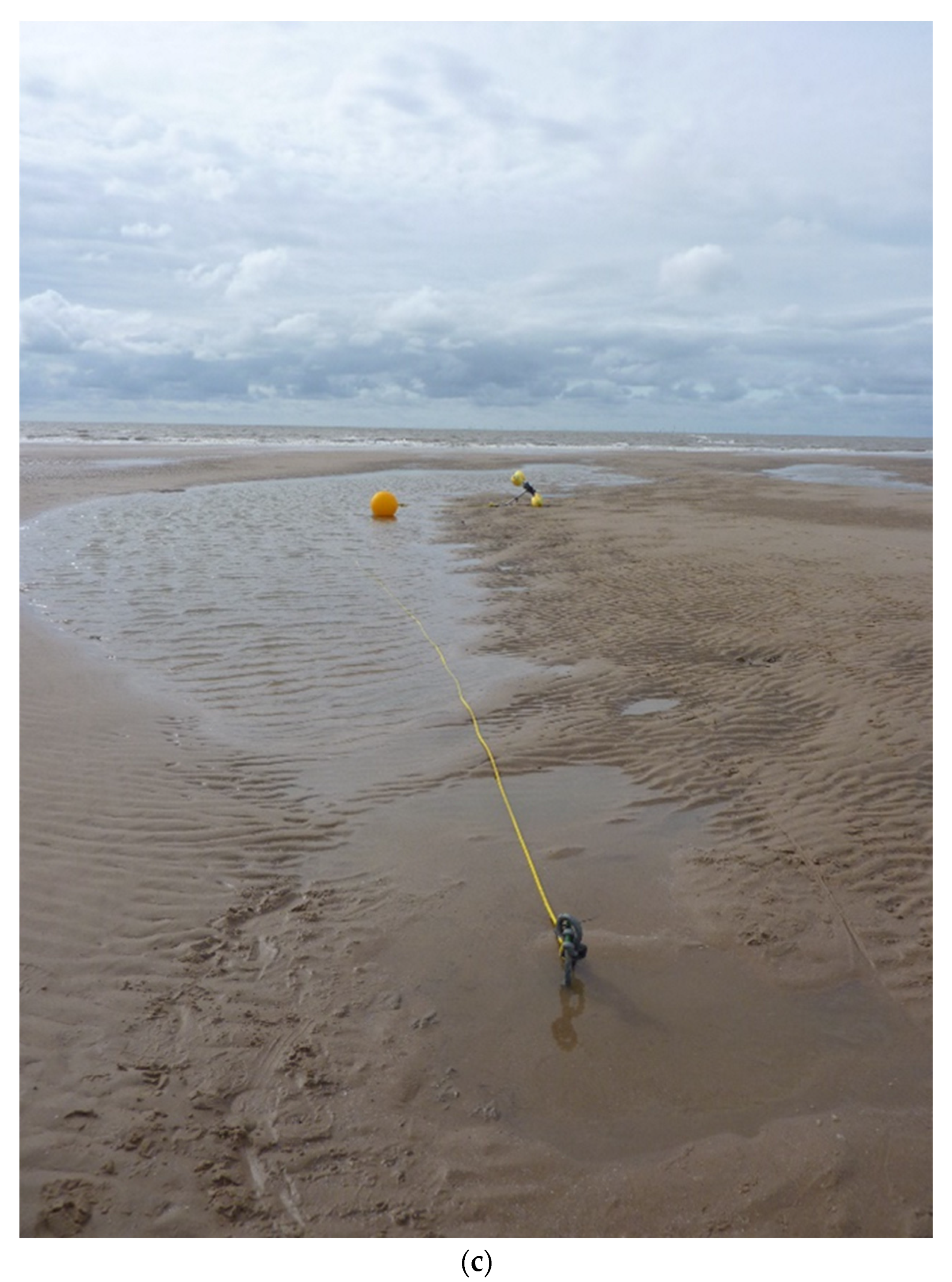
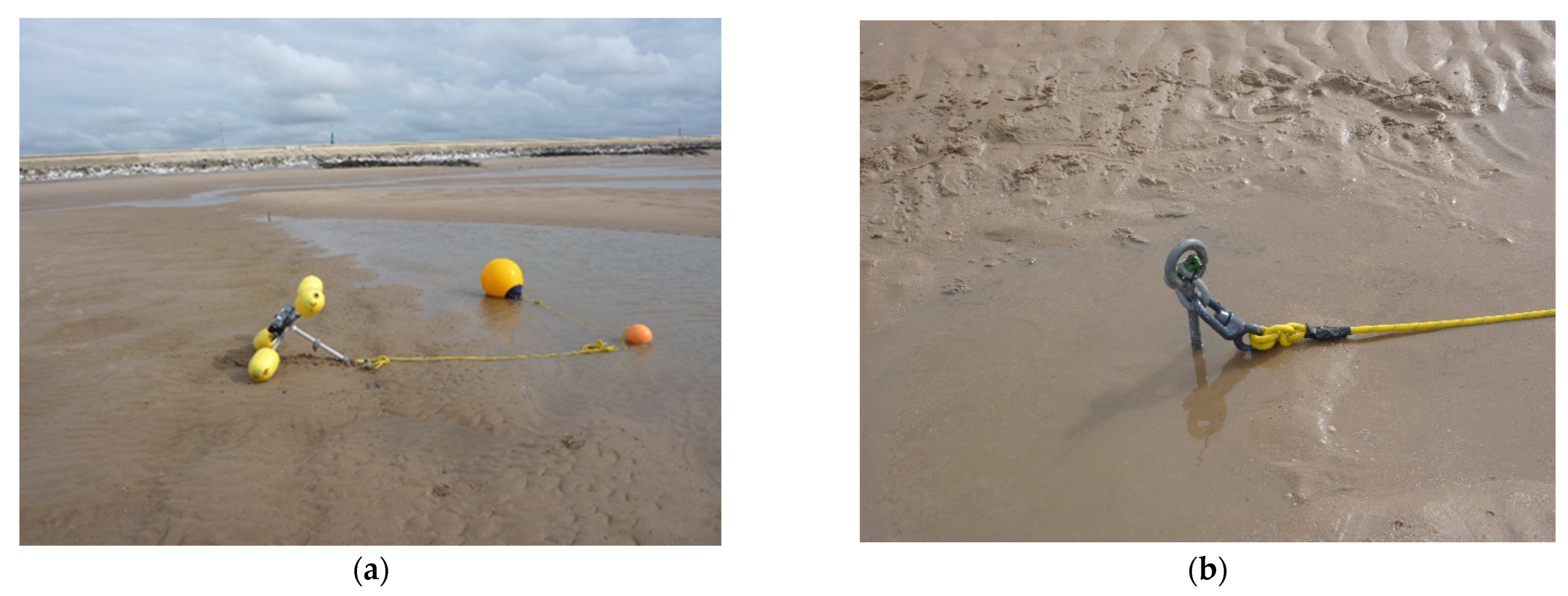
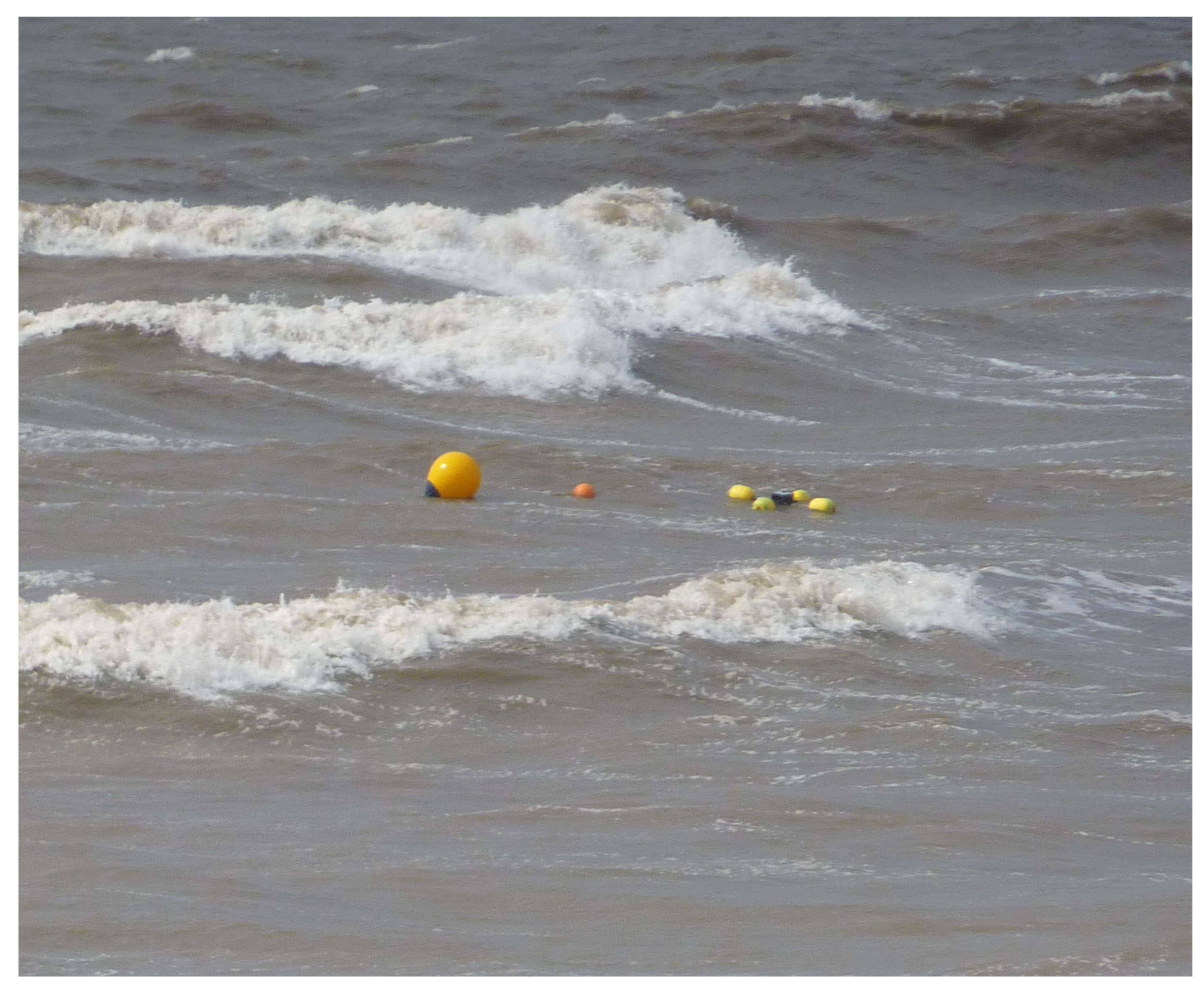
2.1. GNSS Buoy Set-Up and Mooring Design

Our GNSS buoy configuration was the same as that used at Holyhead harbour [8], with the GNSS antenna, receiver and battery attached to the top of the platform and secured between the yellow trawl floats (Figure 1a). The overall cost was around USD 400 (buoy parts USD 140, GPS/logger USD 260; all buoy parts sourced from suppliers in the UK, GPS/logger sourced from Emlid Reach [19]). The GNSS system consisted of a U-blox M8T [20] single frequency receiver (embedded on the Emlid Reach [19]) using a Tallysman patch antenna, with a 10 cm square aluminium ground plane. The ground plane is essential to reduce multi-path reflections and increase the antenna gain [21]; its optimum dimensions (often supplied with antenna manufacturer’s specifications) are determined by the antenna size. An EasyAcc 20,000 mAh battery pack was used with the Emlid Reach, which provided enough power to cover the period of the experiment; the expected endurance based on the power requirements is up to 4 days. The Emlid Reach was also Wi-Fi-enabled, and this is the method used for downloading data to a laptop after the deployment (typically ~100 Mb of zipped raw U-blox format data per day). In trials with an Alpha network antenna (AC1200 USB Wireless Adapter) connected to a laptop, a distance of up to 500 m was achieved for successful downloads with the mooring still floating in the water (without needing to recover, and open the electronics enclosure).

GPS and GLONASS raw satellite data were recorded at 5 Hz, including the carrier phase information in the U-blox binary format (ubx). To reduce the chance of water ingress into the electronics box, cable ties were applied around the lid to provide additional support to the clamped lid-closure catch.

To allow for more free movement of the buoy, the mooring used two additional surface floats (Figure 1a), with the GNSS buoy attached directly to a small Gael Force trawl float and then to a larger yellow polyform A3 buoy. This mooring set-up allows the GNSS buoy to float on the horizonal water level and reduces any angled inclination towards the anchor point. Figure 1a shows the top part of the mooring with the GNSS buoy, trawl float and polyform buoy (~5 m of rope between the GNSS buoy and the polyform buoy). Small 200 g weights were attached to the middle sections of each rope segment to keep the connections under water and to reduce the chance of tangling with the GNSS buoy float arms. Figure 1b shows the 15 m of rope connected to the ground anchor (1 m in length) which was screwed into the sand (the swivel helps to prevent the main mooring line from twisting). Figure 1c shows the two different parts of the mooring connected together on the beach at low water.

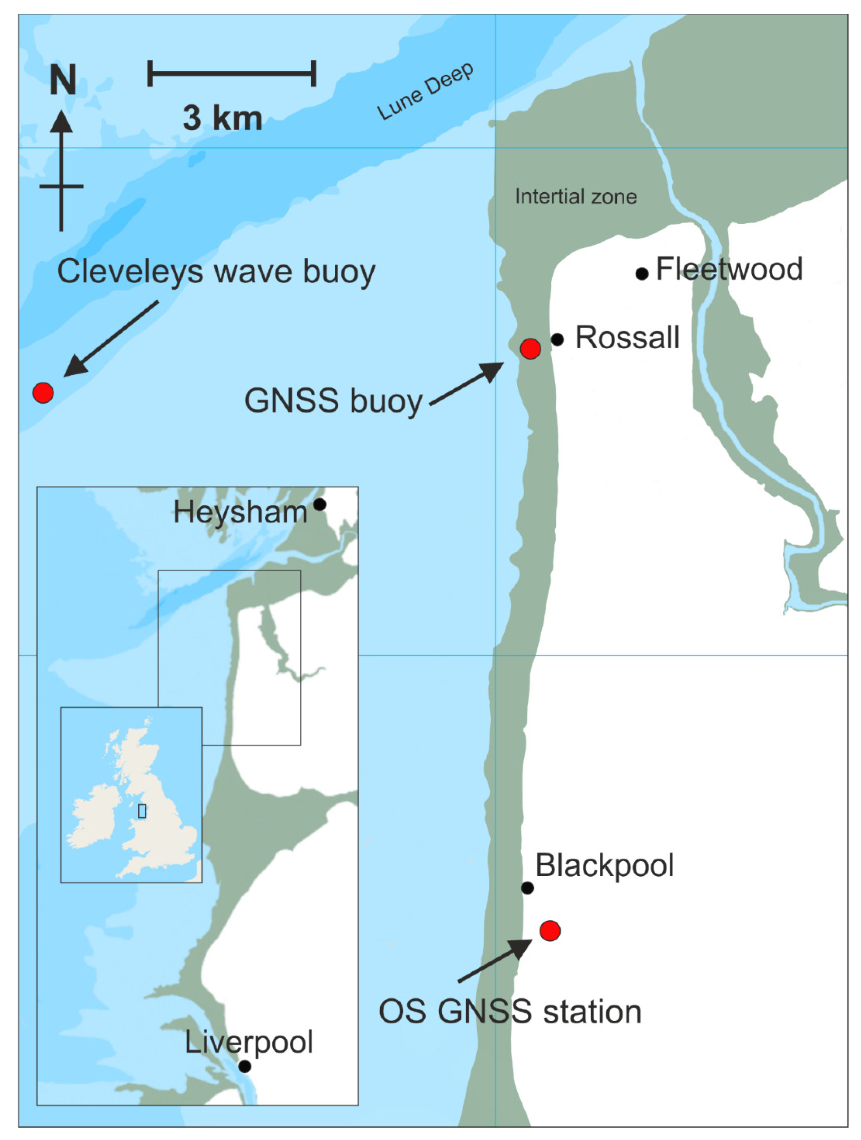
2.2. Buoy Testing at Rossall

Rossall, near Fleetwood in NW England, (Figure 2) was chosen for the beach deployment. This location is macro-tidal and has dissipative beach characteristics [22,23] because it consists of fine sand, has a gentle profile gradient (e.g., 1:50), and has a medium intertidal zone (~300 m). It is likely that spilling waves would be present, which typically dissipate their energy gradually over a wide surf zone. The location of the GNSS buoy was adjacent to an existing coastal monitoring system (consisting of a deployed X-band radar), and would provide a realistic ‘typical’ setting for an assessment of its capability.

The buoy was attached to the ground anchor (Figure 1b) and laid flat on the beach (deployed position: WGS: 53°54′48.6″ N, 03°03′14.3″ W). It was approximately 250 m from the foot of the concrete sea defences, and between two rock armour groynes that are perpendicular to the sea defences and around 100 m in length. The returned sea level and wave data indicate that a semi-permanent deployment of this GNSS buoy would provide the necessary data for analysis of X-band radar data, which would in turn improve the accuracy of the derived spatial and temporal beach morphology [1].

2.3. Local Tide and Storm Surge Data

Tidal data for comparison with the GNSS buoy results were obtained from the UK Environment Agency (EA) tide gauges at Liverpool (WGS: 53°26′58.9″ N, 03°01′5.2″ W, British National Grid: SJ 3248 9525) 50 km to the south, and Heysham (WGS: 54°01′54.5″ N, 02°55′13.4″ W, British National Grid: SD 3982 5993) 15 km to the north-east, downloaded from British Oceanographic Data Centre (BODC) website www.bodc.ac.uk (accessed on 4 June 2021). The EA tidal data were recorded as 15 min averages; the EA gauges are part of the UK National Tide Gauge Network [24]. Both of these tide gauges are full-tide bubbler tide gauge systems [25]. The datum used throughout is local chart datum (CD), which at Rossall is 4.90 m below Ordnance Datum Newlyn (ODN).

Tidal predictions of high water (HW) and low water (LW) [26] are shown in

Table 1. Tidal predictions for Liverpool (Gladstone Lock), Blackpool and Heysham (from POLTIPS 2009) for 28–29 August 2019.

	Liverpool		Blackpool		Heysham
	Time	Ht (m)	Time	Ht (m)	Time	Ht (m)
Wed 28 August	15:52	2.00 LW	15:38	2.17 LW	15:51	1.97 LW
	21:32	8.92 HW	21:23	8.87 HW	21:42	9.10 HW
Thu 29 August	04:30	1.49 LW	04:14	1.60 LW	04:29	1.49 LW
	10:00	9.12 HW	09:55	9.01 HW	10:11	9.33 HW
	16:48	1.49 LW	16:32	1.61 LW	16:45	1.49 LW

. At Blackpool, high water was predicted to be 8.87 m at 21:23 on 28 August 2019 and 9.01 m at 10:42 on 29 August. The highest predicted tide of the spring cycle was 10.27 m on 2 September at 12:64; hence, the tides during the experiment were close to the peak springs. Tide gauge data at Liverpool and Heysham show that leading up to these high waters, the storm surge heights were relatively small: ~0.1 m for the first tidal cycle and ~0.3 m for the second tidal cycle [27].

2.4. Offshore Wave Data

Wave data, for comparison with the GNSS buoy data, were obtained (via the Channel Coastal Observatory website https://coastalmonitoring.org/ (accessed on 4 June 2021)), from the Cleveleys wave buoy (WGS: 53°53.70′ N, 03°11.78′ W) owned by Sefton Council and situated 9.5 km to the west (Figure 2) of the GNSS deployment site at Rossall. The wave data were recorded as thirty-minute values by the Datawell Directional Waverider Mk III buoy deployed in approximately 10 m of water depth. For reference, and to contrast with the wave heights encountered during the experiment in August 2019, the mean significant wave height (Hs) was 1.0 m, and standard deviation was 0.60 m, with minimum value of 0.09 m and maximum value of 2.67 m.

2.5. GNSS Base Station and Satellite Ephemerides Data

There is a UK Ordnance Survey (OS) geodetic GNSS site located at Blackpool airport (WGS: 53°46′36.9″ N, 03°02′05.9″ W, British National Grid: SD 31891 31673), 14.5 km to the south of the deployment site; a source of research-quality GNSS data which can be applied to the post-processed kinematic (PPK) solution. Initial processing used base station data at 30 s intervals from the Ordnance Survey. Once the 1 Hz data became available (after a delay of 45 days) these were used in the final positioning solution instead. The archived 1 Hz GNSS data were obtained from the British Isles continuous GNSS facility (BIGF) [28].

To improve the overall solution, satellite ephemerides for precise orbit corrections and satellite and station clock error corrections were applied. These were obtained from the Crustal Dynamics Data Information System [29,30]. The corrections are delivered with increasing accuracy in the form of ‘ultra’, ‘rapid’ and ‘final’ correction files; available between 3–9 h, 17–41 h and 11–17 days, respectively. The results in this paper use the final products.

3. Results and Interpretation

The raw data were downloaded via Wi-Fi using the set-up mentioned in Section 2.1; this was tested at around 250 m range to demonstrate that data could be downloaded with the buoy in the water. If deployed further out towards the low water mark it could be free-floating at times during the spring-neap tidal cycle (e.g., during neap tidal cycles). Data were recorded from 14:10 on 28 August until 15:25 on 29 August over two tidal cycles. The data were subdivided according to when the buoy was free-floating during the tidal cycle such that:

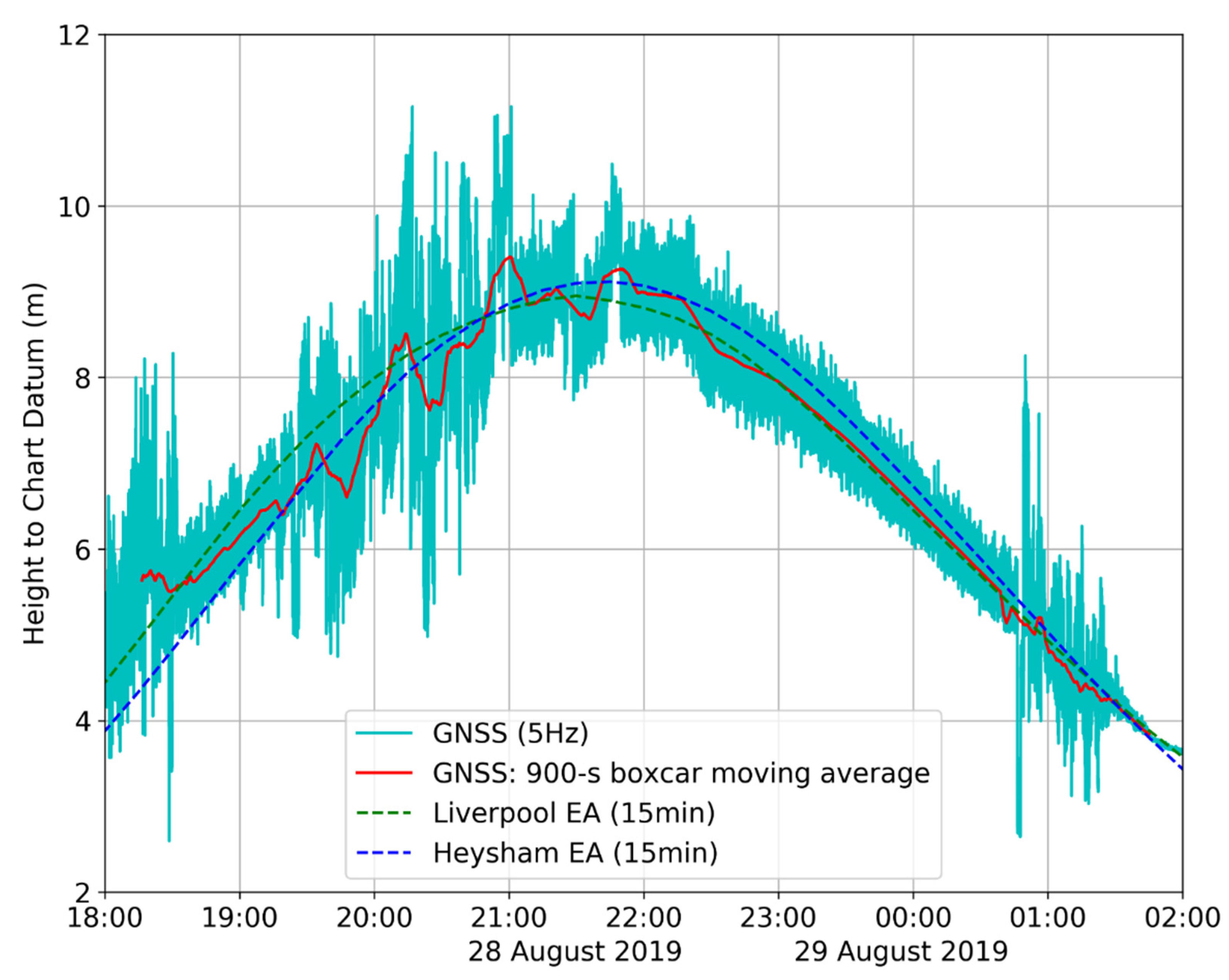
• tidal cycle A refers to data between 18:00 on the 28 August 02:00 on the 29 August.
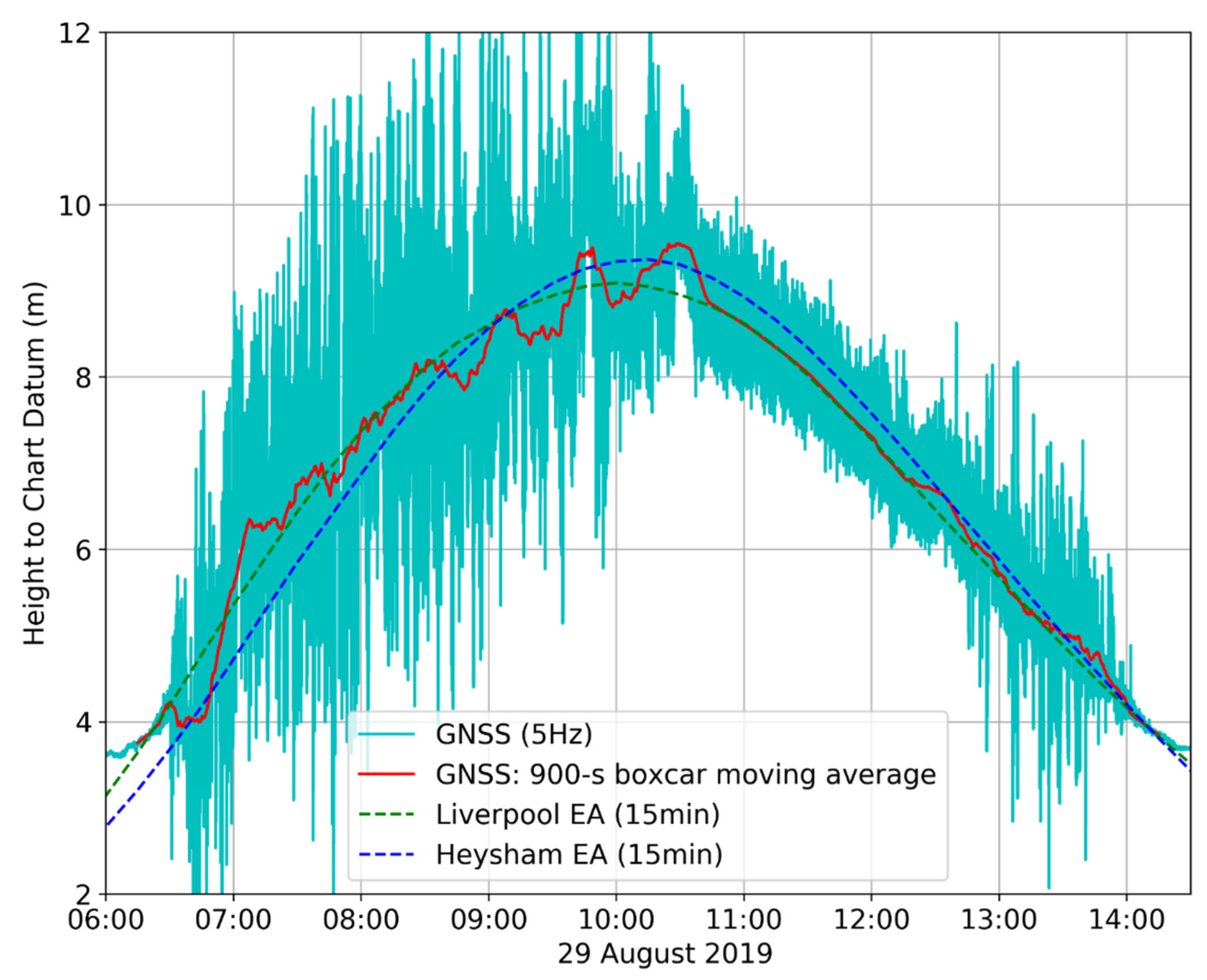
• tidal cycle B refers to data between 06:00–14:30 on the 29 August.

3.1. GNSS-Derived Tidal Heights

The RTKLIB software [5] has a number of options for post-processing GNSS data.

Table 2. Parameter settings for the post-processing using RTKLIB.

Parameter	Value
Solution	Kinematic
Frequency	L1
Sensor dynamics	On
Earth tides	Off
Ionosphere	Broadcast
Troposphere	Saastamoinen
Ephemerides	Precise
Satellite system	GPS + GLONASS
Ambiguities GPS	Fix & Hold
Ambiguities GLONASS	On

shows the general settings that produced the best overall solutions. GNSS data from GPS and global navigation satellite system (GLONASS) satellites were post-processed in ‘kinematic mode’ with respect to a land-based reference station. Post-processed kinematic (PPK) mode is an alternative technique to real-time kinematic (RTK) and differs in that the solution algorithms can be applied both forward and backward (to increase the accuracy of the overall solution) and more accurate timing corrections can be applied later. In addition, the elevation mask was set to 15° above the horizon (i.e., only using satellite data with angles from horizon greater or equal to 15°). The difference to a previous set-up [8] was to allow the RTKLIB software to use the GLONASS data to resolve ambiguities; this did slightly improve the results with ~5% more fixed solutions.

To produce centimetre-accurate solutions, the RTKLIB software uses both the code phase and, in particular, the carrier phase satellite data recorded by the base (static GNSS site at Blackpool) and rover (GNSS buoy) receivers. The software processes the data with an algorithm to determine the exact number of radio wavelengths between the satellites and the base station antenna (a method known as ‘ambiguity resolution’) and yield either a fixed or float solution. In a fixed solution (referred to as Q = 1, this is generally an indicator of a more accurate positional result), the number of wavelengths is a whole number, or integer, and the algorithm is constrained to yield a whole number. A low number of visible satellites, poor satellite constellation geometry, and distance between the rover and the base station is likely to prevent a fixed solution. If the algorithm does not yield an acceptable fixed solution, then the ambiguity is allowed to be a decimal or floating-point number and the solution is known as a float solution (Q = 2). Generally, results with Q1 solutions should indicate more accurate positional data than Q2 solutions.

Poorer solutions are often due to cycle slips which occur when the GNSS receiver loses its lock with a satellite; this results in a miss count of carrier phase cycles. These are more likely to occur when the receiver is moving, such as on the GNSS buoy with its horizontal and vertical movements. Cycle slips can be caused by obstructions, high accelerations, reflections, vibration or lack of a suitable antenna ground plane. Once the cycle count is lost the phase-bias estimate (within the RTKLIB software) must be reset and re-converged and this can take up to a minute or longer to recover.

The satellite data recorded in Rinex format from both the rover and base stations were processed in two parts, covering tidal cycle A and tidal cycle B, respectively.

Table 3. Percentage of fixed and float solutions.

	Fixed Q1%	Float Q2%
Tidal cycle A	57.0	43.0
Tidal cycle B	48.4	51.6

shows the percentage of fixed to float solutions. Q1 percentages shown in Table 3, ranging from 48.4% to 57.0%, indicate that at times during the deployment the GNSS receiver on the buoy was being affected by one or more of the conditions mentioned above. In contrast, the same GNSS buoy was used in a previous deployment in a relatively sheltered part of the harbour at Holyhead [8] and obtained almost 100% of Q1 solutions. Therefore, to further explore the cause of these lower Q1 percentages, the track (East–West versus North–South), individual positional components (North–South, East–West and Up–Down) and vertical accelerations for tidal cycle A and tidal cycle B are plotted in Figure 3, Figure 4, Figure 5, Figure 6, Figure 7 and Figure 8 respectively (Q1 solutions are shown in green, and Q2 solutions shown in orange).

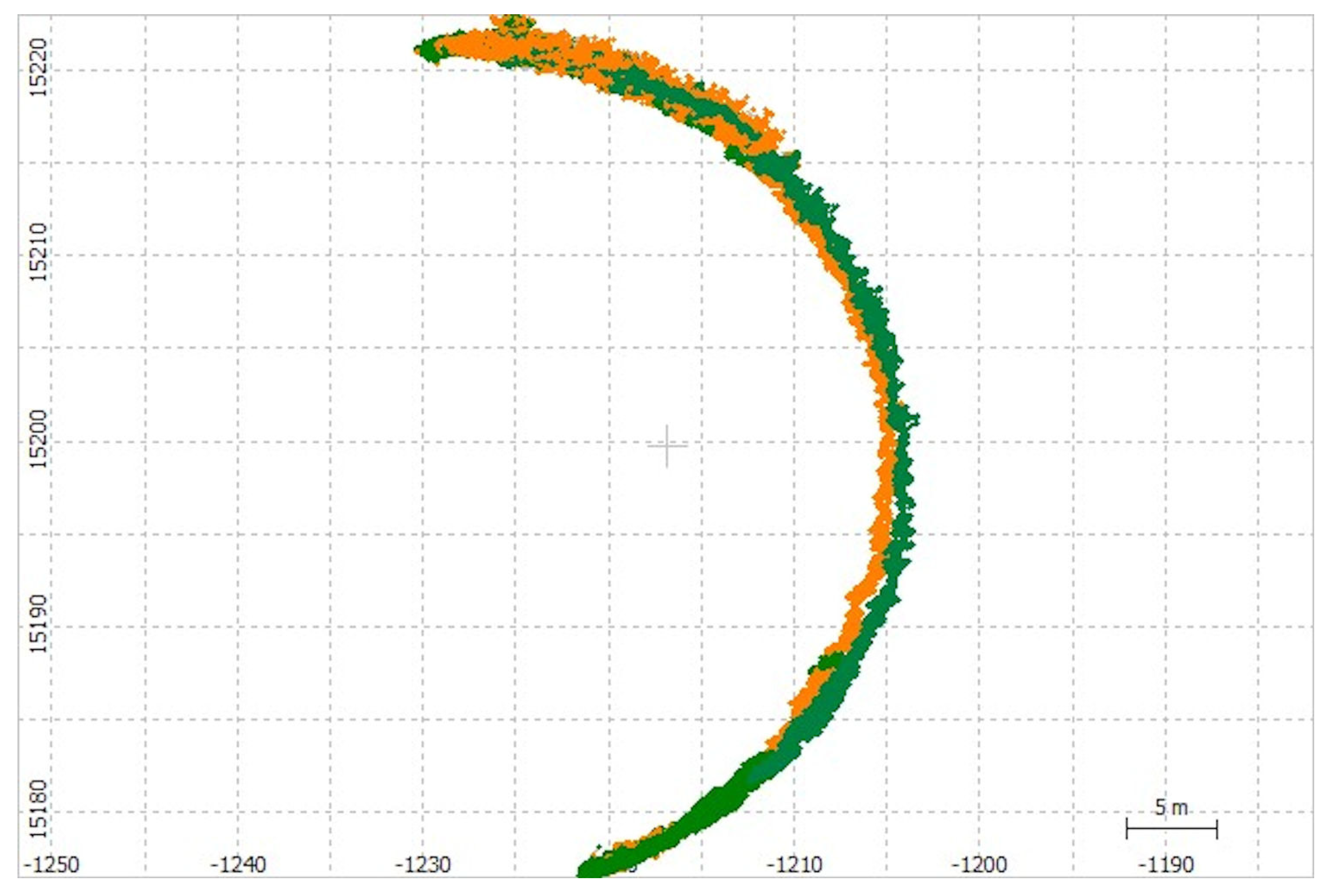
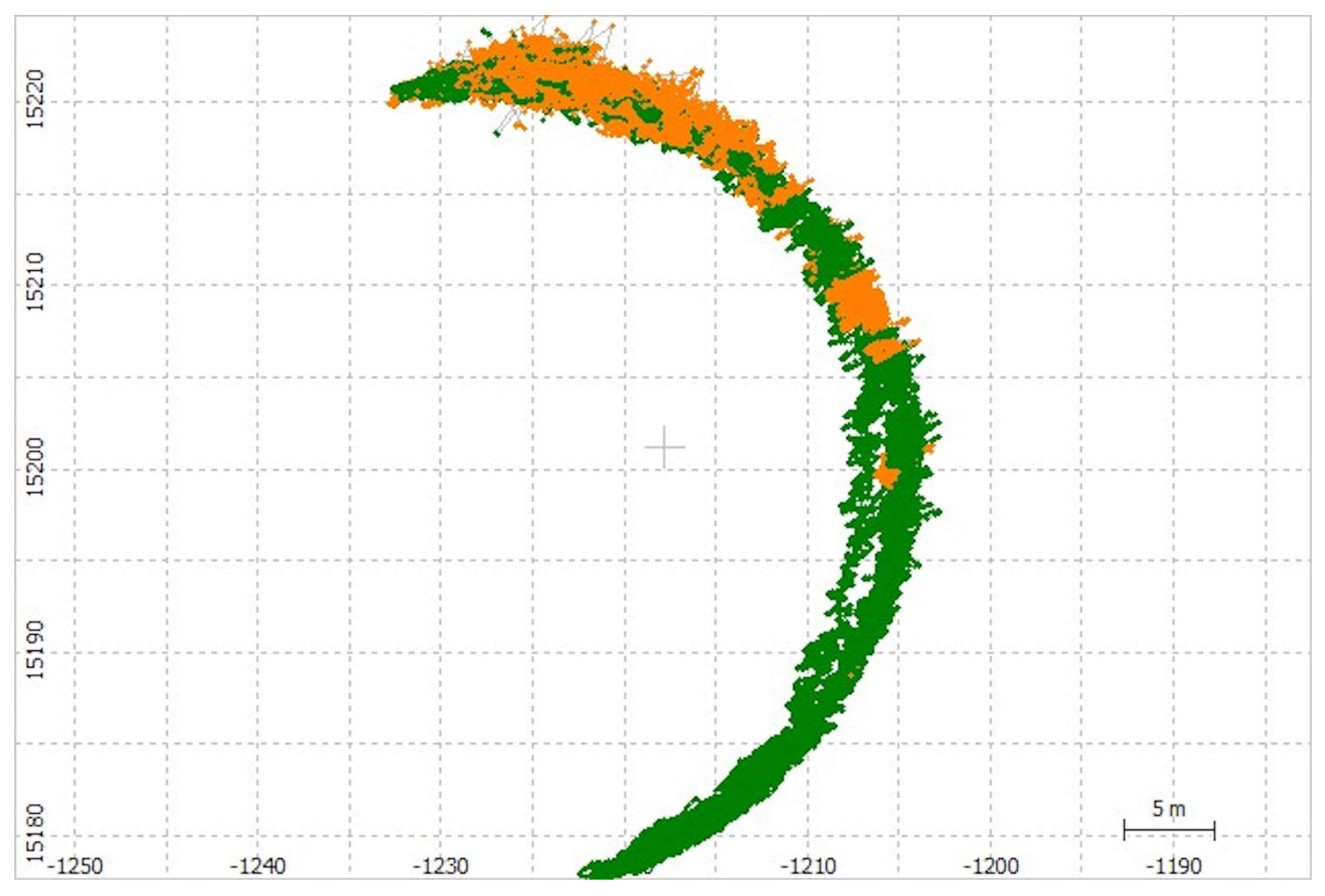
3.2. GNSS Buoy Track

The buoy tracks during tidal cycles A and B (Figure 3 and Figure 4, respectively) each display a rotational movement around the anchor point. There is a consistent northerly component during both flood tides (tidal cycle A 18:00–21:30, tidal cycle B 06:30–10:30) with a small increasing component towards the shore suggesting strong alongshore currents during the flood tide. During tidal cycle A, there was a consistent moderate breeze (11–15 knots) from the west; during tidal cycle B, there was an increasing fresh breeze (17–21 knots) from the south-west. The weather conditions also would have contributed to the dominant northerly orientation during the flood tide.

Shortly after high water in tidal cycle A, the rotation increases clockwise towards the shoreline, with its closest position to the shore being around 22:00, around 90 min after high water. It then continues to rotate clockwise until 23:00 when it then begins an anti-clockwise rotation passing the same position around 00:30. A similar pattern can also be seen with tidal cycle B. This could indicate water recirculation as tidal currents decrease, and being constrained by the short length (~100 m) rock groynes both to the north and south of the site. It is interesting to note that the majority of good consistent solutions (Q1) occurred shortly after high water and during the ebb tide, while the poorer solutions (Q2) occurred during the flood tide.

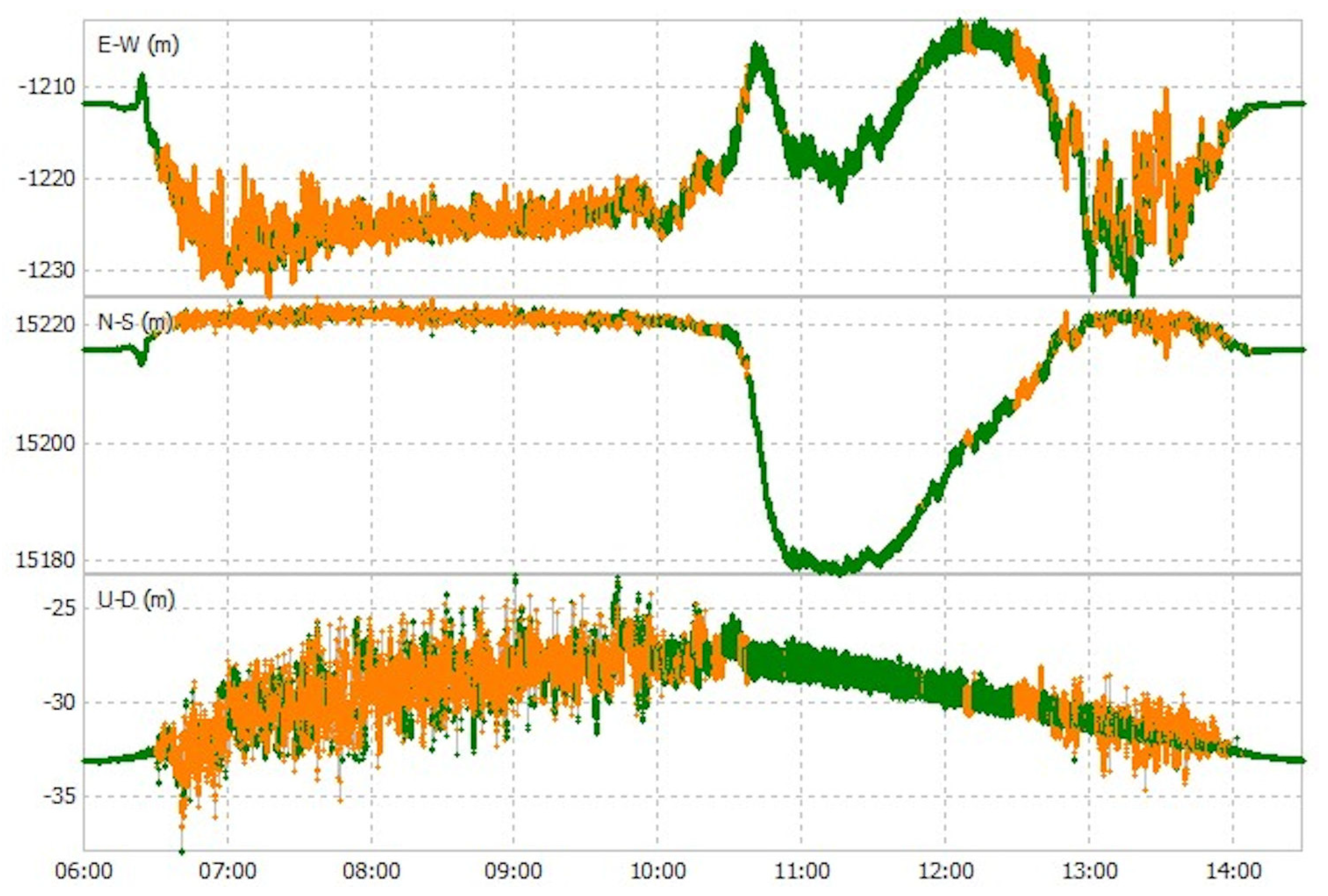
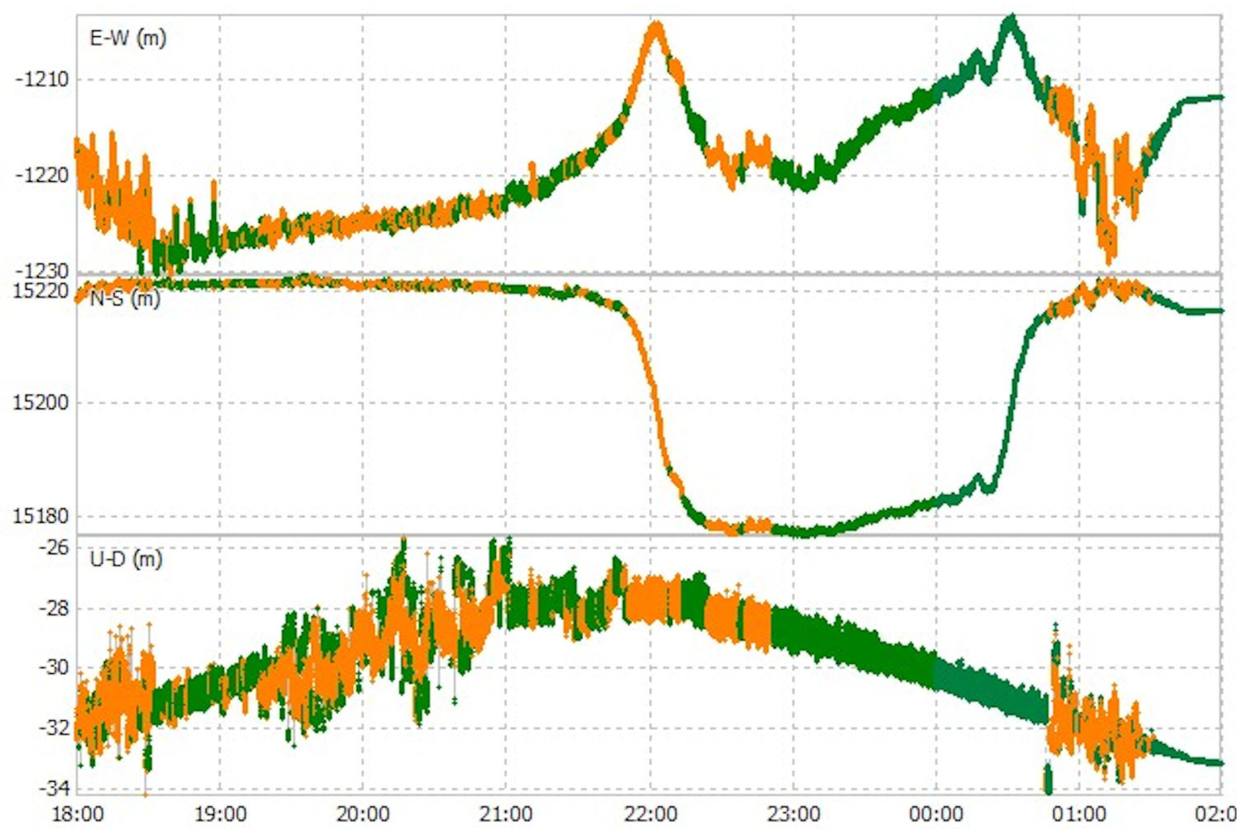
3.3. GNSS Buoy Positional Components

The buoy’s positional components during tidal cycles A and B are shown in Figure 5 and Figure 6, with East–West (E-W), North–South (N-S) and Up–Down (U-D) components. The poorest (Q2) solutions occurred more frequently during each flood tide: at maximum tidal current and on the approach towards high water. In addition, it is likely that the poor solutions at the start and end of both tidal cycles A and B were caused by the buoy being buffeted by small waves before becoming free-floating, i.e., with the central vertical bar catching the sand as the buoy moved with the small breaking waves.

The poorest Q2 solutions occurred during each flood tide and when the buoy was within the surf zone, and being affected by spilling waves. The buoy tracks (Figure 3 and Figure 4) suggest that the mooring line was under tension during the peak tidal flows on the flood tide, which may indicate the presence of relatively strong alongshore currents. When coincident with spilling waves this would briefly allow water to cover the antenna, resulting in loss of satellite lock; this type of effect can be seen clearly within the sea-level data.

Some Q1 solutions were obviously erroneous with large jumps (e.g., Figure 5, U-D~00:45 29 August). This was likely due to the processing software not recovering from poor and limited satellite data, and the subsequent offset feeding into the following positional solutions; therefore, Q1 solutions are not always an indication of good sea-level data.

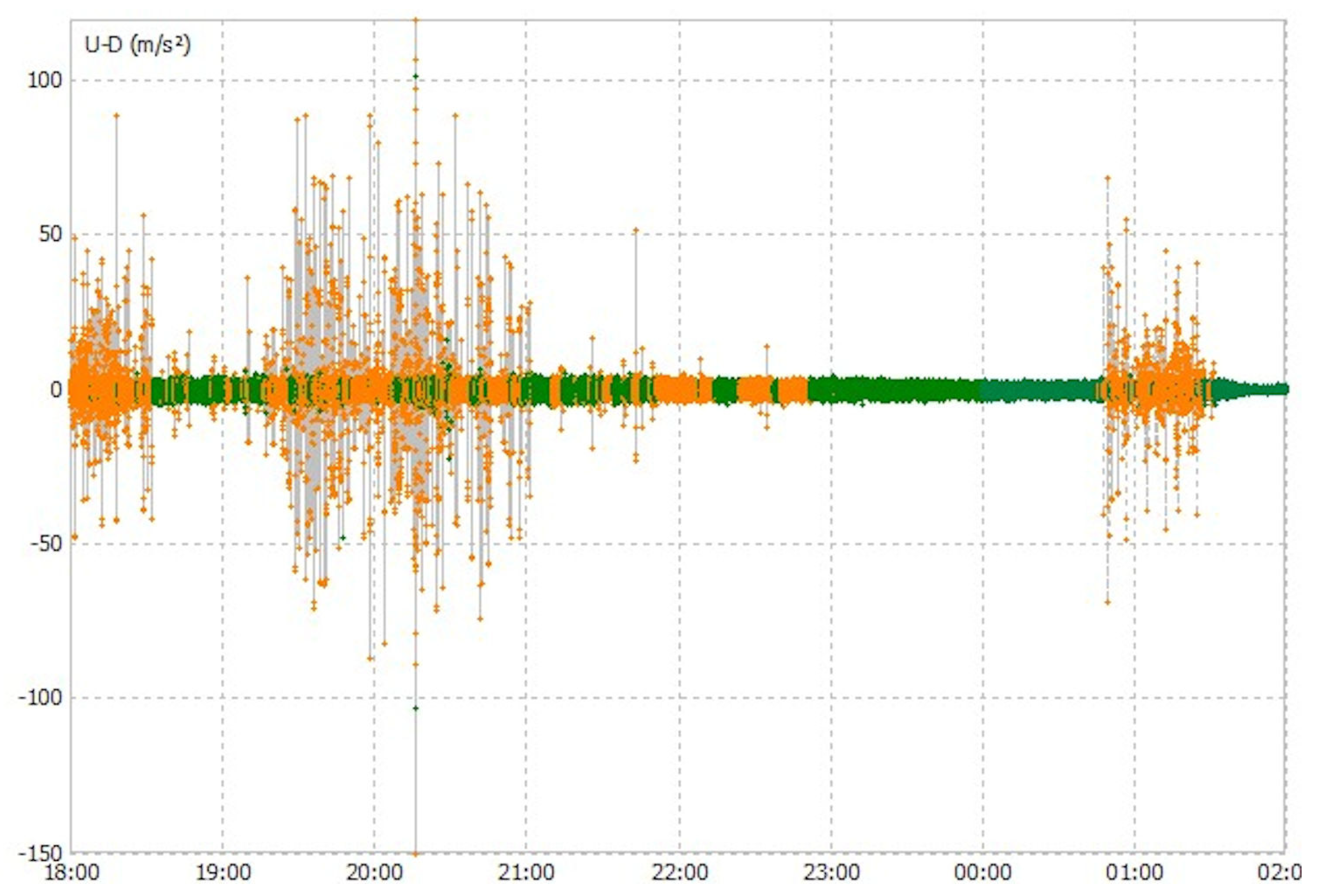
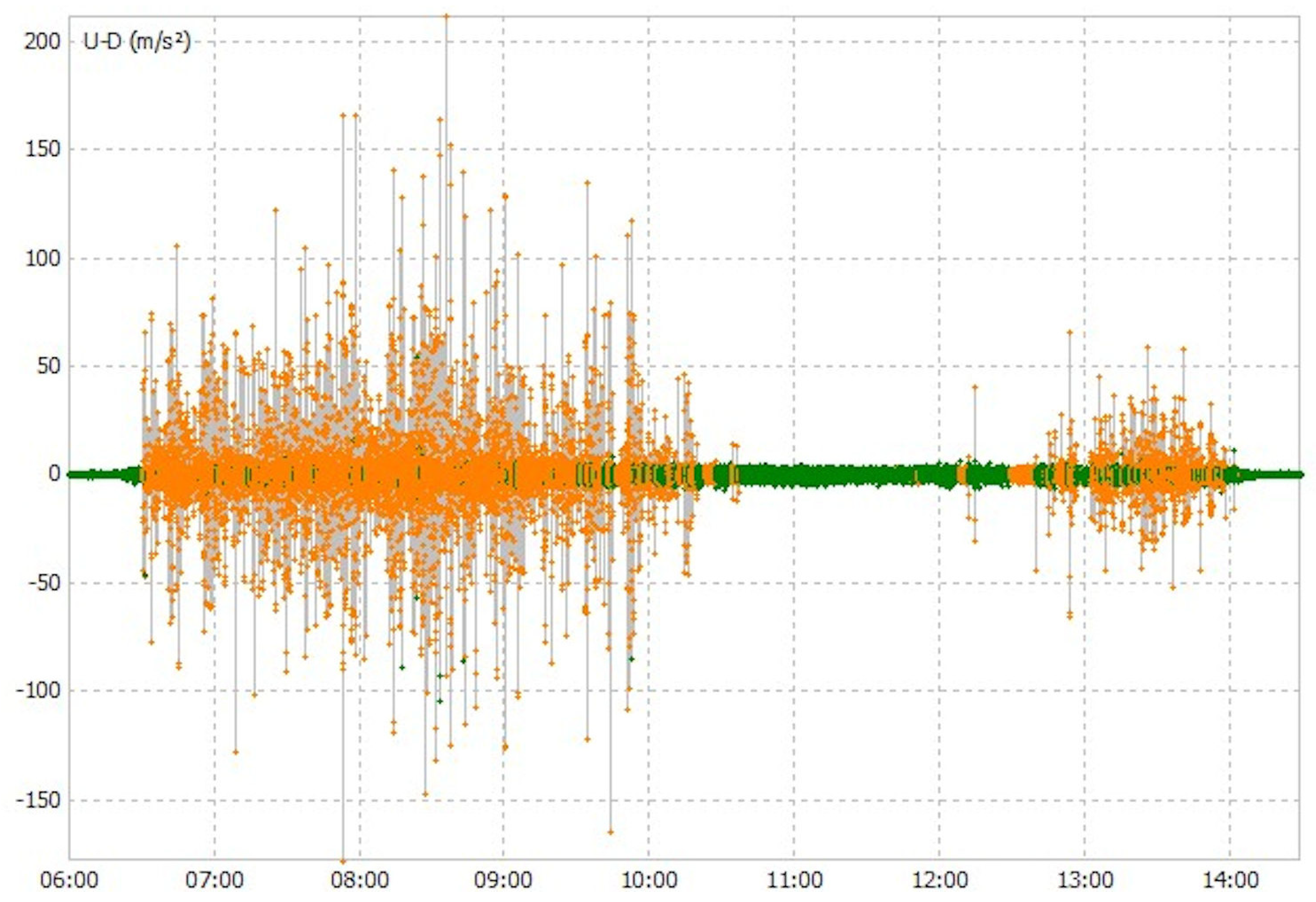
3.4. GNSS Buoy Vertical Accelerations

Most of the poor solutions, with the greatest vertical differences, coincide with very large accelerations (Figure 7 and Figure 8), mainly during the flood tides and when the buoy is in shallower water. When large accelerations occurred, the GNSS receiver Rinex data also indicated loss of satellite lock for the majority of visible satellites. Normal practice to improve the analysis when this happens is to experiment with increasing the satellite angle cut off, e.g., 16°, 17°, 18°, etc., ignoring any data with lower satellite angles. Unfortunately, this did not improve the solutions because the lock problem occurred simultaneously on all the satellites. In fact, it produced progressively poorer solutions due to smaller numbers of useable satellites for the RTKLIB software. It is likely that these poor solutions occur when the antenna is becoming covered in water from spilling waves, which were observed on a number of occasions from the shore; the mooring could be seen to be physically jerked backwards as the wave passed through. For example, the GNSS buoy (photograph in Figure 9) prior to recovery on the 29 August at 13:24: large accelerations were observed in the satellite data (Figure 8). In this case, white water was seen behind the buoy and it eventually washed over it and this coincided with the high recorded accelerations and loss of satellite lock, and thus a poor positional solution.

4. Analysis and Discussion

4.1. Buoy Performance

On recovery, there were a number of twists in the rope connection between the GNSS buoy and the trawl float. An additional swivel on the end of the GNSS buoy connection would probably have reduced this and may lead to a more stable and free-floating platform. The use of a rubber bungee directly below the wave buoy mooring [18] may be worth incorporating in this mooring in future. Both these suggestions may allow more free movement in the strong alongshore currents during the flood tide and thus improve data quality. In addition, the anchor point was completely covered with about 0.25 m of sand over just a couple of tidal cycles, so the bottom swivel was probably not working as intended by the end of this period. Overall, the mooring arrangement appears to have worked well and coped without being damaged in a very dynamic part of the intertidal beach. If the deployment was further away from the sea defences and nearer the low water mark, then spilling waves may have less impact on the results due to spending less time in the surf zone. Other authors observed the reverse [18] since they had to site their mooring closer to shore so as to pick up the breaking/spilling waves.

4.2. GNSS Receiver Performance

Instead of a single frequency (L1) receiver, a dual frequency (L1, L2) receiver could be substituted and this would improve accuracy by providing more data (i.e., signals from twice as many satellite) for processing by the RTKLIB software. Since this experiment was conducted, Emlid Reach have produced an upgrade to the receiver for a similar cost (e.g., using a F9 Ublox dual frequency GNSS receiver). It also supplies a helix antenna, an improvement on the patch antenna; its larger design would reduce the problem with spilling waves, and be less susceptible to reflections (which increase the signal to noise ratio). Use of a duplicate set-up for both rover and base station, both recording at 5 Hz (in this experiment, the base station was recording at 1 Hz) would eliminate problems associated with unknown antenna bias (with the patch antenna) [8], and would allow additional options in the RTLKLIB software to be used, which would then likely improve the position solutions.

4.3. Sea Levels

Derived tidal heights relative to chart datum for tidal cycle A are shown in Figure 10, whereas Figure 11 shows the corresponding results for tidal cycle B. Tide gauge data from Liverpool and Heysham are added for comparison with those obtained from the GNSS buoy. A 15 min (900 s ‘boxcar’) moving average was applied to the buoy data before comparison with the 15 min Liverpool and Heysham tide gauge data. Both Figure 10 and Figure 11 emphasise the periods of good data during the ebb tide (e.g., comparison with GNSS 900 s average and Liverpool 15 min data; mean difference −0.02 m, standard deviation difference 0.03 m and RMSE difference 0.04 m) and poorer data during the flood tide. Although the tidal characteristics between Liverpool, Heysham and Rossall are similar, there are small but significant differences in the tidal elevations and times of LW and HW (Table 1); thus, these comparisons are considered indicative of data quality, i.e., good data quality during the ebb periods.

During the ebb tide the 15 min GNSS buoy data matches the Liverpool tide gauge data more closely in both timing and elevation, even though the Heysham tide gauge is nearer. The larger differences between the GNSS buoy and the Heysham tide gauge data are probably due to Heysham being at the edge of Morecambe Bay (with the accompanying dynamics of a larger intertidal zone, and the water being initially directed along the Lune Deep channel at low water). However, on the ebb tide there are some good data between 18:30 and 19:30 on 28 August (Figure 10), which indicate timing differences compared with the Liverpool tidal data. Again, both Figure 10 and Figure 11 show there are poorer data as the water at the buoy approaches ‘drying out’.

This low cost GNSS buoy is suitable for providing sea-level (and wave) data to support X-band radar monitoring systems of coastal morphology changes over time scales from days to years. During the tidal cycle, the radar system records the advancing and retreating shorelines (using the water-line method [1]) which are then assigned altitudes based on corresponding water-levels from a local tide gauge. Previous research [1] indicates that the accuracy of the beach-derived morphology maps is greatly improved if tidal measurements are available within the radar footprint.

4.4. Wave Characteristics

The power spectral density of GNSS buoy tidal elevations (Figure 12) show that for tidal cycle A, the resultant peak frequency corresponds to a wave period of 5.3 s, whereas tidal cycle B has a peak frequency corresponding to a wave period of 5.1 s.

Figure 13a–d shows the power spectral density results from the Cleveleys wave buoy over two-hour periods before and after high water for comparison with the GNSS buoy (see

Table 4. Wave parameter comparisons between the GNSS buoy and the Cleveleys wave buoy for two-hour periods either side of high water (HW).

		Significant Wave Height		Spectral Peak Period
		GNSS Buoy	Cleveleys Buoy	GNSS Buoy	Cleveleys Buoy
Tidal cycle A	2 hr period before HW	1.1 m	0.9 m	4.8 s	5.0 s
	2 hr period after HW	1.0 m	1.0 m	5.0 s	4.8 s
Tidal cycle B	2 hr period before HW	1.5 m	1.5 m	4.7 s	4.8 s
	2 hr period after HW	1.3 m	1.6 m	5.4 s	5.3 s

). The significant wave heights were estimated by calculating four times the square root of the area from under the peak of spectral density [11] between the frequency bands 0.5 and 0.125 Hz.

The GNSS buoy results compare well with the Cleveleys wave buoy data, giving similar significant wave heights and spectral peak periods. Significant wave height differences vary between 0.0 and 0.3 m; however, in general they are a very close match and indicate that the GNSS buoy is capable of measuring waves as well as a commercial wave buoy. Differences in spectral peak periods within 0.1 s are also very similar. The results here also indicate that wave heights and wave periods increased over the two tidal cycles, and this can also be seen in the sea level data variations (Figure 10 and Figure 11).

5. Conclusions

The GNSS buoy recorded data in very challenging conditions and provided both sea-level and wave data. These GNSS data show that the tidal elevations are a closer match to tide gauge data at Liverpool than at Heysham, although there may be subtle differences especially during the flood tide; however, during the ebb periods the comparison with GNSS 900 s average and Liverpool 15 min data produced a mean difference −0.02 m, standard deviation difference 0.03 m and RMSE difference 0.04 m. In addition, the GNSS buoy recorded almost indistinguishable significant wave heights (differences between 0.0 and 0.3 m; Table 4) and wave periods (differences between 0.1 and 0.2 s; Table 4) to those measured by the Cleveleys wave buoy. It was possible to extract wave data from the poorer positional solutions during the flood tide and when there were large accelerations in the GNSS buoy.

Overall, the deployment over two tidal cycles showed that the GNSS buoy can perform within the intertidal zone, and provide acceptable sea-level and good quality wave data. In addition, it was demonstrated that these data can also be downloaded remotely which would allow for timely analysis. This approach offers considerable efficacy for determining local hydrodynamics in support of coastal monitoring or defence scheme implementation.

References

1. Bird, C.O.; Bell, P.S.; Plater, A.J. Application of marine radar to monitoring seasonal and event-based changes in intertidal morphology. Geomorphology 2017, 285, 1–15. [Google Scholar] [CrossRef] [Green Version]
2. Nicholls, R.J.; Wong, P.P.; Burkett, V.; Codignotto, J.; Hay, J.; McLean, R.; Ragoonaden, S.; Woodroffe, C.D.; Abuodha, P.; Arblaster, J. Coastal Systems and Low-Lying Areas. 2007. Available online: https://ro.uow.edu.au/scipapers/164 (accessed on 5 July 2021).
3. Spodar, A.; Héquette, A.; Ruz, M.-H.; Cartier, A.; Grégoire, P.; Sipka, V.; Forain, N. Evolution of a beach nourishment project using dredged sand from navigation channel, Dunkirk, northern France. J. Coast. Conserv. 2018, 22, 457–474. [Google Scholar] [CrossRef]
4. Habel, S.; Fletcher, C.H.; Barbee, M.; Anderson, T.R. The influence of seasonal patterns on a beach nourishment project in a complex reef environment. Coast. Eng. 2016, 116, 67–76. [Google Scholar] [CrossRef]
5. RTKLIB: An Open Source Program Package for GNSS Positioning. Available online: http://www.rtklib.com/ (accessed on 10 January 2019).
6. Pugh, D.; Woodworth, P. Sea-Level Science: Understanding Tides, Surges, Tsunamis and Mean Sea-Level Changes; Cambridge University Press: Cambridge, UK, 2014. [Google Scholar]
7. Williams, S.D.; Bell, P.S.; McCann, D.L.; Cooke, R.; Sams, C. Demonstrating the potential of low-cost GPS units for the remote measurement of tides and water levels using interferometric reflectometry. J. Atmos. Ocean. Technol. 2020, 37, 1925–1935. [Google Scholar] [CrossRef]
8. Knight, P.J.; Bird, C.O.; Sinclair, A.; Plater, A.J. A low-cost GNSS buoy platform for measuring coastal sea levels. Ocean. Eng. 2020, 203, 107198. [Google Scholar] [CrossRef]
9. André, G.; Míguez, B.M.; Ballu, V.; Testut, L.; Wöppelmann, G. Measuring sea level with GPS-equipped buoys: A multi-instruments experiment at Aix Island. Int. Hydrogr. Rev. 2013, 10, 27–38. [Google Scholar]
10. Stal, C.; Poppe, H.; Vandenbulcke, A.; De Wulf, A. Study of post-processed GNSS measurements for tidal analysis in the Belgian North Sea. Ocean. Eng. 2016, 118, 165–172. [Google Scholar] [CrossRef]
11. Fiorentino, L.A.; Heitsenrether, R.; Krug, W. Wave Measurements From Radar Tide Gauges. Front. Mar. Sci. 2019, 6, 586. [Google Scholar] [CrossRef]
12. Martins, K.; Blenkinsopp, C.E.; Power, H.E.; Bruder, B.; Puleo, J.A.; Bergsma, E.W. High-resolution monitoring of wave transformation in the surf zone using a LiDAR scanner array. Coast. Eng. 2017, 128, 37–43. [Google Scholar] [CrossRef]
13. Datawell, Directional Waverider MkIII, Brochure. Available online: https://www.datawell.nl/Portals/0/Documents/Brochures/datawell_brochure_dwr-mk3_b-09-09.pdf (accessed on 5 July 2021).
14. MacIsaac, C.; Naeth, S. TRIAXYS next wave II directional wave sensor the evolution of wave measurements. In Proceedings of the 2013 OCEANS-San Diego, San Diego, CA, USA, 23–27 September 2013; pp. 1–8. [Google Scholar]
15. Andrews, E.; Peach, L. An evaluation of current and emerging in-situ ocean wave monitoring technology. In Proceedings of the Australasian Coasts and Ports 2019 Conference: Future Directions from 40 [Degrees] S and Beyond, Hobart, Australia, 10–13 September 2019; p. 34. [Google Scholar]
16. Datawell, Mini Directional Waverider GPS. Available online: https://www.datawell.nl/Portals/0/Documents/Brochures/datawell_brochure_dwr-g4_b-06-10.pdf (accessed on 5 July 2021).
17. Spotter: The Agile Metocean Buoy. Available online: https://www.sofarocean.com/products/spotter (accessed on 5 July 2021).
18. Brown, A.C.; Paasch, R.K. The Accelerations of a Wave Measurement Buoy Impacted by Breaking Waves in the Surf Zone. J. Mar. Sci. Eng. 2021, 9, 214. [Google Scholar] [CrossRef]
19. Emlid Reach M+ RTK GNSS Module for Precise Navigation and UAV Mapping. Available online: https://emlid.com/ (accessed on 16 April 2019).
20. U-blox, Product Details for M8T Series GNSS Receivers. Available online: https://www.u-blox.com/en/product/neolea-m8t-series (accessed on 16 April 2019).
21. Ublox, Application Note: GPS Antennas, RF Design Considerations for U-blox GPS Receivers. Available online: https://www.u-blox.com/sites/default/files/products/documents/GPS-Antenna_AppNote_(GPS-X-08014).pdf (accessed on 24 May 2019).
22. Scott, T.; Masselink, G.; Russell, P. Morphodynamic characteristics and classification of beaches in England and Wales. Mar. Geol. 2011, 286, 1–20. [Google Scholar] [CrossRef] [Green Version]
23. Wright, L.D.; Short, A.D. Morphodynamic variability of surf zones and beaches: A synthesis. Mar. Geol. 1984, 56, 93–118. [Google Scholar] [CrossRef]
24. UK National Tide Gauge Network. Available online: https://www.bodc.ac.uk/data/hosted_data_systems/sea_level/uk_tide_gauge_network/ (accessed on 1 October 2019).
25. Woodworth, P.L.; Smith, D.E. A one year comparison of radar and bubbler tide gauges at Liverpool. Int. Hydrogr. Rev. 2003, 4, 42–49. [Google Scholar]
26. National Oceanography Centre POLTIPS-3: Coastal Tidal Software. Available online: http://noc.ac.uk/business/marine-data-products/coastal (accessed on 29 March 2020).
27. Archived Model Surge Outputs. Available online: https://www.ntslf.org/storm-surges (accessed on 19 April 2021).
28. NERC, British Isles Continuous GNSS Facility (BIGF). Available online: http://www.bigf.ac.uk/ (accessed on 3 May 2021).
29. CDDIS, NASA’s Archive of Space Geodesy Data. Available online: https://cddis.nasa.gov/Data_and_Derived_Products/GNSS/orbit_products.html (accessed on 18 April 2021).
30. Noll, C.E. The Crustal Dynamics Data Information System: A resource to support scientific analysis using space geodesy. Adv. Space Res. 2010, 45, 1421–1440. [Google Scholar] [CrossRef] [Green Version]
Figure 1. (a) Top part of mooring together with the GNSS buoy, (b) ground anchor with swivel, (c) complete mooring installed and laid out on the beach at low water.
Geosciences 11 00494 g001aGeosciences 11 00494 g001b
Figure 2. Location of Rossall experiment (Lancashire, UK); GNSS buoy, Ordnance Survey GNSS station, Cleveleys wave buoy. Base map source: EDINA Marine Digimap Service (http://edina.ac.uk/digimap) (accessed on 1 June 2021).
Geosciences 11 00494 g002
Figure 3. Buoy track during tidal cycle A, 18:00 28 August–02:00 29 August. Fixed solutions (Q1) are shown in green, and float solutions (Q2) are shown in orange.
Geosciences 11 00494 g003
Figure 4. Buoy track during tidal cycle B, 29 August 2019 06:00–14:30. Fixed solutions (Q1) are shown in green, and float solutions (Q2) are shown in orange.
Geosciences 11 00494 g004
Figure 5. Buoy positional components during tidal cycle A; East–West (E-W), North–South (N-S) and Up–Down (U-D), 18:00 28 August–02:00 29 August. Fixed solutions (Q1) are shown in green, and float solutions (Q2) are shown in orange.
Geosciences 11 00494 g005
Figure 6. Buoy positional components during tidal cycle B; East–West (E-W), North–South (N-S) and Up–Down (U-D), August 29 2019 06:00–14:00. Fixed solutions (Q1) are shown in green, and float solutions (Q2) are shown in orange.
Geosciences 11 00494 g006
Figure 7. Buoy vertical accelerations during tidal cycle A; 18:00 28 August–02:00 29 August. Fixed solutions (Q1) are shown in green, and float solutions (Q2) are shown in orange.
Geosciences 11 00494 g007
Figure 8. Buoy vertical accelerations during tidal cycle B; Up–Down (U-D), 29 August 06:00–14:30. Fixed solutions (Q1) are shown in green, and float solutions (Q2) are shown in orange.
Geosciences 11 00494 g008
Figure 9. GNSS buoy at 13:24 on 29 August, prior to recovery; spilling waves can be seen in the background.
Geosciences 11 00494 g009
Figure 10. Comparison of the GNSS buoy derived sea levels for tidal cycle A and established tide gauges at Liverpool and Heysham. Note: after high water the 900 s boxcar moving average can be seen to match the 15 min Liverpool tidal data.
Geosciences 11 00494 g010
Figure 11. Comparison of the GNSS buoy derived sea levels for tidal cycle B and established tide gauges at Liverpool and Heysham. Note: after high water the 900 s boxcar moving average can be seen to match the 15 min Liverpool tidal data.
Geosciences 11 00494 g011
Figure 12. Spectral density for tidal cycle A (cyan) and tidal cycle B (red).
Geosciences 11 00494 g012
Figure 13. Spectral density for tidal cycle A—(a) 2 hr period before HW, (b) 2 hr period after HW, and tidal cycle B–(c) 2 hr period before HW, (d) 2 hr period after HW.
Geosciences 11 00494 g013