Article

Landslide Susceptibility Mapping in the Vrancea-Buzău Seismic Region, Southeast Romania

1
Geology Department, University of Liège, Allée du 6 Août, 14/B18, 4000 Liège, Belgium
2
Institute of Geography, Romanian Academy, 12 Dimitrie Racovita Str., Sector 2, 023993 Bucharest, Romania
*
Author to whom correspondence should be addressed.
Geosciences 2021, 11(12), 495; https://doi.org/10.3390/geosciences11120495
Submission received: 20 October 2021 / Revised: 22 November 2021 / Accepted: 24 November 2021 / Published: 3 December 2021

Abstract

:
This study presents the results of a landslide susceptibility analysis applied to the Vrancea-Buzău seismogenic region in the Carpathian Mountains, Romania. The target area is affected by a large diversity of landslide processes. Slopes are made-up of various types of rocks, climatic conditions can be classified as wet, and the area is a seismically active one. All this contributes to the observed high landslide hazard. The paper analyses the spatial component of the landslide hazard affecting the target area, the regional landslide susceptibility. First, an existing landslide inventory was completed to cover a wider area for the landslide susceptibility analysis. Second, two types of methods are applied, a purely statistical technique, based on correlations between landslide occurrence and local conditions, as well as the simplified spatial process-based Newmark Displacement analysis. Landslide susceptibility maps have been produced by applying both methods, the second one also allowing us to simulate different scenarios, based on various soil saturation rates and seismic inputs. Furthermore, landslide susceptibility was computed both for the landslide source and runout zones—the first providing information about areas where landslides are preferentially triggered and the second indicating where landslides preferentially move along the slope and accumulate. The analysis showed that any of the different methods applied produces reliable maps of landslide susceptibility. However, uncertainties were also outlined as validation is insufficient, especially in the northern area, where only a few landslides could be mapped due to the intense vegetation cover.

1. Introduction

Landslides cause catastrophic events every year in Europe [1,2] when affecting a high number of exposed elements [3]. Landslide susceptibility (addressing only the spatial component) and hazard (analysing both spatial and temporal information), as such not targeting the risk/danger component, have been studied at various scales: at a global scale, e.g., by Nadim et al. [4], NASA [5,6] and the World Bank [7]; at the European scale, e.g., by [8,9,10]; at the national scale, e.g., in France, Turkey, Pakistan, Cuba, Costa Rica and Romania by [11,12,13,14,15,16,17]. In general, susceptibility models are considered to be more suited for larger areas evaluated at regional scales than for local scales, where other methods, such as numerical modelling, are better adapted to assess related hazards [9].
The occurrence of a landslide is determined by one or more triggering factors. These triggers (considering those potentially active in the target region of Romania) encompass the effect of water (precipitation and snowmelt), seismic activity or human activity in the landslide-prone area. The most common triggering factor is exceptional heavy rainfall that exceeds the level normally encountered in a given area [18]. Seismicity is another important landslide triggering factor, especially in the Romanian target region [19]. In fact, the area of interest has been exposed to both large historical earthquakes and changing climatic conditions that contributed to extensive slope instabilities [19]. Their combined effect has been considered for the present landslide susceptibility mapping study.
Landslide susceptibility mapping has become very popular since the development of efficient spatial analysis tools implemented on GIS platforms [20]. A milestone in the history of the application of landslide statistical analysis is the work published by Carrara et al. [21]. It provides a critical review of almost all relevant existing statistical methods. Generally, landslide studies are performed according to several hazard assessment models: expert or heuristic models, statistical models [22], statistical and geotechnical models [23,24], spatial multi-criteria evaluation (SMCE) [16], spatially explicit deep learning neural network models [25], machine learning models [26] and some of them also consider seismic microzonation models [27]. Regarding the landslide data input, it has been shown that the performance of a susceptibility model varies slightly after progressive updating and addition of landslide data over time [28]. However, estimates of landslide susceptibility remain largely insensitive to data changes over larger periods of time [28]. Spatial or temporal stratified sampling provides only minor variations in model performance. The results of Ozturk et al. [28] call for further testing of the concept of dynamic susceptibility and its interpretation in data-driven models, especially in the broader context of landslide risk assessment in the context of environmental changes.
Another aspect of scale that is very important for assessing landslide susceptibility is the choice of the appropriate map resolution. According to Schlögel et al. [29], finer resolutions of the chosen digital terrain model do not necessarily lead to higher predictive accuracy in landslide susceptibility mapping (at least below a reasonable resolution of e.g., 30–90 m), while the frequency ratio model seems to be optimal for the coarsest resolutions (i.e., 70, 80 and 90 m, when larger regions covering several watersheds are considered).
Landslide processes of different types represent a widespread geohazard in Romania, where they affect mainly hilly and plateau regions as well as mountain areas developed on flysch formations. Due to the highly active morphodynamics, the region of the Carpathian Curvature can be classified as one of the top landslide occurrence areas in Europe [9,30]. While performing accurate landslide susceptibility assessments over large areas (i.e., including continental territories [31]) remains a challenge, mainly due to the lack of relevant landslide inventories and monitoring, in Romania, recent studies have shown some progress in understanding landslide dynamics at different scales [16,17,32].
At the continental and national scales, given that the influences exerted by landslide conditioning factors are complex and diverse as a function of climate-physiographical parameters, to account for this variety, several authors (e.g., [8,11]) propose a differentiated susceptibility zonation at the regional level based on a previous subdivision of the territory according to the existing physiographical landscape (plains-hills-mountains) and the Köppen’s climatic classifications [33]. In Romania, a first attempt to produce a landslide susceptibility map, based on a previous regionalization of the territory, showed that the criteria at the continental level were not suitable for a national scale because of their high generality and a new division of the territory was needed [16]. In this latter study, the territory of Romania was separated into distinct units of analysis based on specific criteria adapted to the national environment. In addition to physiographic and climatic elements (the latter being mainly associated with the different vertical zones), morphostructural divisions were considered to be of significance in imprinting regional peculiarities to the interaction of landslide conditioning factors.
The study area of the present work represents a part of the Buzău river catchment area, situated in the seismically very active Carpathian Curvature region of Romania. The Buzău catchment extends, in its upper and middle parts, over the Buzău Carpathians and Subcarpathians and, in its lower sector, over the Romanian Plain ( Figure 1; Figure 2). The current study is only focused on the upper and middle sectors of the basin, corresponding to the mountain and hilly areas and developing on a NW–SE direction. The aim of this work is to establish landslide density and susceptibility maps according to two different large-scale approaches. The first approach consists of a statistical calculation based on correlations between landslide occurrence and various environmental factors, while the second approach is based on the calculation of Newmark displacements (ND) calculated for earthquakes with magnitudes of 7.2 and 7.8 in combination with different thresholds of water saturation for the landslide formation. The results of the two approaches are discussed in the environmental context of the region, validated and compared.

2. Geological, Morphostructural, Seismo-Tectonic and Climatic Context

2.1. Geology and Morpho-Seismo-Tectonics

Due to its geological evolution, Romania is divided into two major types of tectono-structural units: the platform regions (Walachian, Dobrogea, Scythian and East European platforms) and the orogene units (the Carpathian orogenic chain and the North Dobrogea orogen) [34] (Figure 2). The intra-continental Carpathian Mountains formed as a result of continental collision by the gradual accretion and exhumation of continental material towards the foreland, driven by a foreland-coupling process. In the East and Southeast Carpathians, the topographic expression, inherited from the Late Cretaceous-Paleogene, was overprinted by the Miocene thrusting and exhumation due to an accelerating subduction. In this part, the exhumation gradually migrated towards the foreland during Pliocene-Quaternary and is still active [34,35].
Considering the above, from a geostructural point of view, the study catchment area overlaps a typical intra-continental plate collisional area with an intense tectonic activity. The litho-stratigraphic conditions are represented by major structures, oriented NE–SW and corresponding in the upper part to the outer flysch unit (Carpathian Mountains), composed of intensely folded and faulted Cretaceous and Paleogene flysch sediments and in the lower part to the Pericarpathian unit (Curvature Subcarpathian hills), made up of the less cohesive Mio-Pliocene molasse deposits. Only the extreme southeast of the study area belongs to the Romanian Plain (Figure 2). The flysch formations consist of alternations of thick sandstones, shales, limestones with intercalations of marls, clays or black shales, while the molasse formations are built up of a heterogeneous mixture of clays, marls, sands, gravels, sandstones and shales, with intercalations of salt breccia, tuff and gypsum. In terms of morphometry and morphology, the low-to-mid-altitude Carpathians have elevations of 900–1700 m, a relative relief of 500–800 m and steep slopes with inclinations of 15 to 45°. They are characterized by narrow valleys and continuous ridges. The Subcarpathian region has elevations of up to 900 m, a relative relief of 300–500 m and slope inclinations of 10–30°, featuring large depressions and valleys, rounded hilltops and slopes almost entirely covered by colluvial deposits. The surface formations along the Buzău floodplain and in the lowland sector are of Quaternary age (alluvial and loessoid deposits).
Romania is a seismogenic province that has experienced violent and disastrous earthquakes mostly concentrated in the Vrancea, Făgăraș, Banat and Maramureș regions. The Vrancea region, to which our study area belongs, is the most active seismic region in Europe with magnitudes M w reaching 7.9 (according to ROMPLUS Catalogue, NIEP) [38]. The relatively recent catastrophic earthquake of 4 March 1977 (magnitude M w = 7.2 ) caused enormous damages in the Subcarpathian Curvature and the Romanian Plain. The earthquake considerably enhanced the morphodynamics in this area by reactivating old landslides and triggering new ones, some rivers being dammed by the displaced material (Zăbala River) [39,40].

2.2. Climate

Romania has a temperate-continental climate. The altitude of the Carpathian range and its central location blocks the circulation of air masses on both sides of the range, while also imposing a climatic vertical zonation [41]. In the study area, three climate zones from those listed in Table 1 are encountered, with mean precipitation amounts of over 500 mm/year. Important spring showers, often overlapping the snowmelt of late spring, and torrential summer rainfalls are responsible for causing landslide occurrences in the region [42].
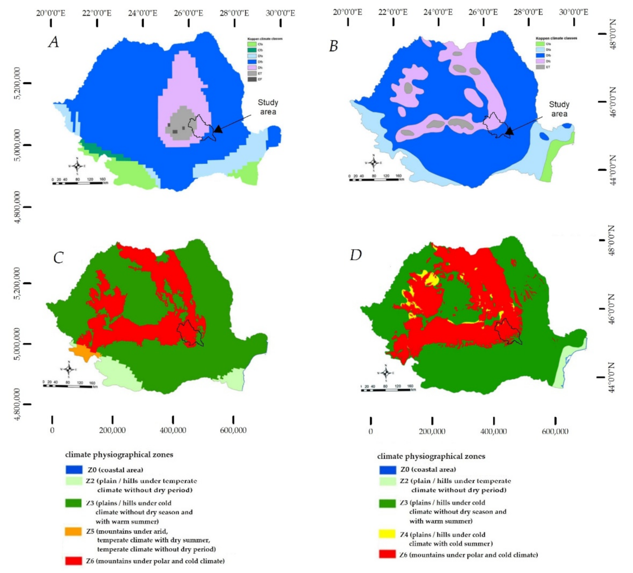
Considering that the influence of predisposing factors such as lithology, slope and land use on slope stability varies according to climatic conditions [17] made a climate-physiographical zonation map of Romania (Figure A1). The combination of Köppen’s climatic classification (according to the National Meteorological Administration (NMA), 2008) with that of the mountainous zones resulted in a climate-physiographical classification (Figure A1D). According to the latter, our study area is largely located in zone Z6-mountains under cold climate and, secondarily, towards the SE, in zone Z3-lowlands and hills under cold climate without a dry season and with a warm summer. Two small areas in the NW fall into the Z4 class of lowlands and hills under cold climate with a cold summer.
Climatic variables have a permanent and lasting effect on the behaviour of rock materials. Diurnal, monthly and seasonal variations in the air and soil temperatures, duration and intensity of precipitation, and quantitative variations in precipitation coupled with thermal variations are involved in the initiation of geomorphological processes [37].

2.3. Landslide Processes

The Curvature Subcarpathians are characterized by a large number and variety of landslides (shallow and medium-seated earth and debris slides and flows). They often associate with erosional processes, forming large complexes. In the Curvature Carpathians, common processes are high-magnitude deep-seated rock slides, compound and complex landslides, generally being old processes, considered periglacial or immediately postglacial, and showing periodic reactivations [43].
Several studies on landslide susceptibility have targeted the region at the Curvature of the Carpathians [44,45,46,47,48]. Based on semi-quantitative or quantitative assessments, they have shown that larger areas classified as highly and very highly susceptible to shallow landslides characterize the Subcarpathian hilly unit, whereas in the mountainous sector, these classes are much more restricted and appear mainly along the rivers. As for deep-seated landslides, the high and very high susceptibility classes are much more developed in the Carpathians. This situation conclusively reflects the typology of landslides in terms of magnitude [46]. Several landslide risk scenarios have been elaborated according to different factors: landslide-inducing precipitation under present and future climate conditions and earthquakes, such as the one of 4 March 1977 or one having a 100-year return period [49].

3. Inputs and Methods

3.1. Data

One of the most important steps in establishing the susceptibility map is to carry out an inventory of landslides in the study area. This not only allows estimating the importance of the phenomenon in the study area but also to elaborate an updated landslide database. Thus, the inventory allows the preparation and evaluation of landslide density maps for each factor and subsequently to calculate the susceptibility index.
To differentiate between the effects of different parameters on the initiation of mass movements and their effects on the spreading of the material after failure, the landslide area is subdivided into two zones, namely, the initiation (source) zone and the accumulation (indicated as runout) zone [23,50], so as to be able to obtain differentiated results.
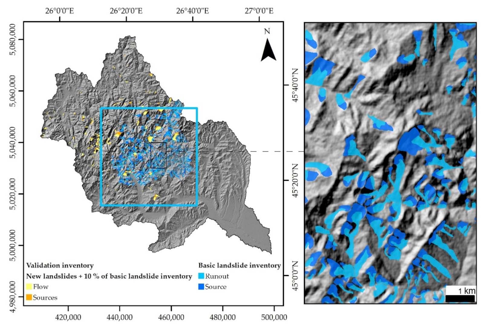
We used and completed the databases of Zumpano et al. [45] and Damen et al. [46]. The updating was based on the photo-interpretation of morphological landforms visible on high resolution satellite images (dating from 2009 to 2018) available on the Google Earth platform by digitising polygons of recent landslides still observable at a scale of 1:14,000. Subsequently, the landslide inventory was subdivided it into two parts (Figure 3), each containing the two landslide areas, source and runout. One data subset, composed of 1982 landslides, with 1029 source zones and 953 runout zones, was introduced in the calculation of the density map, while the other database, composed of 409 landslides with 206 source zones and 203 runout zones, was used for validation.
Sixteen parameters, predisposing, aggravating and triggering, were collected, processed and adapted to prepare them for the desired calculation process. While these data come from various sources at different scales (1/200,000, 1/5000, 1/14,000), we are aware that small-scale data may influence the model performance, but larger scale data were not always made available for the studied area. The following parameters were used: slope, geology, roughness, distance to the hydraulic network, topographic energy index (TPI), wetness, curvature, profile curvature, plane curvature, flow accumulation, internal friction angle (φ), cohesion (C), rock density (γ), distance to faults, distance to earthquakes and normalized difference vegetation index (NDVI).
To evaluate the dependency between these different explanatory variables, we calculated the correlation matrices for the source and runout (accumulation) areas, using the ‘Band Collection Statistics’ tool of the ArcMap platform (10.8.1). The tables in the appendix show the correlation matrices of the 16 parameters used (Table A2 and Table A3). Due to collinearity reasons, in the case of source areas, we eliminated the factors slope, curvature and the friction angle (φ). In the case of runout zones, we removed slope, curvature, cohesion and friction angle. This leaves 13 parameters for the source and 12 parameters for the runout susceptibility analyses.

3.2. Methods

3.2.1. Statistical Susceptibility Map

To establish the susceptibility maps, we applied the approach of the landslide factor analysis according to Vanacker et al. [23,24] but by including more diverse landslide factors. On the ArcMap platform, we transformed the shapefiles (polygon) of the landslide inventory into raster files (15 m grid). Thus, the landslide pixels inform about the presence of the two landslide components that were mapped: One raster map resulted for the source parts and a second raster map for the runout parts. These two specific landslide raster maps were then used to extract information from the other raster layers featuring morphological, geological, climatic and seismotectonic factors. Finally, we obtained a database of pixels subject to landslides. This allowed us to perform statistical analyses of the factors [24,51].
To calculate the density of landslide source or runout zones in a given class of a parameter (factor) within the catchment, we used the following formula [24,51]:
d i = N L P C N L P T × N P T N P C
where d i is the normalized landslide density in each class i , N L P C is the number of pixels affected by landslides in each class of the environmental factor, N L P T is the total number of pixels affected by landslides within the environmental factor map, N P T is the total number of pixels within the environmental factor map and N P C is the number of pixels in each class of the environmental factor map.
The results of this equation are presented in Table A1 for each environmental factor used. The susceptibility maps for the prediction of source and runout (accumulation) zones were obtained by calculating the geometric mean of the factors used according to the following formula [24]:
  S c = i = 1 n S c i n
where S c is the susceptibility, S c i the density of factors i and n the number of parameters.

3.2.2. Newmark’s Method

The Newmark method [52] is based on a simple model of the sliding of a block on an inclined plane. It aims to calculate the sliding distance, the ND, and is based on a double integration scheme of a time history of acceleration. For this purpose, only values above a certain value, i.e., the critical acceleration and the threshold acceleration necessary to initiate sliding, are taken into account [24]. Several simplified formulae have been proposed that relate the ND to the Arias intensity and the critical acceleration. The formula of Miles and Ho [53] is as follows:
log D = 1.46 · log I a 6.642 · a c + 1.546
where D is the displacement (cm), I a the Arias intensity (m/s) and a c the critical acceleration (m/s2).
The critical acceleration is given by the following formula [53,54]:
a c = F S 1 · g · sin α
where g is the gravitation (m/s2), α is the slope (°) and F S is the safety factor calculated according to the formula using the simplified Janbu’s method (original: in [55]):
F S = C γ · t · sin α + t a n   φ tan α m · γ w · tan φ γ · tan α
where C is the cohesion (MPa), φ is the angle of internal friction (°), t is the total thickness of the layer (m), m is the thickness of the saturated layer, γ w is the unit weight of the material (kg/m3) and γ is the unit weight of water (kg/m3).

3.2.3. Arias’ Intensity

The effect of earthquakes on the occurrence of mass movements is not negligible. This effect is introduced by the energy that propagates in the ground during earthquakes inducing complex periodic displacements that can unbalance the slopes. This displacement is measured by Arias [55], who gives the degree of ground shaking. This concept has been applied to the assessment of earthquake-induced landslide risk [53,54].
The seismic correlation of earthquake-induced slip with this intensity measure was first performed by Keefer and Wilson [56,57,58] developed a new generic formula that gives the I a and the Cumulative Absolute Velocity (CAV):
ln Y p r e d = c 0 + c 1   M w 5 + ( c 2 + c 3 M w ) ln ( R r u p 2 + H 2 ) 0.5 + c 4 F I n S l a b + c 5 ln V S 30 760 + e 1
where F I n S l a b is a dummy variable taking the value 1 for events occurring on the slab and 0 otherwise, M w is the magnitude, R is the distance, H is the depth of the hypocentre and V S 30 is the shear velocity (of S-waves) over a depth of 30 m. The coefficients are given by the author in Table 2.
The earthquakes with a magnitude greater than 7.0 that have struck the region around the studied catchment area since the year 984 (a period of 1036 years) are presented in Figure 4 (from [38]). Inside the catchment area, only earthquakes of magnitude M w = 7.1 have occurred, while in the NE of the catchment one earthquake of magnitude M w = 7.9 (maximum magnitude recorded over a period of 1036 years, in 1802) has also been recorded.
The calculations were performed for different magnitudes, i.e., M w = 7.1 and M w = 8 (supported by the M w = 7.9 event in 1802), and depths of the hypocenter D (D = 100, D = 150 and D = 200 km) and for different saturation rates ‘m’ (i.e., m = 0, m = 0.5 and m = 1). A total of 18 ND maps were produced (Table 3).

3.2.4. Evaluation of Model Results

To evaluate both the fitting and the prediction performances of the obtained susceptibility models, we used the ROC (receiver operating characteristic) curve, which measures the performance of a binary classifier that classifies items into two distinct groups based on several factors. In our case, the two classes are represented by the values 1—equivalent to true, i.e., landslide presence pixels, and the value 0—equivalent to false, i.e., landslide absence pixels.
The ROC curve provides both a graphical view and a relevant measure of the performance of a classifier [59,60]. Although several evaluation methods are available in the literature, the ROC curve is widely used to evaluate the outcome of landslide susceptibility maps [60,61,62]. The skill of the model and its discrimination ability are measured by the height of the curve above the diagonal line as well as by its steepness.
As is recommended [63], in addition to testing the statistical performance of the models, in a second phase, the geomorphological meaning and reliability were analysed in relation to the regional characteristics.

4. Results

4.1. Susceptibility Zonation Maps

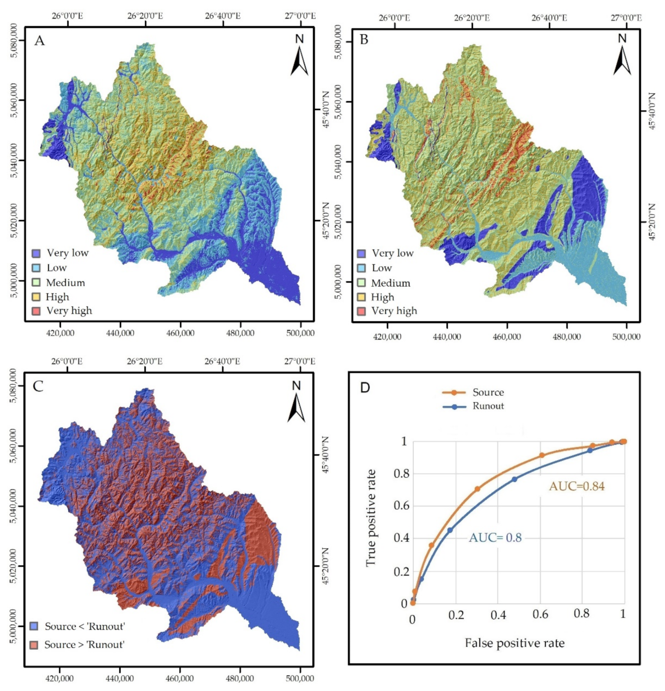
Two landslide susceptibility zonation maps were obtained: one for the source zones (source) and another for the runout zones of landslide material (runout). The susceptibility scale was classified into five equal-interval levels: very low [0–0.2], low [0.2–0.4], medium [0.4–0.6], high [0.6–0.8] and very high [0.8–1] (Figure 5A,B).
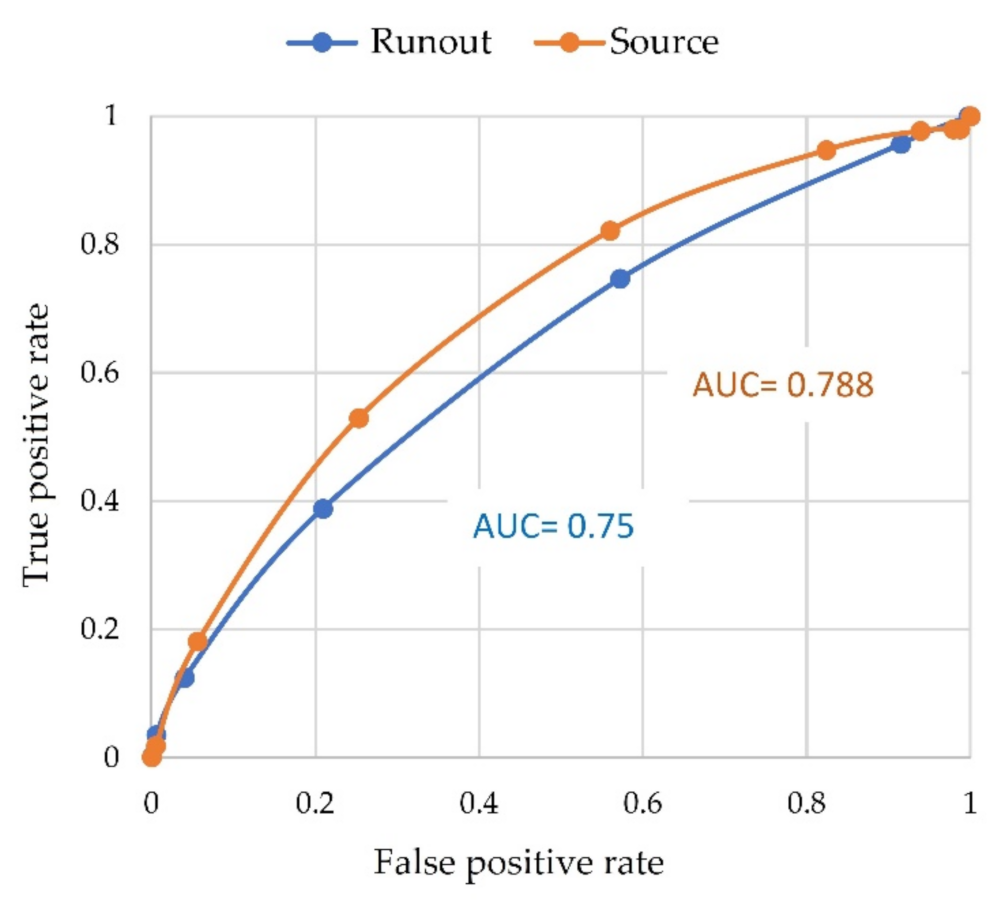
The evaluation of the fitting performance of susceptibility zones was conducted by calculating the ROC curves related to the calibration landslide dataset, while the prediction performance was tested by calculating the ROC curves in relation to the validation landslide dataset. The evaluation of the density map for the initiation zones (source) shows a ROC curve (Figure 5D) with an associated AUC of 0.84. The evaluation of the density map for the runout areas shows an upwardly convex ROC curve (Figure 5D) deviating from the straight line (45°), with an area under the curve (AUC) of 0.8. Both AUC values are greater than 0.7, which is, in practice, the value that justifies the validity of a classifier [64]. The ROC curves plotted in relation to the validation inventory (Figure A2) show AUC values of 0.79 and 0.75 for the source and the runout maps, respectively (values above the threshold for model validation [64]). These results show that the model has a valid and acceptable discrimination power. Indeed, the accuracy of the spatial distribution of susceptibility related to the source zones is higher than that related to the runout zones. This difference can be explained by the uncertainty in digitizing the boundaries of the runout zones, as they are less evident on the satellite images than in the case of source zones, which are clearly visible through the escarpments. This uncertainty could introduce non-runout pixels into the runout zones database and subsequently significantly influence the result.
The map of landslide source susceptibility (based on the landslide source zones; Figure 5A) shows a strong influence of the geological formations. High and very high susceptibility values are rendered for large areas in the Carpathian sector corresponding to the folded and faulted external (Paleogene) flysch units, in particular to the shale-sandstone flysch deposits and secondarily to the sandstone flysch. The southern border of this high-susceptibility area follows the limit between the mountains and the Subcarpathian hills. Such a distribution correlates with a predominance of large dormant landslides (deep-seated rock and debris slides and compound or complex landslides) featuring sectors of recent reactivations, partially located in the scarp areas. They are considered to be strongly connected to structural and tectonic characteristics, e.g., conditioned by faults which act as structural weaknesses during earthquakes [30]. The susceptibility values tend to decrease towards the north and northwest, where the intramontainous depression of Intorsura Buzăului lies. The inner Subcarpathian hills, underlain by intensely folded and faulted structures of Miocene molasse deposits, feature moderate landslide initiation susceptibility, although this unit is known to have an extremely large concentration of landslides ranging from slides to earth and debris flows. This situation could rather reflect the distribution of one certain landslide typology in terms of magnitude [46], namely, deep-seated movements, which register a much lower prevalence here than in the mountainous sector, pointing to a larger share held by deep-seated movements as opposed to shallow and medium-seated ones in the calibration landslide source dataset. Low and very low susceptibility areas are yielded for the south and southeast, in correspondence to the Pliocene-Quaternary strip of the outer Subcarpathian, as well as to the large floodplain and lowland areas. The Pliocene-Quaternary homocline relief, built on thick deposits with a high content of sands and gravels, features an interaction of landslides with erosional processes, the latter of which become slightly more predominant towards the exterior.
The susceptibility to landslide spreading (based on the landslide runout zones; Figure 5B) is highest in the median part of the basin and is elongated on a NE–SW direction parallel to the geological structures, located on the shale-sandstone flysch. High values also correspond to other mountain areas, where the lower slopes sectors are especially covered by thick landslide deposits, periodically affected by reactivation due to river deepening or forest cuttings. They are also encountered within the Miocene molasse deposits carved on less cohesive clays, marls or loose sandstones with clayey–marly intercalations, commonly subject to earth flows. Low and very low susceptibilities to landslide runout are registered along the outer Subcarpathian strip, made of Pliocene-Quaternary deposits mainly represented by sands and gravels, as well as in the lowlands.
The difference between the two susceptibility maps (Figure 5C) shows that the susceptibility to landslide accumulation is higher, i.e., indicative for a prevalence of flow-type of processes, in the inner Subcarpathian hills, where earth and debris flows are abundant. In addition, mountainous areas built of softer rocks (shale flysch, shale-sandstone flysch) are more susceptible to flows (where, indeed, typically mudflows, debris flows, compound and complex landsides are found). The central higher parts of the mountains, made-up of sandstone flysch, are clearly marked by higher source susceptibility values—which is consistent with the development of more massive rock slides featuring large scarp areas. The higher source susceptibility in the upper slope sectors, with massive landslides originating preferentially from the mountain crests, hints at the influence of seismic triggering of slope failures near the mountain tops that are exposed to stronger earthquake shaking.

4.2. Newmark Displacement Maps

According to the ROMPLUS catalogue [38], the hypocenter depths of 7.1 magnitude ( M w ) earthquakes vary between 100 and 150 km, although most are 150 km deep, as is the case of the M w = 7.9 earthquake, the single biggest magnitude earthquake in the region. To investigate different possible scenarios of these extreme cases, we calculated several models considering the following assumptions: For the whole basin, the thickness ( t ) of the layer subject to sliding was set to t = 10 m; the saturation rate m = 0 stands for totally dry conditions, m = 0.5 for half saturated conditions (half of the sliding layer, i.e., 5 m, is saturated) and m = 1 for 100% saturation (fully saturated over the 10 m sliding layer thickness). For the scenario calculations we also considered two magnitudes, namely, M w = 7.1 and M w = 8 .
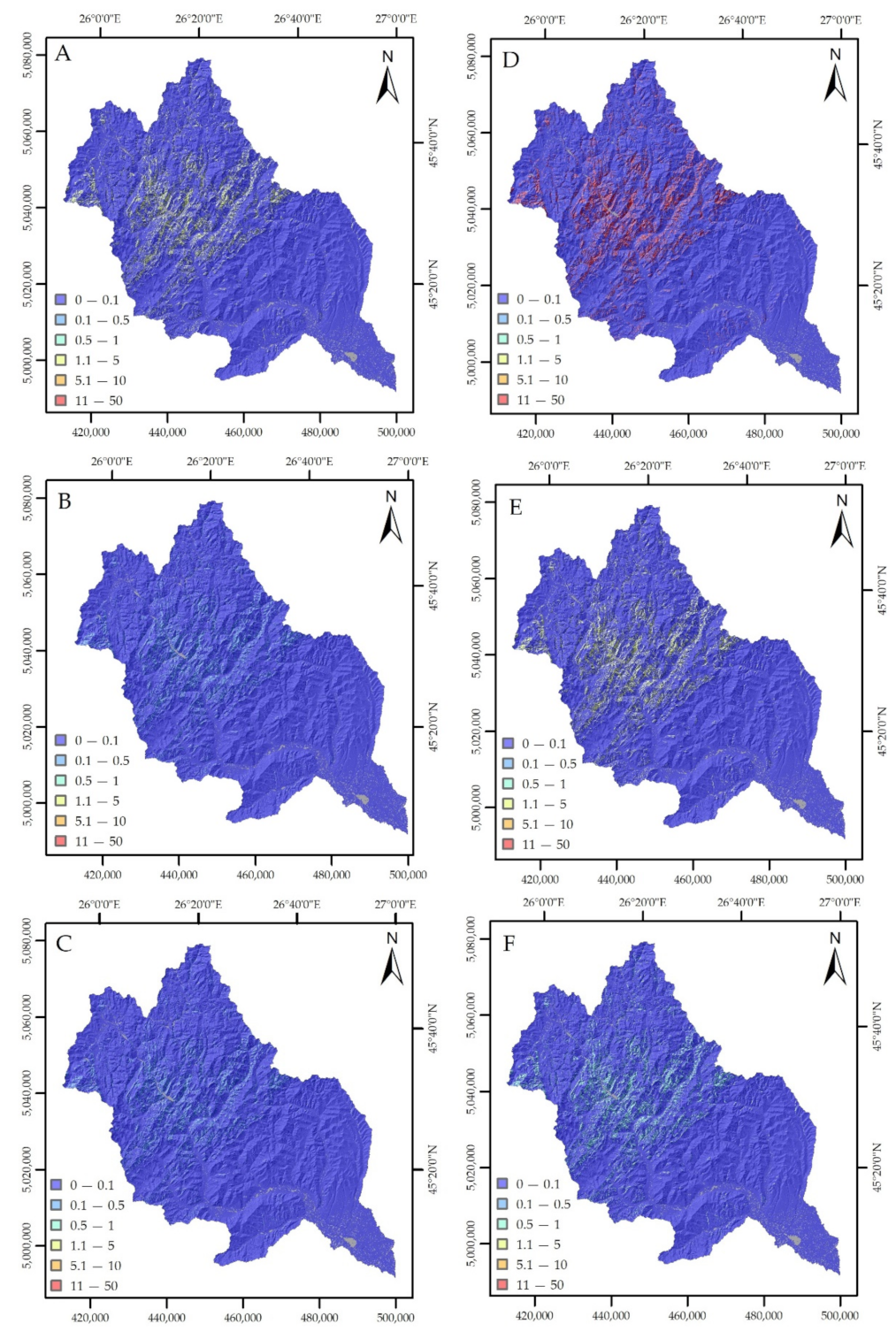
Eighteen maps of ND as a function of the saturation rate ( m ), magnitude and depth of the hypocentre were produced (Table 3). These 18 maps (Figure A3 and Figure 6) show that the most important displacements are related to the 100% saturation (m = 1, Figure 6). The map with the largest ND is the one considering a magnitude M w of 8 and a depth of 100 km with a maximum displacement of 50 cm (Figure 6B), while the one with the smallest ND is the map assuming a magnitude M w of 7.1 and a depth of 200 km (Figure A3C).
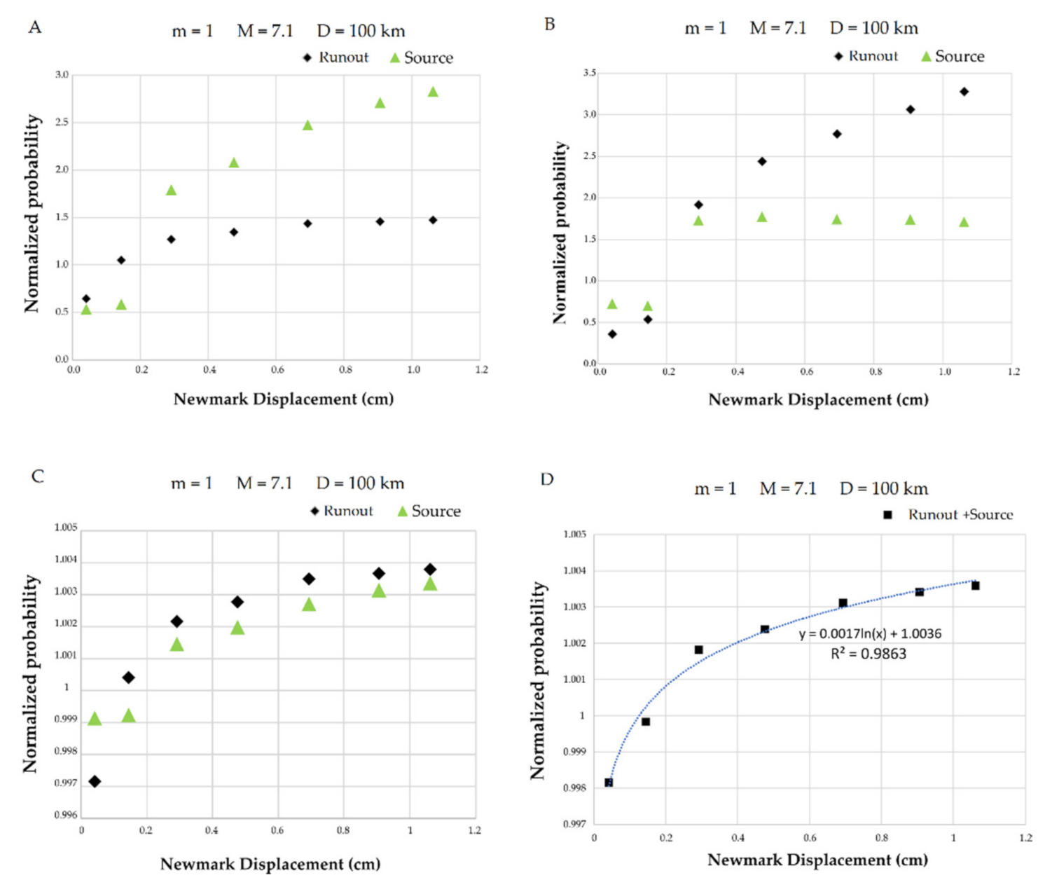
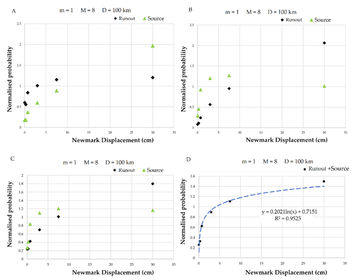
We consider as interesting maps the extreme case of magnitude M w = 8 and depth 100 km (even if, in the catalogue, earthquakes of this order have depths of 150 km) and that of magnitude M w = 7.1 at a 100 km depth, often produced in the basin. To validate these two maps, we performed a statistical analysis by calculating the normalized probability for the runout and source landslide zones separately and then for the two grouped together. This analysis was conducted on the landslide inventory used for validation and also on the landslide inventory used for the calibration of the susceptibility maps (Figure 7 and Figure 8).
The comparison of the 2 maps (Figure 6A,D) shows that the ND in the M w = 8 map is 10 times greater than that in the M w = 7.1 map. The maximum values are located in the centre of the basin within the Carpathian Curvature, generally located in the concave surfaces of the mountainsides. These can focus the seismic energy and amplify the amplitude (site effect), thus enhancing the potential for mass movement triggering as compared to other locations with convex topographic surfaces.
For the magnitude M w = 7.1 map model (Figure 6A), the normalised probability of landslides (of any type) is directly related to the ND. It increases proportionally with the ND (Figure 7A,B). The runout zones behave differently from the source ones, as the runout zones show a logarithmic curve, with a steep slope at the beginning followed by a very low slope plateau. The source zones show a stable plateau at the start and then a logarithmic behaviour. For the calibration landslide dataset, the pattern is the same as for the validation landslides, except that, this time, the probability of the runout zones is higher than that of the source zones. The normalised probability of the two grouped inventories (Figure 7C) illustrates a similar trend between sources and runouts from the 0.1 cm displacement. The general trend for the combined runout and source zones of both databases shows a rapid increase in the normalised probability between displacements 0 cm to 0.2 cm and then another stage with a small increase according to the following logarithmic law (Figure 7D):
Y = 0.00017   l n x + 1.0036
The M w = 8 map (Figure 6D) also has curves similar to the M w = 7.1 map, logarithmically increasing the normalised probability with ND (Figure 8). For all landslides in both databases, the normalised probability varies according to the following logarithmic law (Figure 8D):
Y = 0.2021   l n x + 0.7151
The difference between the normalised probability of the models for the simulated M w = 7.1 and M w = 8 (represented in Figure 7 and Figure 8, respectively) is equivalent to the maximum displacement values of 1.2 cm for the M w = 7.1 scenario and of 30 cm for the M w = 8 scenario. Additionally, according to Equations (7) and (8) for the same displacement (x), we have the relationship between Y 7.1 (normalised probability of the M w = 7.1 model) and the Y 8 (normalised probability of M w = 8 model):
Y 8 = 1189   Y 7.1 + 1194
This shows that for the same displacement value, the normalised probability of the magnitude M w = 8 model is greater than the normalised probability of the magnitude M w = 7.1 . So, the difference of 0.9 magnitude units causes this large influence on the normalised probability.

5. Discussion and Conclusions

Landslide susceptibility zonation maps are generally calculated based on several environmental factors that authors consider to be the most important according to the climate-morphostructural and geodynamic contexts and the data available at the time of the study. In the literature, there are no standard environmental factors (norms) that must imperatively be used to establish a susceptibility zonation, especially as the calculation approaches are diverse. It is a common practice to search for correlations among these factors in order to reduce their number and eliminate redundant information. For a given model and apart from the mathematical means and techniques of validation which can ‘show’ satisfactory results (acceptable errors), ‘expert’ validation in the field is indispensable for the adjustment and correct interpretation of an obtained model.
The comparison of susceptibility zonation maps and ND maps can only be achieved by understanding the meaning and/or physical concept of the magnitude given by each map. The ND maps indicate the maximum displacement of the ground during an earthquake: the larger the displacement, the higher the susceptibility for landslides. However, it is difficult to establish a threshold (minimum value) of ND that can trigger a landslide if it is associated with other factors. Even if we have data on landslides caused by some earthquakes, we do not really know if the displacement generated by these earthquakes is the minimum that was needed to cause the trigging or if there was an additional contribution which was responsible for the observed failures. Even if the ND is a physical quantity, it is based on a statistical calculation, so the interpretation of displacements has a relative aspect. Moreover, even if we have the maximum displacement in several places, those places do not contain any landslide occurrences, which indicates that there are other factors that come into play in addition to the ND. In the case of susceptibility zonation maps, these represent the total influence of environmental factors according to their spatial distributions. This concept, which is different from that of ND maps, allows a high number of factors that are deemed useful to be considered and introduced into the model (in this study we used 16 factors). The comparison of the two types of maps helps combine the advantages of a statistical method with those of a process-based one.
The comparison between the susceptibility zonation maps and the ND maps is carried out firstly by spatial correlation between the four maps (Table 4; Table 5). Secondly, the comparison is made visually by looking at the patterns of the maps according to the geographical areas (Figure 9). The two ND maps (magnitudes M w = 7.1 and M w = 8 ) are very well correlated with each other, which is logical as the only difference in the calculation of the two maps is the energy of the earthquake. Yet, there are also differences: First, it can be noticed that the landslide source zonation can be better correlated with the ND maps ( M w = 7.1 and M w = 8 ) than the accumulation zonation. The five locations that show a marked difference between the maps of runout susceptibility and ND generated by magnitude M w = 7.1 (Figure 9B,C) are Dălghiu, NW of Barcani, SE of Pătârlagele, Murgeşti and S of Pârscov. The source zonation shows the lowest susceptibility in these areas while the ND is large, especially at Dălghiu (1.8 to 2.5 cm) (Figure 9A,C). The highest susceptibilities that correspond to the largest ND are distributed along a SW–NE direction, passing through Nehoiu, Gura Teghii and Lopătari towards Secuiu. Further analysis using unmanned aerial vehicles should focus on these locations in other to better understand the local environmental conditions with up-to-date very-high-resolution imagery and elevation models [65]. The Buzău floodplain in the plain unit shows low values of both ND and susceptibility. To summarize, the zonation of landslide initiation susceptibility (Figure 9A) shows a distribution more similar to the ND (Figure 9C), with the difference being especially marked in the mountains (Dălghiu, Intorsura Buzăului and west of Barcani). The direction of this agreement between the two maps correlates well to the main structures. This is consistent with the fact that the landslide source prediction more closely reflects the spatial distribution patterns of deep-seated landslides, many of which show a high probability of being linked to a seismic cause (e.g., large scarps close to the ridge-tops, vicinity to fault lines, accumulation sectors with no apparent interaction with the river network) [43].
One uncertainty affecting the output landslide source and accumulation susceptibility patterns stems from the spatial incompleteness and heterogeneity of the landslide inventory used in the analysis. This dataset is mostly constrained to the area mapped by Zumpano et al. [45] and Damen et al. [46], hence it does not cover the entire study area. Completion of the landslide data outside this area was rather difficult. Especially in the northern sector, landslide detection was rendered almost impossible due to the increased surface covered by forests. Since the ratio of areas corresponding to factor classes within the landslide sample area cannot be the same as for the whole study area, calculating landslide densities in relation to entire class areas is suspected to produce biased outputs. This situation applies, for instance, to the lithological class ‘sands with marls and clays, locally gravels’ present especially in the SE of the study area, for which almost no information on landslides could be extracted from the mapped sample. Nevertheless, statistically, this translated into a ‘zero density’, thus cancelling the predisposition for landslide runout susceptibility throughout the study area where the respective lithology appears. Future improvements of the predictions are expected if either using a landslide database with a better coverage across the study area or enhancing the representativeness of the landslide sample, restricting the susceptibility computations to the sample area, and finally extrapolating the results to the entire study area.
Additionally, considering the differences in the distribution of shallow versus deep-seated landslides, typologically differentiated landslide initiation and runout susceptibility assessments are envisaged for a future work. This could have an impact when comparing the deep-seated landslide source susceptibility map with ND maps, since it was shown that numerous such processes have a morphology showing a potential involvement of the seismic factor [43].
In order to improve the ND map, since the parameter ‘m’ (water saturation) has a significant influence on the result, different values of ‘m’ should be assigned to the different lithologies, considering that permeability and water retention vary according to the rock type, which controls the saturation rate. Adding a general ‘m’ value to all pixels of the study area does not allow to ‘introduce’ the differentiated effect of water specific for the different lithological formations. This parameter also varies according to the season, so future work will aim to establish separate maps for the wet period (m = 1, typically for the months of March–June and October–December) and for the dry period (m = 0–0.5, corresponding to June–September, January–February), while also taking into account the variation of ‘m’ with geology.
In addition, the parameter ‘t’ (thickness of the layer, fixed at 10 m in this study), used in the calculation of the safety coefficient (above), is a parameter that can highly vary over the mapped area. However, defining the relative thickness of landslides for different slope conditions, geological conditions, proximities to rivers and vegetation covers is difficult. Possibly, some remote- or close-sensing-based analyses could help establish some statistical links between landslide thicknesses and local factors influencing slope instability.
Moreover, one could also consider that instead of purely comparing the single ND map with the statistical landslide susceptibility zonation maps, it could be interesting to introduce the ND map as one of the environmental factors used for the calculation of the susceptibility zonation map. This could be achieved in the frame of a more detailed future study.
Finally, it might be helpful to introduce the effect of differential weathering caused by climatic conditions as an environmental factor in the landslide susceptibility mapping procedure or via the ‘t’ factor in the ND map calculation. Indeed, the ageing of the rock implies its alteration on the surface, which controls its mechanical weakening and consequently its susceptibility to ground movements. The same lithology does not necessarily have the same physical properties—which evolve over time and change with the slope’s exposure (orientation with respect to wind and sun radiation effects) due to variable fracturing, the leaching rate by meteoric water, the presence of groundwater, etc. However, collecting related information over such wide areas represents a major challenge.

Author Contributions

Conceptualization, H.H. and R.S.; methodology, H.H.; software, H.H.; validation, R.S., M.J. and H.-B.H.; formal analysis, H.H.; investigation, H.H.; resources, H.-B.H.; data curation, H.H.; writing—original draft preparation, H.H.; writing—review and editing, H.H., R.S., M.J. and H.-B.H.; visualization, R.S.; supervision, H.-B.H.; project administration, H.-B.H.; funding acquisition, H.-B.H. All authors have read and agreed to the published version of the manuscript.

Funding

H. Harmouzi received a scholarship funded by IN WBI Excellence (Belgian funding scheme).

Data Availability Statement

Unless specified differently, data and imagery used for this publication are freely available from the following providers or software: ArcGIS/Credit: Esri (version 10.5.1); Google Earth Pro/Credit: Google 2020 (version 7.3.3); SRTM 1 Arc-Second Global/Credit: USGS. Data available at https://earthexplorer.usgs.gov/ (accessed on 19 February 2021); EM-DAT. Natural disasters 2019: Now is the time to not give up. The CRED/USAD. International disaster database. Université’ Catholique de Louvain, Brussels, 2020. www.em-dat.net (accessed on 30 June 2021); EEA. Mapping the impacts of natural hazards and technological accidents in Europe: an overview of the last decade. European Environmental Agency Technical report 13. Office for Official Publications of the European Union, Luxembourg, 2010 (accessed on 30 June 2021); NIEP. ROMPLUS Catalogue data available online at http://www.infp.ro/index.php?i=romplus (accessed on 9 July 2021).

Acknowledgments

We are grateful for the support of Mihai Micu (Institute of Geography, Romanian Academy) for providing landslide inventory data for the study region, and permitting to use it for the analysis. We are also thankful to Lucian Badea, Adrian Grozavu (Faculty of Geography and Geology, Alexandru Ioan Cuza University of Iași, Romania), Cristian Patriche (Geography Group, Romanian Academy, Iași Branch, Romania) and Florina Grecu for granting us the permission to reproduce their maps and figures used in characterizing the study region. We would like to acknowledge the free earthquake data provided by the National Institute for Earth Physics (NIEP) through the ROMPLUS Catalogue. The authors express their thanks to Philippe Cerfontaine for the computer advice and for the data conversion. We also thank Brigitte Ernst from the Liège University administration who helped during all the stages of the main author’s internship. The study also partially benefitted from the work done in the frame of the Romanian Academy research project “Geographical studies within the Natural Hazards Research Centre of Pătârlagele, Buzău County”, coordinated by the Institute of Geography.

Conflicts of Interest

The authors declare no conflict of interest.

Appendix A

Figure A1. Location of the study area on the maps of: Köppen climate classification according to Peel et al. [33] (A) and Grozavu et al. [17] (B); climate-physiographical zones according to Wilde et al. [10] (C) and Grozavu et al. [17] (D). From [17]. Reproduced with permission from Grozavu, A., Patriche, C., Geomatics, Natural Hazards and Risk; published by Taylor & Francis Group, 2021.
Geosciences 11 00495 g0a1
Figure A2. Susceptibility ROC curves constructed using the validation database.
Geosciences 11 00495 g0a2
Figure A3. ND maps (cm) for saturation rate m = 0.5 , magnitude M w = 7.1 (depths D = 100   km (A), D = 150   km (B), D = 200   km (C)); magnitude M w = 8 (depths D = 100   km (D), D = 150   km (E), D = 200   km (F)).
Geosciences 11 00495 g0a3
Table A1. Landslide densities computed for the classes of the different factors. (Bolded and underlined values indicate maximum densities).
ClassesSlope (Degrees)dRuggednessdDistance to the Hydrographic NetworkdDominant Formation of the Lithological Class dWetnessdTopographic Position Index (TPI)dCurvaturedProfile Curvatured
Source0–9.130.170–1.870.170–1660.33Alluvial dep0.100.87–2.462.03(−12.08)–(−1.55)1.23(−19.14)–(−1.92)1.21(−14.84)–(−1.23)1.57
9.13–17.700.821.87–3.80.84166–3491.04Sandstones1.292.46–4.371.64(−1.55)–(−0.95)1.43(−1.92)–(−1.19)1.41(−1.23)–(−0.75)1.55
17.70–26.261.813.8–5.741.87349–5331.69Shales/clays1.624.37–6.280.90(−0.95)–(0.36)1.28(−1.19)–(−0.46)1.28(−0.75)–(−0.27)1.30
26.26–34.833.045.74–7.693.01533–7162.05Sands0.026.28–8.180.29(−0.36) –0.230.80(−0.46) –0.270.81(−0.27)–0.190.83
34.83–66.463.357.69–26.733.37716–10671.91Salt0.008.18–10.090.130.23–0.821.120.27–1.001.110.19–0.671.12
10.09–14.590.070.82–1.421.421.00–1.741.410.67–14.211.22
1.42–20.111.481.74–27.891.46
Runout0–9.130.750–1.870.760–1661.50Alluvial dep0.410.87–2.460.34(−12.08)–(−1.55)0.85(−19.14)–(− 1.92)0.85(−14.84)–(−1.23)0.38
9.13–17.701.341.87–3.81.32166–3490.89Sandstones1.122.46–4.370.42(−1.55)–(−0.95)1.28(−1.92) – (−1.19)1.25(−1.23)–(−0.75)0.47
17.70–26.260.893.8–5.740.88349–5330.58Shales/clays1.994.37–6.281.25(−0.95)–(−0.36)1.50(−1.19) – (−0.46)1.48(−0.75)–(−0.27)0.73
26.26–34.830.655.74–7.690.65533–7160.32Sands0.006.28–8.181.57(−0.36)–0.231.02(−0.46)–0.271.03(−0.27) –0.191.01
34.83–66.460.497.69–26.730.51716–10670.30Salt0.008.18–10.091.510.23–0.820.740.27–1.000.750.19–0.671.27
10.09–14.590.970.82–1.420.461.00–1.740.470.67–14.211.10
1.42–20.110.371.74–27.890.38
ClassesPlane CurvaturedFlow AccumulationdAngle of Internal Friction (φ)dCohesion (C)dRock Density (ϒ)dDistance to the FaultsdDistance to the EpicentersdNormalized Difference Vegetation Index (NDVI)d
Source(−9.89)–(−1.05)1.470–20.54200.0400.001.90.060 –501.580–5512.030.39–0.640.60
(−1.05)–(−0.64)1.582–61.39252.800.050.1020.0050–1001.60551–11850.520.64–0.652.39
(−0.64)–(−0.23)1.366–121.52280.910.11.012.31.45100–5001.721194–18280.190.65–0.652.42
(−0.23)–0.170.7912–271.20320.010.20.00 500–10001.731819–44410.030.65–0.651.97
0.17–0.581.0427–1.7E+170.69351.0112.80 1000–320000.44 0.65–0.652.34
0.58–0.991.31 0.65–0.801.30
0.99–13.041.35
Runout(−9.89)–(−1.05)0.930–20.43200.0000.001.90.210–502.210–5512.020.39–0.640.70
(−1.05)–(−0.64)1.362–60.90253.410.050.4120.0050–1002.19551–11850.550.64–0.652.17
(−0.64)–(−0.23)1.486–121.23282.900.10.882.31.38100–5001.851194–18280.160.65–0.652.28
(−0.23)–0.170.9612–271.71320.130.20.00 500–10001.641819–44410.020.65–0.652.89
0.17–0.580.8027–1.7E+171.89350.8813.41 1000–32,0000.36 0.65–0.652.46
0.58–0.990.53 0.65–0.801.19
0.99–13.040.38
Table A2. Correlation matrix of parameters for landslide source susceptibility. (Values in bold indicate high correlations).
Physical ParametersNorm. Diff. Vegetation Index (NDVI)RuggednessDist. to the FaultsDist. to Earthquake EpicentresSlopeTopographic Position Index (TPI)Cohesion (C)CurvatureDist. to the Hydro. NetworkFlow AccumulationWetnessRock Density (γ)LithologyAngle of Internal Friction (Φ)Plan CurvatureProfile Curvature
Norm. Diff. Vegetation Index (NDVI)1.00.30.50.30.30.20.40.20.10.00.30.50.50.40.20.2
Ruggedness0.31.00.20.21.00.30.20.30.10.00.60.40.30.20.20.2
Dist. to the Faults0.50.21.00.20.20.20.40.20.00.00.20.50.50.40.20.2
Dist. to Earthquake Epicentres0.30.20.21.00.20.10.20.10.00.00.10.20.30.30.10.1
Slope0.31.00.20.21.00.30.20.30.10.00.60.40.30.20.20.2
Topographic Position Index (TPI)0.20.30.20.10.31.00.10.90.0-0.10.20.20.20.20.50.5
Cohesion (C)0.40.20.40.20.20.11.00.10.10.00.20.50.81.00.10.1
Curvature0.20.30.20.10.30.90.11.00.0−0.10.20.20.20.10.50.5
Dist. to the Hydr. Network0.10.10.00.00.10.00.10.01.00.00.30.10.10.10.00.0
Flow Accumulation0.00.00.00.00.0−0.10.0−0.10.01.00.10.00.00.0−0.1−0.1
Wetness0.30.60.20.10.60.20.20.20.30.11.00.30.20.20.10.1
Rock Density (γ)0.50.40.50.20.40.20.50.20.10.00.31.00.70.50.20.2
Lithology0.50.30.50.30.30.20.80.20.10.00.20.71.00.80.20.2
Angle of Internal Friction (Φ)0.40.20.40.30.20.21.00.10.10.00.20.50.81.00.20.2
Plan Curvature0.20.20.20.10.20.50.10.50.0−0.10.10.20.20.21.01.0
Profile Curvature0.20.20.20.10.20.50.10.50.0−0.10.10.20.20.21.01.0
Table A3. Correlation matrix of parameters for landslide runout susceptibility. (Values in bold indicate high correlations).
Physical ParametersNorm. diff. Vegetation Index (NDVI)RuggednessDist. to the FaultsDist. to Earthquake EpicentresSlopeTopographic Position Index (TPI)Cohesion (C)CurvatureDist. to the Hydro. NetworkFlow AccumulationWetnessRock Density (γ)LithologyAngle of Internal Friction (Φ)Plan CurvatureProfile Curvature
Norm. Diff. Vegetation iIndex (NDVI)1.00.10.30.10.10.0−0.20.20.00.0−0.20.40.20.20.00.0
Ruggedness0.11.00.20.00.00.0−0.10.20.00.0−0.10.20.20.20.00.0
Dist. to the Faults0.30.21.00.10.10.0−0.20.30.00.0−0.20.50.40.30.00.0
Dist. to Earthquake Epicentres0.10.00.11.00.90.00.00.10.0−0.1−0.30.10.10.10.00.0
Slope0.10.00.10.91.00.00.00.10.0−0.1−0.30.10.10.10.00.0
Topographic Position Index (TPI)0.00.00.00.00.01.00.30.01.00.1−0.50.00.00.00.60.7
Cohesion (C)−0.2−0.1−0.20.00.00.31.0−0.10.30.3−0.3−0.3−0.1−0.10.30.2
Curvature0.20.20.30.10.10.0−0.11.00.0−0.1−0.10.40.90.90.00.0
Dist. to the Hydr. Network0.00.00.00.00.01.00.30.01.00.1−0.50.00.00.00.60.7
Flow Accumulation0.00.00.0−0.1−0.10.10.3−0.10.11.0−0.4−0.1−0.10.00.00.1
Wetness−0.2−0.1−0.2−0.3−0.3−0.5−0.3−0.1−0.5−0.41.0−0.1−0.1−0.1−0.5−0.7
Rock Density (γ)0.40.20.50.10.10.0−0.30.40.0−0.1−0.11.00.60.30.0−0.1
Lithology0.20.20.40.10.10.0−0.10.90.0−0.1−0.10.61.00.80.00.0
Angle of Internal Friction (Φ)0.20.20.30.10.10.0−0.10.90.00.0−0.10.30.81.00.00.0
Plan Curvature0.00.00.00.00.00.60.30.00.60.0−0.50.00.00.01.00.3
Profile Curvature0.00.00.00.00.00.70.20.00.70.1−0.7−0.10.00.00.31.0

References

  1. European Environmental Agency. Mapping the Impacts of Natural Hazards and Technological Accidents in Europe—An Overview of the Last Decade; Publications Office of the European Union: Luxembourg, 2010; p. 144. [Google Scholar]
  2. Centre for Research on the Epidemiology of Disasters. Natural Disasters 2019: Now Is the Time to Not Give Up; CRED: Brussels, Belgium, 2020. [Google Scholar]
  3. Alexander, E.D. Vulnerability to Landslides. In Landslide Risk Assessment; Glade, T., Anderson, M., Crozier, M., Eds.; Wiley: Hoboken, NJ, USA, 2005; pp. 175–198. [Google Scholar]
  4. Nadim, F.; Kjekstad, O.; Peduzzi, P.; Herold, C.; Jaedicke, C. Global Landslide and Avalanche Hotspots. Landslides 2006, 3, 159–173. [Google Scholar] [CrossRef]
  5. Hong, Y.; Adler, R.; Huffman, G. Use of Satellite Remote Sensing Data in the Mapping of Global Landslide Susceptibility. Nat. Hazards 2007, 43, 245–256. [Google Scholar] [CrossRef] [Green Version]
  6. Kirschbaum, D.; Adler, R.; Hong, Y.; Lerner-Lam, A. Evaluation of a Preliminary Satellite-Based Landslide Hazard Algorithm Using Global Landslide Inventories. Nat. Hazards Earth Syst. Sci. 2009, 9, 673–686. [Google Scholar] [CrossRef] [Green Version]
  7. Dilley, M.; Chen, R.S.; Deichmann, U.; Lerner-Lam, A.; Arnold, M.; Agwe, J.; Buys, P.; Kjekstad, O.; Lyon, B.; Yetman, G. Natural Disaster Hotspots: A Global Risk Analysis; The World Bank: Washington, DC, USA, 2005. [Google Scholar] [CrossRef]
  8. Günther, A.; Eeckhaut, M.; Malet, J.-P.; Paola, R.; Hervás, J. Climate-Physiographically Differentiated Pan-European Landslide Susceptibility Assessment Using Spatial Multi-Criteria Evaluation and Transnational Landslide Information. Geomorphology 2014, 224, 69–85. [Google Scholar] [CrossRef]
  9. Jaedicke, C.; Eeckhaut, M.; Nadim, F.; Hervás, J.; Kalsnes, B.; Vangelsten, B.; Smith, J.; Tofani, V.; Ciurean, R.; Winter, M.; et al. Identification of Landslide Hazard and Risk ‘Hotspots’ in Europe. Bull. Eng. Geol. Environ. 2014, 73, 325–339. [Google Scholar] [CrossRef] [Green Version]
  10. Wilde, M.; Günther, A.; Reichenbach, P.; Malet, J.-P.; Hervás, J. Pan-European Landslide Susceptibility Mapping: ELSUS Version 2. J. Maps 2018, 14, 97–104. [Google Scholar] [CrossRef] [Green Version]
  11. Malet, J.-P.; Thiery, Y.; Hervás, J.; Günther, A.; Puissant, A.; Grandjean, G. Landslide Susceptility Mapping at 1:1 M Scale over France: Exploratory Results with a Heuristic Model. In Proceedings of the International Conference on Landslide Processes: From Geomorphologic Mapping to Dynamic Modelling; Malet, J.-P., Remaître, A., Boogard, T., Eds.; CERG Editions: Strasbourg, France, 2009; pp. 315–320. [Google Scholar]
  12. Okalp, K.; Akgün, H. National Level Landslide Susceptibility Assessment of Turkey Utilizing Public Domain Dataset. Environ. Earth Sci. 2016, 75, 847. [Google Scholar] [CrossRef]
  13. Peduzzi, P. Landslides and Vegetation Cover in the 2005 North Pakistan Earthquake: A GIS and Statistical Quantitative Approach. Nat. Hazards Earth Syst. Sci. 2010, 10, 623–640. [Google Scholar] [CrossRef]
  14. Abella, E.A.C.; Van Westen, C.J. Generation of a Landslide Risk Index Map for Cuba Using Spatial Multi-Criteria Evaluation. Landslides 2007, 4, 311–325. [Google Scholar] [CrossRef] [Green Version]
  15. Quesada-Román, A. Landslide Risk Index Map at the Municipal Scale for Costa Rica. Int. J. Disaster Risk Reduct. 2021, 56, 102144. [Google Scholar] [CrossRef]
  16. Bălteanu, D.; Micu, M.; Jurchescu, M.; Malet, J.-P.; Sima, M.; Kucsicsa, G.; Dumitrică, C.; Petrea, D.; Mărgărint, M.C.; Bilaşco, Ş.; et al. National-Scale Landslide Susceptibility Map of Romania in a European Methodological Framework. Geomorphology 2020, 371, 107432. [Google Scholar] [CrossRef]
  17. Grozavu, A.; Patriche, C. Mapping Landslide Susceptibility at National Scale by Spatial Multi-Criteria Evaluation. Geomat. Nat. Hazards Risk 2021, 12, 1127–1152. [Google Scholar] [CrossRef]
  18. Cepeda, J.M.; Høeg, K.; Nadim, F. Landslide-Triggering Rainfall Thresholds: A Conceptual Framework. Q. J. Eng. Geol. Hydrogeol. 2010, 43, 69–84. [Google Scholar] [CrossRef]
  19. Kumar, V.; Cauchie, L.; Mreyen, A.-S.; Micu, M.; Havenith, H.-B. Evaluating Landslide Response in Seismic and Rainfall Regime: A Case Study from the SE Carpathians, Romania. Nat. Hazards Earth Syst. Sci. Discuss. 2021, in press. [Google Scholar] [CrossRef]
  20. Quesada-Román, A.; Fallas López, B.; Hernandez-Espinoza, K.; Ballesteros-Canovas, J. Relationships between Earthquakes, Hurricanes, and Landslides in Costa Rica. Landslides 2019, 16, 1539–1550. [Google Scholar] [CrossRef]
  21. Carrara, A.; Cardinali, M.; Guzzetti, F.; Paola, R. GIS Technology in Mapping Landslide Hazard. In Geographical Information Systems in Assessing Natural Hazards; Carrara, A., Guzzetti, F., Eds.; Springer: Dordrecht, The Netherlands, 1995; Volume 5, pp. 135–176. [Google Scholar]
  22. Steger, S.; Kofler, C. Statistical Modeling of Landslides: Landslide Susceptibility and Beyond. In Spatial Modeling in GIS and R for Earth and Environmental Sciences; Pourghasemi, H.R., Gokceoglu, C., Eds.; Elsevier: Amsterdam, The Netherlands, 2019; pp. 519–546. ISBN 978-0-12-815226-3. [Google Scholar]
  23. Vanacker, V.; Vanderschaeghe, M.; Govers, G.; Willems, E.; Poesen, J.; Deckers, J.; De Bièvre, B. Linking Hydrological, Infinite Slope Stability and Land-Use Change Models through GIS for Assessing the Impact of Deforestation on Slope Stability in High Andean Watersheds. Geomorphology 2003, 52, 299–315. [Google Scholar] [CrossRef]
  24. Havenith, H.-B.; Strom, A.; Caceres, F.; Pirard, E. Analysis of Landslide Susceptibility in the Suusamyr Region, Tien Shan: Statistical and Geotechnical Approach. Lanslides 2006, 3, 39–50. [Google Scholar] [CrossRef]
  25. Dao, D.V.; Jaafari, A.; Bayat, M.; Mafi-Gholami, D.; Qi, C.; Moayedi, H.; Phong, T.V.; Ly, H.-B.; Le, T.-T.; Trinh, P.T.; et al. A Spatially Explicit Deep Learning Neural Network Model for the Prediction of Landslide Susceptibility. CATENA 2020, 188, 104451. [Google Scholar] [CrossRef]
  26. Merghadi, A.; Yunus, A.P.; Dou, J.; Whiteley, J.; ThaiPham, B.; Bui, D.T.; Avtar, R.; Abderrahmane, B. Machine Learning Methods for Landslide Susceptibility Studies: A Comparative Overview of Algorithm Performance. Earth-Sci. Rev. 2020, 207, 103225. [Google Scholar] [CrossRef]
  27. Hakimov, F.; Domej, G.; Ischuk, A.; Reicherter, K.; Cauchie, L.; Havenith, H.-B. Site Amplification Analysis of Dushanbe City Area, Tajikistan to Support Seismic Microzonation. Geosciences 2021, 11, 154. [Google Scholar] [CrossRef]
  28. Ozturk, U.; Pittore, M.; Behling, R.; Roessner, S.; Andreani, L.; Korup, O. How Robust Are Landslide Susceptibility Estimates? Landslides 2021, 18, 681–695. [Google Scholar] [CrossRef]
  29. Schlögel, R.; Marchesini, I.; Alvioli, M.; Paola, R.; Rossi, M.; Malet, J.-P. Optimizing Landslide Susceptibility Zonation: Effects of DEM Spatial Resolution and Slope Unit Delineation on Logistic Regression Models. Geomorphology 2017, 301, 10–20. [Google Scholar] [CrossRef]
  30. Micu, M. Landslide Types and Spatial Pattern in the Subcarpathian Area. In Landform Dynamics and Evolution in Romania; Springer Geography; Rădoane, M., Vespremeanu-Stroe, A., Eds.; Springer: Cham, Switzerland, 2017; pp. 305–325. ISBN 978-3-319-32587-3. [Google Scholar]
  31. Eeckhaut, M.; Hervás, J.; Jaedicke, C.; Malet, J.-P.; Montanarella, L.; Nadim, F. Statistical Modelling of Europe-Wide Landslide Susceptibility Using Limited Landslide Inventory Data. Landslides 2012, 9, 357–369. [Google Scholar] [CrossRef]
  32. Micu, M.; Jurchescu, M.; Șandric, I.; Margarint, M.C.; Chițu, Z.; Micu, D.; Ciurean, R.; Ilinca, V.; Vasile, M. Mass Movements. In Landform Dynamics and Evolution in Romania; Rădoane, M., Vespremeanu-Stroe, A., Eds.; Springer International Publishing: Cham, Switzerland, 2017; pp. 765–820. ISBN 978-3-319-32587-3. [Google Scholar]
  33. Peel, M.C.; Finlayson, B.L.; McMahon, T.A. Updated World Map of the Köppen-Geiger Climate. Hydrol. Earth Syst. 2007, 11, 1633–1644. [Google Scholar] [CrossRef] [Green Version]
  34. Mațenco, L. Tectonics and Exhumation of Romanian Carpathians: Inferences from Kinematic and Thermochronological Studies. In Landform Dynamics and Evolution in Romania; Rădoane, M., Vespremeanu-Stroe, A., Eds.; Springer International Publishing: Cham, Switzerland, 2017; pp. 15–56. ISBN 978-3-319-32587-3. [Google Scholar]
  35. Mațenco, L.; Krézsek, C.; Merten, S.; Schmid, S.; Cloetingh, S.; Andriessen, P. Characteristics of Collisional Orogens with Low Topographic Build-up: An Example from the Carpathians. Terra Nova 2010, 22, 155–165. [Google Scholar] [CrossRef]
  36. Badea, L.; Băcăuanu, V.; Posea, G. Relieful. In Geografia României; IGAR, Ed.; Editura Academiei Republicii Socialiste România: Bucharest, Romania, 1983; Volume 1, pp. 64–194. [Google Scholar]
  37. Grecu, F. Mapping Geomorphic Hazards in Romania: Small, Medium and Large Scale Representations of Land Instability/Carte Des Aléas Géomorphologiques En Roumanie: Représentation à Petite, Moyenne et Grande Échelles. Geomorphol. Relief Process. Environ. 2002, 8, 197–206. [Google Scholar] [CrossRef]
  38. NIEP ROMPLUS Catalogue. Available online: http://www.infp.ro/index.php?i=romplus (accessed on 9 July 2021).
  39. Bălteanu, D. Slope-Modelling Processes Triggered by the March 4, 1977 Earthquake in the Buzau Carpathians and Subcarpathians. Stud. Cercet. GGG-Geogr. 1979, XXVI, 43–55. [Google Scholar]
  40. Mândrescu, N. The Romanian Earthquake of March 4, 1977: Aspects of Soil Behaviour. Rev. Roum. Geol. Geophys. Geogr. Geophys. 1981, 25, 35–56. [Google Scholar]
  41. Bogdan, O. Caracterizarea Topoclimatelor. In Geogrgafia României; IGAR, Ed.; Editura Academiei Republicii Socialiste România: Bucharest, Romania, 1983; Volume I, pp. 279–287. [Google Scholar]
  42. Micu, M.; Balteanu, D.; Micu, D.; Zarea, R.; Raluca, R. Landslides in the Romanian Curvature Carpathians in 2010. In Geomorphological Impacts of Extreme Weather: Case Studies from Central and Eastern Europe; Lóczy, D., Ed.; Springer: Dordrecht, The Netherlands, 2013; pp. 251–264. [Google Scholar]
  43. Micu, M. The Systematic of Landslide Processes in the Conditions of Romania’s Relief. In Landform Dynamics and Evolution in Romania; Rădoane, M., Vespremeanu-Stroe, A., Eds.; Springer Geographpy; Springer: Cham, Switzerland, 2017; pp. 249–269. ISBN 978-3-319-32587-3. [Google Scholar]
  44. Micu, M. Evaluarea Hazardului Legat de Alunecări de Teren În Subcarpaţii Dintre Buzău Și Teleajen. Ph.D. Thesis, Institute of Geography, Bucharest, Romania, 2008. [Google Scholar]
  45. Zumpano, V.; Hussin, H.; Paola, R.; Balteanu, D.; Micu, M.; Sterlacchini, S. A Landslide Susceptibility Analysis for Buzau County, Romania. Rom. J. Geogr. 2014, 58, 9–16. [Google Scholar]
  46. Damen, M.C.J.; Micu, M.; Zumpano, V.; Van Westen, C.J.; Sijmons, K.; Bălteanu, D. Landslide Mapping and Interpretation: Implications for Landslide Susceptibility Analysis in Discontinuous Data Environment. In Proceedings of the International Conference Analysis and Management of Changing Risks for Natural Hazards, Padua, Italy, 18–19 November 2014. [Google Scholar]
  47. Chițu, Z.; Istrate, A.; Adler, M.-J.; Șandric, I.; Olariu, B.; Mihai, B.-A. Comparative Study of the Methods for Assessing Landslide Susceptibility in Ialomiţa Subcarpathians, Romania. In Engineering Geology for Society and Territory; Lollino, G., Giordan, D., Crosta, G., Corominas, J., Azzam, R., Wasowski, J., Sciarra, N., Eds.; Springer: Cham, Switzerland, 2015; Volume 2, pp. 1205–1209. ISBN 978-3-319-09056-6. [Google Scholar]
  48. Hussin, H.Y.; Zumpano, V.; Reichenbach, P.; Sterlacchini, S.; Micu, M.; Van Westen, C.J.; Bălteanu, D. Different Landslide Sampling Strategies in a Grid-Based Bi-Variate Statistical Susceptibility Model. Geomorphology 2016, 253, 508–523. [Google Scholar] [CrossRef]
  49. Jurchescu, M.; Kucsicsa, G.; Micu, M.; Sima, M.; Balteanu, D. Landslide Exposure Assessment under Environmental Change in the Romanian Subcarpathians. Stud. Geomorphol. Carpatho-Balc. 2020, LIII–LIV, 59–84. [Google Scholar]
  50. Süzen, M.; Doyuran, V. Data Driven Bivariate Landslide Susceptibility Assessment Using Geographical Information Systems: A Method and Application to Asarsuyu Catchment, Turkey. Eng. Geol. 2004, 71, 303–321. [Google Scholar] [CrossRef]
  51. Havenith, H.-B.; Torgoev, A.; Schlögel, R.; Braun, A.; Torgoev, I.; Ischuk, A. Tien Shan Geohazards Database: Landslide Susceptibility Analysis. Geomorphology 2015, 249, 32–43. [Google Scholar] [CrossRef]
  52. Newmark, N.M. Effective of Earthquake on Dams and Embankments. Geotechnique 1965, 15, 139–160. [Google Scholar] [CrossRef] [Green Version]
  53. Miles, S.; Ho, C. Rigorous Landslide Hazard Zonation Using Newmark’s Method and Stochastic Ground Motion Simulation. Soil Dyn. Earthq. Eng. 1999, 18, 305–323. [Google Scholar] [CrossRef]
  54. Jibson, R.W.; Harp, E.L.; Michael, J.A. A Method for Producing Digital Probabilistic Seismic Landslide Hazard Maps: An Example from the Los Angeles, California, Area; U.S. Geological Survey: Reston, VA, USA, 1998; pp. 98–113.
  55. Janbu, N. Slope Stability Computations. In Embankment-Dam Engeering Casagrande Volume; John Wiley Sons Inc.: New York, NY, USA, 1973; pp. 47–86. [Google Scholar]
  56. Keefer, D.K.; Wilson, R.C. Predicting Earthquake-Induced Landslides, with Emphasis on Arid and Semi-Arid Environments. In Landslides in a Semiarid Environment; Sadler, P.M., Morton, D.M., Eds.; Inland Geological Society of Southern California Publications: Riverside, CA, USA, 1989; Volume 2, pp. 118–149. [Google Scholar]
  57. Harp, E.L.; Jibson, R.W. Inventory of Landslides Triggered by the 1994 Northridge, California Earthquake; U.S. Geological Survey: Reston, VA, USA, 1995; pp. 95–213.
  58. Foulser-Piggott, R.; Goda, K. New Prediction Equations of Arias Intensity and Cumulative Absolute Velocity for Japanese Earthquakes. In Proceedings of the 2nd European Conference on Earthquake Engineering and Seismology, Istanbul, Turkey, 25–29 August 2014; pp. 1–11. [Google Scholar]
  59. Metz, C.E. Basic Principles of ROC Analysis. Semin. Nucl. Med. 1978, 8, 283–298. [Google Scholar] [CrossRef]
  60. Fawcett, T. ROC Graphs: Notes and Practical Considerations for Researchers. Mach. Learn. 2004, 31, 1–38. [Google Scholar]
  61. Lee, S. Application of Logistic Regression Model and Its Validation for Landslide Susceptibility Mapping Using GIS and Remote Sensing Data Journals. Int. J. Remote Sens. 2005, 26, 1477–1491. [Google Scholar] [CrossRef]
  62. Nefeslioglu, H.; Sezer, E.; Gokceoglu, C.; Bozkir, A.; Duman, T. Assessment of Landslide Susceptibility by Decision Trees in the Metropolitan Area of Istanbul, Turkey. Math. Probl. Eng. 2010, 2010, 901095. [Google Scholar] [CrossRef] [Green Version]
  63. Reichenbach, P.; Rossi, M.; Malamud, B.D.; Mihir, M.; Guzzetti, F. A Review of Statistically-Based Landslide Susceptibility Models. Earth-Sci. Rev. 2018, 180, 60–91. [Google Scholar] [CrossRef]
  64. Luo, X.; Lin, F.; Zhu, S.; Yu, M.; Zhang, Z.; Meng, L.; Peng, J. Mine Landslide Susceptibility Assessment Using IVM, ANN and SVM Models Considering the Contribution of Affecting Factors. PLoS ONE 2019, 14, e0215134. [Google Scholar] [CrossRef]
  65. Granados-Bolaños, S.; Quesada-Román, A.; Guillermo, A. Low-Cost UAV Applications in Dynamic Tropical Volcanic Landforms. J. Volcanol. Geotherm. Res. 2020, 410, 107143. [Google Scholar] [CrossRef]
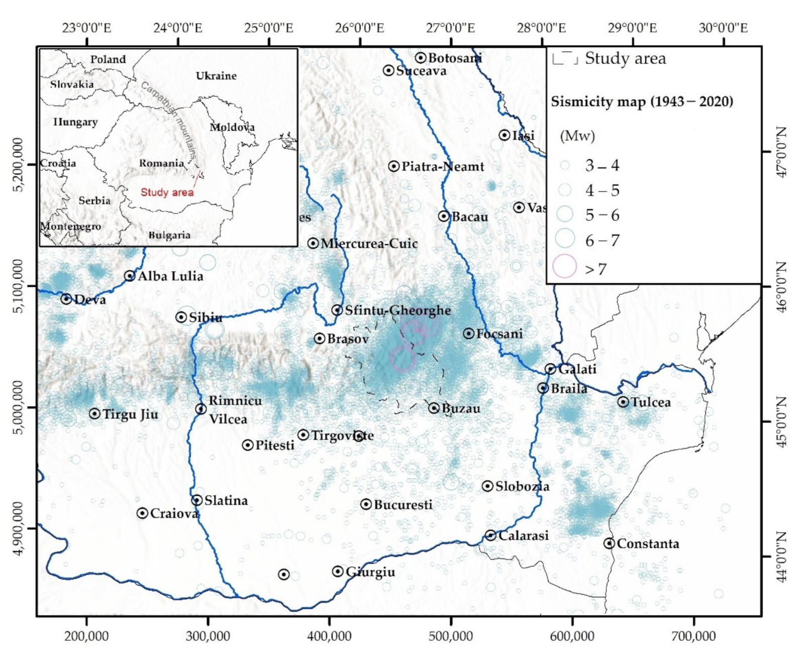
Figure 1. Seismicity map of Southeastern Romania and position of the study area: earthquake events marked in terms of moment magnitude M w (provided by NIEP, downloaded from the ArcGIS online server) and representation of the focal mechanisms of the events between 1943 and 2020 (USGS, 2021). Note, this map actually shows thousands of circles, each one corresponding to an event with a specific magnitude; their overlay locally produces the bluish colors, only the M w > 7 earthquakes appear as individual violet circles.
Geosciences 11 00495 g001
Figure 2. Position of the study area on the morphostructural units map of Romania (after Badea et al. [36], reproduced with permission from the authors). (A) The Carpathian Mountain, (a): Mesozoic-crystalline subunits; (a1): Eastern Massif; (a2): Southern Massif; (a3): Western Massif; (b): flysch subunits (b1): inner flysch; (b2): outer flysch); (c): volcano-sedimentary subunits (c1): Tibles-Bârgau Mountains; (c2): Metalliferous Mountains); (d): neovolcanic subunits (d1): Oaș-Gutâi-Văratec Mountains; (d2). Călimani-Gurghiu-Harghita Mountains); (e): intramontainous depressions (of tectonic or erosive origin). (B) Pericarpathian hills. (a1): Moldavian Subcarpathians; (a2): Curvature Subcarpathians; (b1): Getic Subcarpathians; (b2): Getic Piedmont. (C) The Intracarpathian Transylvanian Depression, (a): Someșan Plateau; (b1): diapiric folds sector; (B2): central domes sector. (D) Plain (a) and hills (b) of Banat and Crișana. (E) Moldavian Plateau. (F) Romanian Plain. (G) Dobrogea, (a): Northern Dobrogea; (b): Central Dobrogea; (c): Southern Dobrogea; (d): Danube Delta. (H) Boundary between orogenic and platform units. (I) (modified from Grecu [37]).
Geosciences 11 00495 g002
Figure 3. Landslide inventory. Inside the large blue rectangle, all landslides originate from Zumpano et al. [45] and Damen et al. [46] and were used for modelling and testing (about 10% of the landslides are reused for validation). Outside the rectangle, the landslides inventoried in the present study were used for validation. The landslide data have been used and are reproduced here with permission from the authors of both papers.
Geosciences 11 00495 g003
Figure 4. Earthquakes of magnitude greater than 7 (labels on the map), classified by depth, which occurred in and around the study area since 984. Based on data provided by NIEP through the ROMPLUS Catalogue [38].
Geosciences 11 00495 g004
Figure 5. Susceptibility maps for the landslide source zones (A) and for the runout zones (B), difference between the source density map and the runout density map (C), ROC curves used to evaluate the two susceptibility maps (D).
Geosciences 11 00495 g005
Figure 6. ND maps (cm) for saturation rate m = 1 , magnitude M w = 7.1 (depths D = 100   km (A), D = 150   km (B), D = 200   km (C)); magnitude M w = 8 (depths D = 100   km (D), D = 150   km (E), D = 200   km (F)).
Geosciences 11 00495 g006
Figure 7. Normalised probabilities for the ND map for saturation rate m = 1 , magnitude M w = 7.1   and depth D   = 100   km : (A) for the validation landslide inventory, (B) for the baseline landslide, (C) for both inventories, (D) for both inventories by combining the runout and the source zones.
Geosciences 11 00495 g007
Figure 8. Normalised probabilities for the ND map for saturation rate m = 1 , magnitude M w = 8   and depth D   = 100   km : (A) for the validation landslide inventory, (B) for the baseline landslide inventory, (C) for both inventories, (D) for both inventories by combining the runout and the source zones.
Geosciences 11 00495 g008
Figure 9. Comparison among: (A) source susceptibility zonation, (B) runout susceptibility zonation and (C) ND (in cm, saturation rate m = 1, magnitude M w = 7.1 and depth D = 100   km ) and (D) distribution of inventoried landslides on the shaded relief map.
Geosciences 11 00495 g009
Table 1. Climatic vertical zonation for Southeastern Romania [data from 41].
Type of ClimateAltitudes (m)Average Annual Temperatures (°C)Precipitation (mm/Year)
High mountain climate
Low mountain climate
Hill and plateau climate
>1700−2–21000–1100
800–17002–6850–1000
<300–8008–10500–850
Lowland climate
Climate of the seaside area
<20010–11450–600
>11<350–400
Table 2. Repression coefficients for the calculation of Ia (data from Foulser-Piggott and Goda [58]).
CoefficientIa (m/s)
C 0 1.786697
C 1 4.630313
C 2 1.106875
C 3 −0.592696
C 4 0.629011
C 5 −0.903888
Table 3. ND scenario maps produced in this study according to saturation rate, magnitude and depth of hypocenter.
ND ScenarioSaturation Rate
m
Magnitude
M w
Depth D
(km)
107.1100
207.1150
307.1200
408100
508150
608200
70.57.1100
80.57.1150
90.57.1200
100.58100
110.58150
120.58200
1317.1100
1417.1150
1517.1200
1618100
Table 4. Covariance matrix for ND maps (for magnitudes M w = 7.1 and M w = 8 with 100-km depth) as well as source and runout susceptibility maps (SS and AS).
MapND (7.1; 100)ND (8; 100)SSAS
ND (7.1; 100)0.526.190.090.03
ND (8; 100) 73.961.090.33
SS 0.070.05
AS 0.07
Table 5. Correlation matrix for ND maps (for magnitudes M w = 7.1 and M w = 8 with 100-km depth) as well as source and runout susceptibility maps (SS and AS).
MapND (7.1; 100)ND (8; 100)SSAS
ND (7.1; 100)1.00000.99980.47180.1352
ND (8; 100) 1.00000.47890.1424
SS 1.00000.7133
AS 1.0000
Publisher’s Note: MDPI stays neutral with regard to jurisdictional claims in published maps and institutional affiliations.