1. Introduction
In many shallow granular aquifers, groundwater levels show seasonal and interannual variability depending on natural and anthropogenic conditions. According to [
1], high groundwater levels may be related to the groundwater recharge potential (i.e., intense or long rainfall events, snow melt, high surface water levels, soil infiltration capacity, and soil saturation) and pressure transfer processes of the underlying groundwater reservoir. Anthropogenic measures that possibly contribute to elevated groundwater levels include sealing of surfaces, artificial groundwater recharge, or the building of runoff hydro power plants [
2]. In this context, extreme high groundwater levels are of concern, because they can lead to severe damages and economic losses due to flooding of basements, underground parking, waste dump sites, or other subsurface infrastructure [
3]. Thus, consultants and regulating authorities need information about extreme groundwater levels for project designs and land-use planning.
In surface hydrology, statistical frequency analysis is a standard tool to estimate discharge with a given return period or exceedance probability (e.g., [
4,
5]). In the subsurface, the objective is to relate the annual maximum groundwater levels to their frequency of occurrence through the use of an appropriate probability distribution [
1].
The estimation of extreme high groundwater levels should be based on groundwater level data at wells, which have been monitored for a sufficient long period (e.g., more than 30 years) and in an adequate frequency (e.g., at least once a week; [
6]). In that case, it is highly likely that high groundwater levels were not missed. Furthermore, the groundwater level at the location of the monitoring well should not be influenced by anthropogenic activities such as pumping, drainage, or recharge to be useful for estimation of extreme groundwater levels. If an influence exists, it should have been steady over the past years and also representative for future conditions. Additionally, groundwater level data have to be checked for a trend, and depending on the cause, it has to be decided if the trend should be removed prior to estimating the extreme high groundwater level data [
6].
Two of the most commonly used approaches in hydrological frequency modelling are the annual maximum series (AMS) approach and the peaks over threshold (POT) method [
4]. The AMS method considers only the annual maximum values regardless of whether the following events in one year exceed the annual maxima of other years (e.g., dry years). The POT method attempts to overcome these features by considering all events above a specified threshold level. Yet, appropriate threshold levels have to be defined to assure consecutive peak independence [
1]. At the beginning of the AMS approach, a suitable probability distribution is fit to a series of annual maximum peaks. Then, this distribution is used to estimate the groundwater level that is exceeded with a given probability or yearly return interval. Because the true probability distribution of the data is unknown, several probability distribution functions can be applied. The most commonly used probability distribution in AMS analysis is the generalized extreme-value (GEV) distribution [
1], which includes the Gumbel, Frechet, and Weibull formulations.
Reference [
7] applied four distributions in their regional frequency analysis study: generalized logistic distribution, Pearson type III distribution, 3-parameter lognormal distribution, and the extreme value type I Gumbel distribution. No general recommendation on a favorite distribution type could be derived. Reference [
1] compared six different estimates of groundwater levels with a 100 year return level using an AMS and a POT methodology, both with different parameter estimation methods. All combinations gave very similar estimates and standard deviations for the extreme groundwater levels so that no approach could be considered superior.
Reference [
6] regarded extreme groundwater levels computed with the Gumbel distribution as more plausible than results obtained with other distributions and estimation methods. Moreover, Gumbel-derived estimates were more robust against changes in the input data. Reference [
1] discussed that the two-parameter Gumbel quantile estimator could sometimes be preferable than a three-parameter GEV quantile estimator, even if the shape parameter is misrepresented. Because groundwater levels cannot exceed the local topographic elevation, [
1] applied the Gumbel procedure to avoid this upper bound inconvenience. Reference [
8] debated that in hydrology the double exponential, or Gumbel distribution, often approximates events in the upper tail of the distribution.
With respect to further approaches, [
9] combined statistical methods of hydrograph classification and lumped parameter models to simulate the spatiotemporal extent of groundwater flooding in a chalk catchment in southern UK. Reference [
10] combined statistical analysis of groundwater levels (clustered standardized indexes of groundwater flooding cross-correlated with standardized indexes of precipitation) and impulse response functions and revealed the overarching controls of groundwater flood response in the Chalk English lowlands.
Alternatively, extreme high groundwater levels can also be generated by driving a groundwater flow model with corresponding boundary conditions (e.g., combination of several successive wet years and the shutdown of well fields). Reference [
8] completed ensemble modelling of extreme groundwater levels due to climate change impacts and applied extreme value analysis (EVA) to projections of future extreme high groundwater levels (2081–2100). The authors computed groundwater levels for different return periods and compared differing sources of uncertainty. Reference [
2] ran a groundwater flow model with corresponding boundary conditions (higher recharge rate and elevated surface water levels) to derive a distribution of highest expected groundwater levels for the Berlin aquifer and compared the results with the highest measured groundwater levels at monitoring stations.
Yet, the determination of extreme groundwater levels at monitoring stations does not provide a continuous distribution over a groundwater body, which is needed for design and planning purposes. Thus, an interpolation step is needed that makes use of the extreme groundwater levels derived at neighboring stations. References [
7,
11] applied ordinary kriging in that context. However, interpolation between the point extreme estimates lacks the ability to account for the impact of natural conditions (e.g., drainage of groundwater by surface water bodies) or anthropogenic uses (e.g., groundwater withdrawal) between monitoring wells on the distribution of groundwater extreme values. This information is provided by regional and transient groundwater flow models that, given high calibration quality, well represent the impact of natural conditions and anthropogenic uses of the aquifer on groundwater levels.
In the approach presented herein, a novel methodology for estimating a distribution of extreme high groundwater levels is introduced where the Gumbel is the applied method to estimate local extreme high groundwater levels from groundwater level time series simulated at each node of the computational mesh of a groundwater model. Given a 25-year simulation period, a return period of 100 years was selected, i.e., extreme groundwater levels, that are reached or exceeded once in 100 years. Furthermore, a correction step was implemented that accounts for the influence of the imperfect representation of the observed groundwater levels by the simulated time series on the estimation of the groundwater levels with a hundred year return period (GLsWHYRP) at the observation wells. Thus, distributions of GLsWHYRP between monitoring wells are made available on a physical basis. Finally, we applied the approach to compute the distribution of GLsWHYRP based on a model scenario where all groundwater withdrawals were shut down in the example aquifer.
3. Results
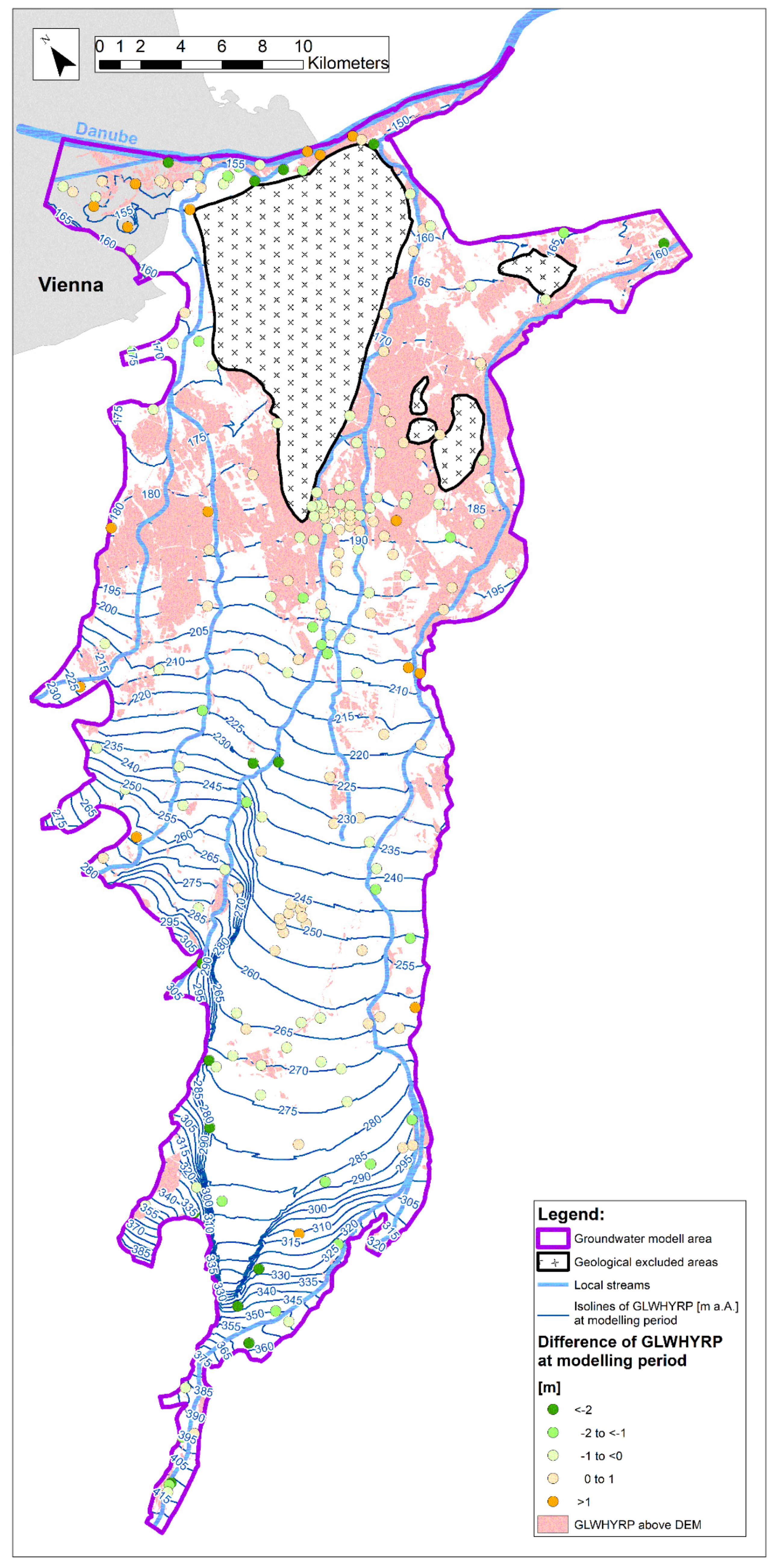
In
Figure 3, the isolines of GLsWHYRP in the SWB aquifer based on the application of the Gumbel approach at each finite element node is shown. It can be seen that the general flow pattern (i.e., main flow direction from the southwest to the northeast and the steep gradients in the southwest part of the model domain) are kept compared to the median groundwater level distribution shown in
Figure 1. The salmon color areas show regions where the predicted GLsWHYRP exceed the ground surface. These areas correspond well to regions where the median groundwater level is only between 1 m to 2 m below the ground surface (see also [
16]). Furthermore,
Figure 3 includes the differences between the GLsWHYRP computed based on the modeled and on the observed groundwater level time series at the observation wells in the simulation period. Maximum deviations range from an underestimation of about 4 m (green colored dots) to an overestimation of about 1.5 m (orange colored dots) by the model-derived GLsWHYRP. This means that using the simulated annual maximum groundwater levels mostly results in lower estimations of GLsWHYRP at the observation wells in the SWB aquifer. In general, over- and underestimations are both spread over the entire aquifer, though the number of observation wells showing underestimations is higher than that of overestimations.
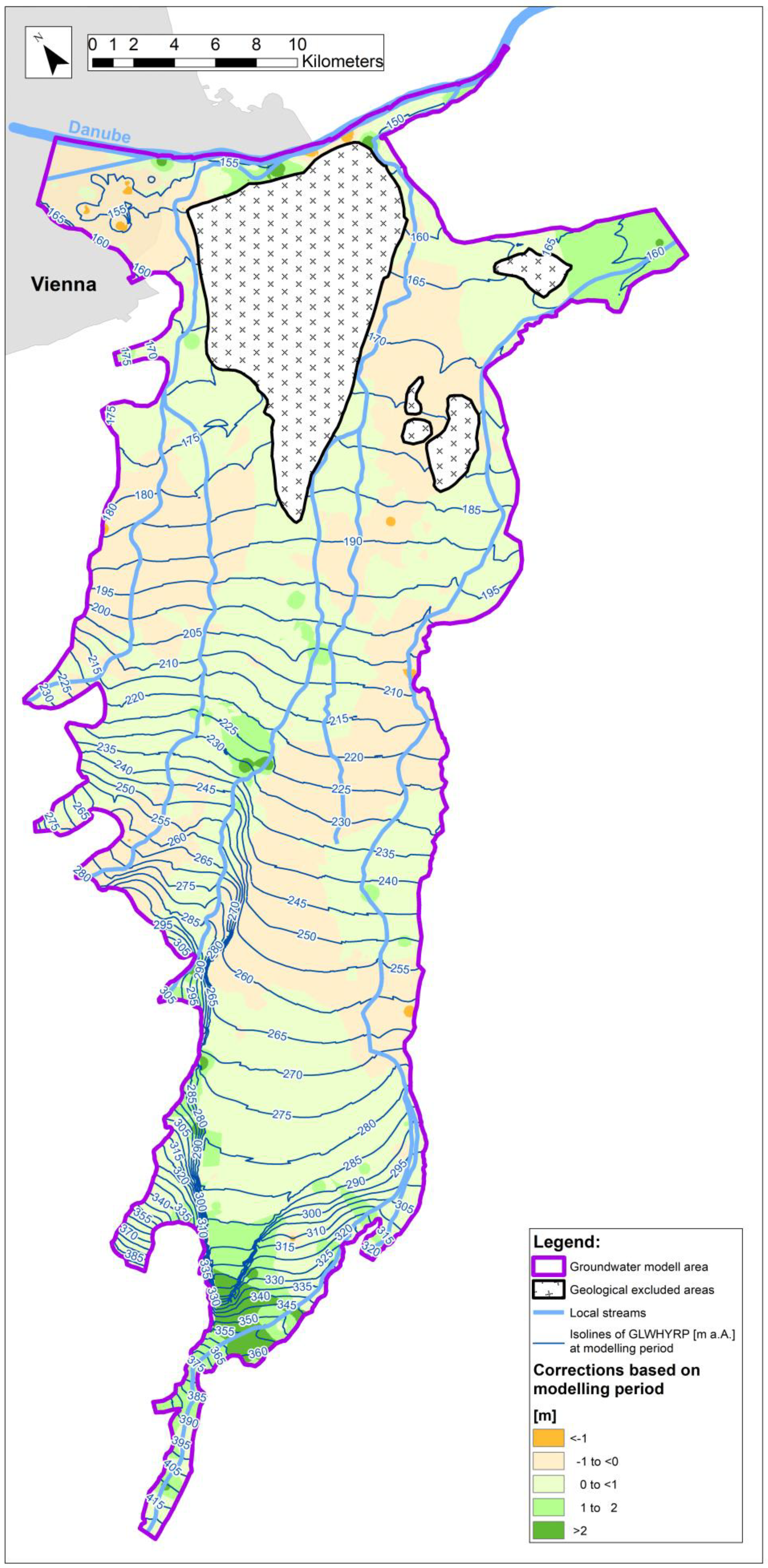
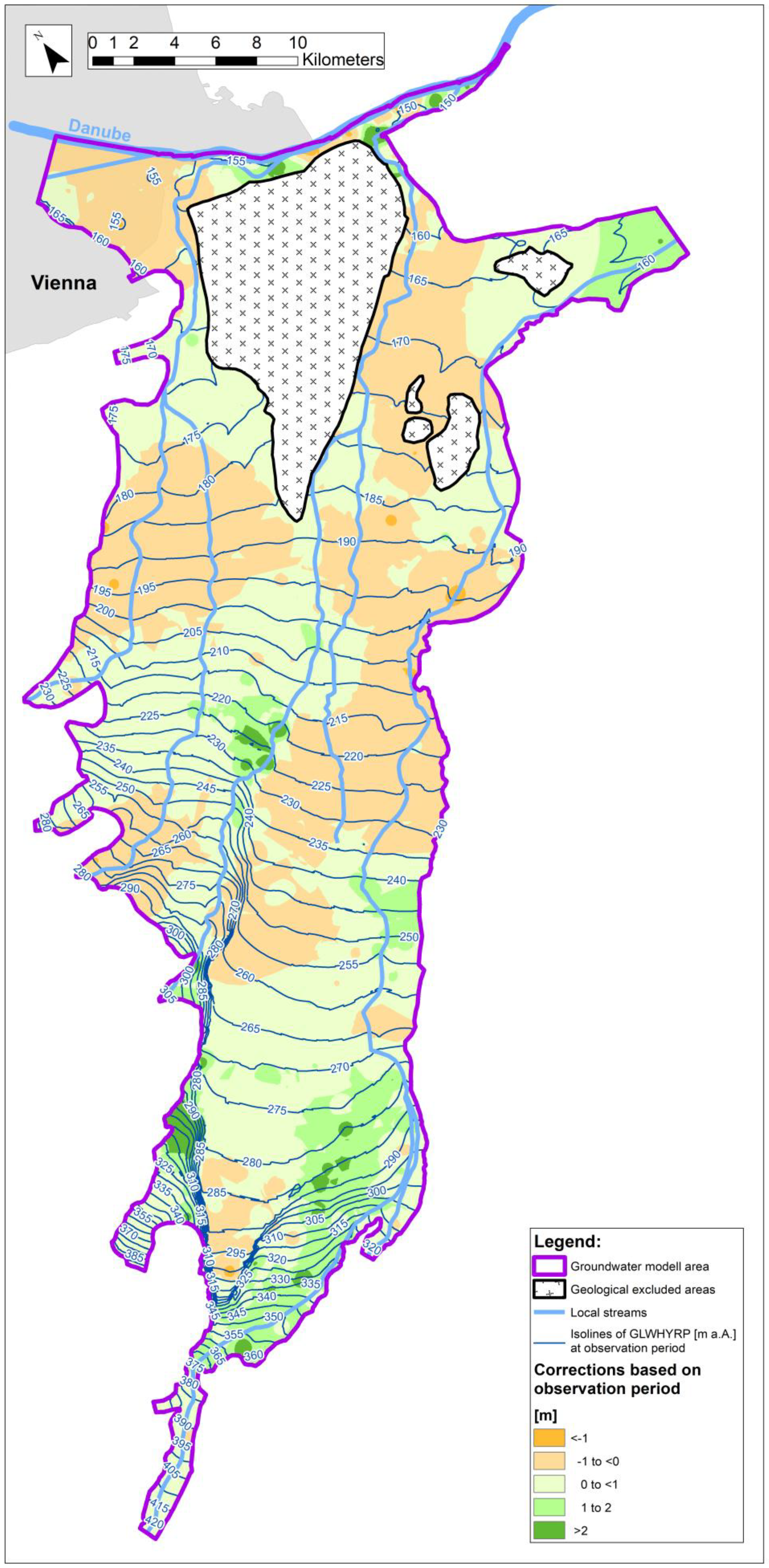
In
Figure 4 the GLWHYRP isolines are shown that include the interpolated corrections, which reflect the discrepancies between the model- and observation-based GLsWHYRP at the observation wells in the simulation period. Additionally, the interpolated corrections that are added to the model-based GLsWHYRP are displayed in
Figure 4. For the interpolation, ordinary kriging was used applying an isotropic search radius of 5000 m and using at least three and at maximum five neighboring correction values. Fitting of the corresponding experimental variogram was completed with 25 lags of 200 m each.
Most of the model area shows corrections which fluctuate between −1 m and 1 m; larger corrections result only locally. The highest corrections result in the southern part of the SWB aquifer, where the step fault induces large groundwater gradients. Overall, the distribution of corrections in
Figure 4 shows no systematic bias. It has to be noticed that the corrections in
Figure 4 inversely correspond to the point differences shown in
Figure 3, i.e., if the model-based GLWHYRP is lower than the observation-based GLWHYRP at an observation well the correction applied to the model-based GLWHYRP must be positive.
Figure 5 depicts the GLWHYRP isolines that include the interpolated corrections, which were derived using the longest possible observation period at every observation well given the observations comply with statistical criteria to apply the Gumbel approach. As in
Figure 4, the interpolated corrections that are added to the model-based GLsWHYRP are shown in
Figure 5. Comparing the distribution of corrections between
Figure 4 and
Figure 5, it can be seen that in general the use of the longer observation period leads to larger reductions (dark beige colored areas) of the GLsWHYRP in relevant areas of the downstream part of the SWB aquifer, whereas the opposite is true for most of the upstream part of the aquifer. Near the step fault in the upstream aquifer, the largest differences exist if the corrections are computed using the model simulation period or the total observation period to derive the GLsWHYRP at the observation wells. This is mainly due to the combination of large groundwater level fluctuations and the steep groundwater gradient near the step fault.
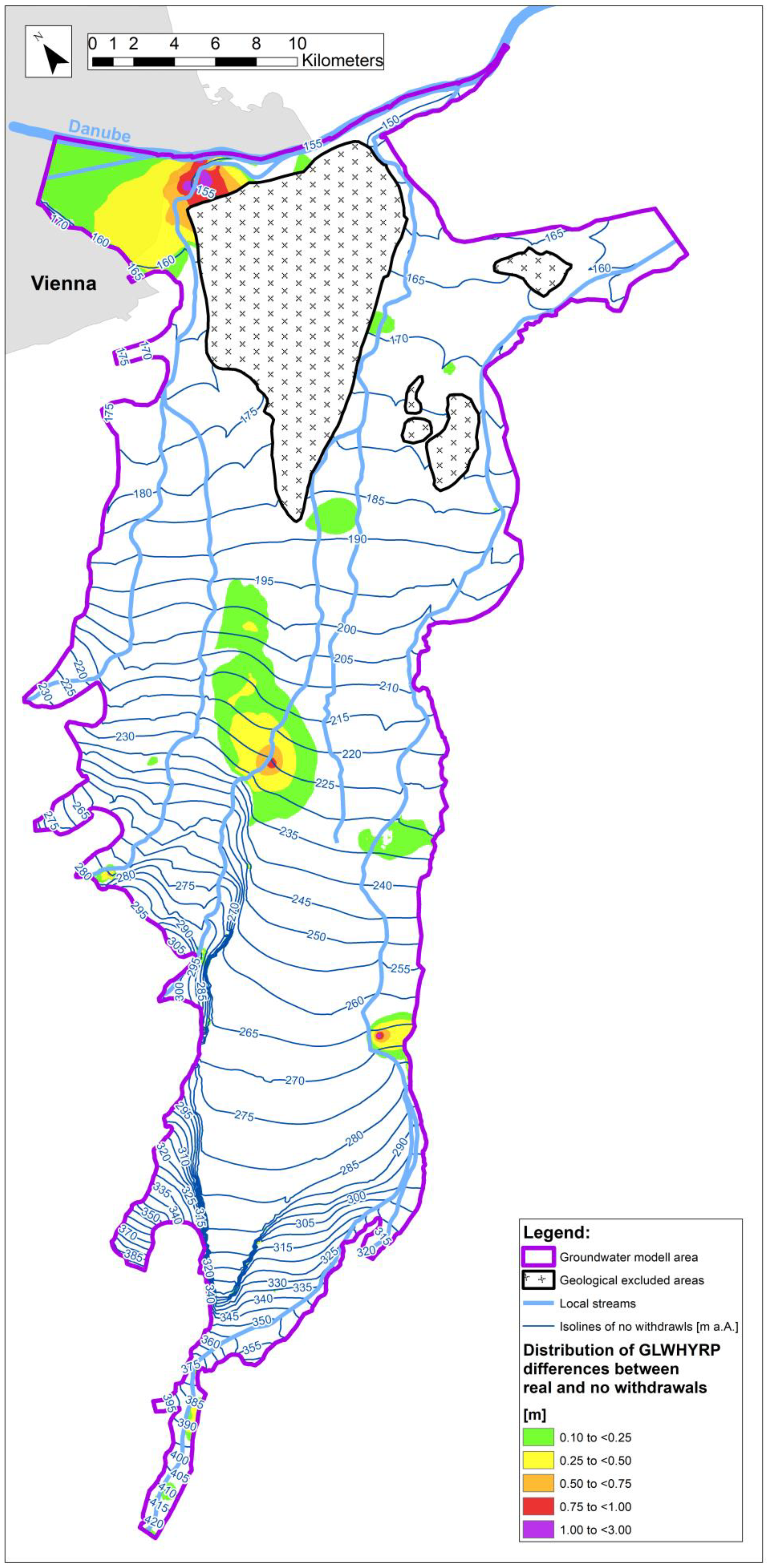
Figure 6 shows GLWHYRP isolines that result if the Gumbel approach is applied to groundwater level time series for a modeling scenario with no groundwater withdrawals in the simulation period. Moreover, the differences between the GLWHYRP distributions for the real pumping schemes and for no groundwater withdrawal are included in
Figure 6. To be methodically consistent, for this comparison no correction was applied to the GLWHYRP distributions of the real pumping schemes, since a correction cannot be computed for the scenario due to non-existing observations. It can be seen that though groundwater withdrawal wells are spread over the entire model area only a few pumping wells affect the yearly groundwater peak values that determine the estimation of GLsWHYRP. Maximum increases in GLsWHYRP are around 1 m if pumping wells are shut down and need to be considered if local assessments of peak groundwater levels are required.
4. Discussion
To avoid the shortcomings of interpolating peak groundwater values to generate a distribution of very high groundwater levels we applied extreme value analysis to the simulated groundwater level time series at each mesh node of a numerical groundwater model. Hence, all influences on the groundwater level (including natural and anthropogenic causes) are considered in an appropriate spatial and temporal manner to estimate peak groundwater values. Specifically, we employed the Gumbel approach to simulated groundwater level time series over 25 years in the SWB aquifer south of Vienna and computed the distribution of peak groundwater levels with a return period of a hundred years. This procedure also entails that the estimation of groundwater extreme values is based on exact the same time period, which is typically not the case because groundwater level time series at observation wells may show diverging observation periods. Thus, the homogeneity of the resulting distribution of GLsWHYRP will be improved. Moreover, the general procedure is not limited to the application of the Gumbel approach to estimate groundwater extremes with a given return period. Other methods of extreme value analysis in the context of peak groundwater levels, such as those discussed in [
7], could be implemented as well.
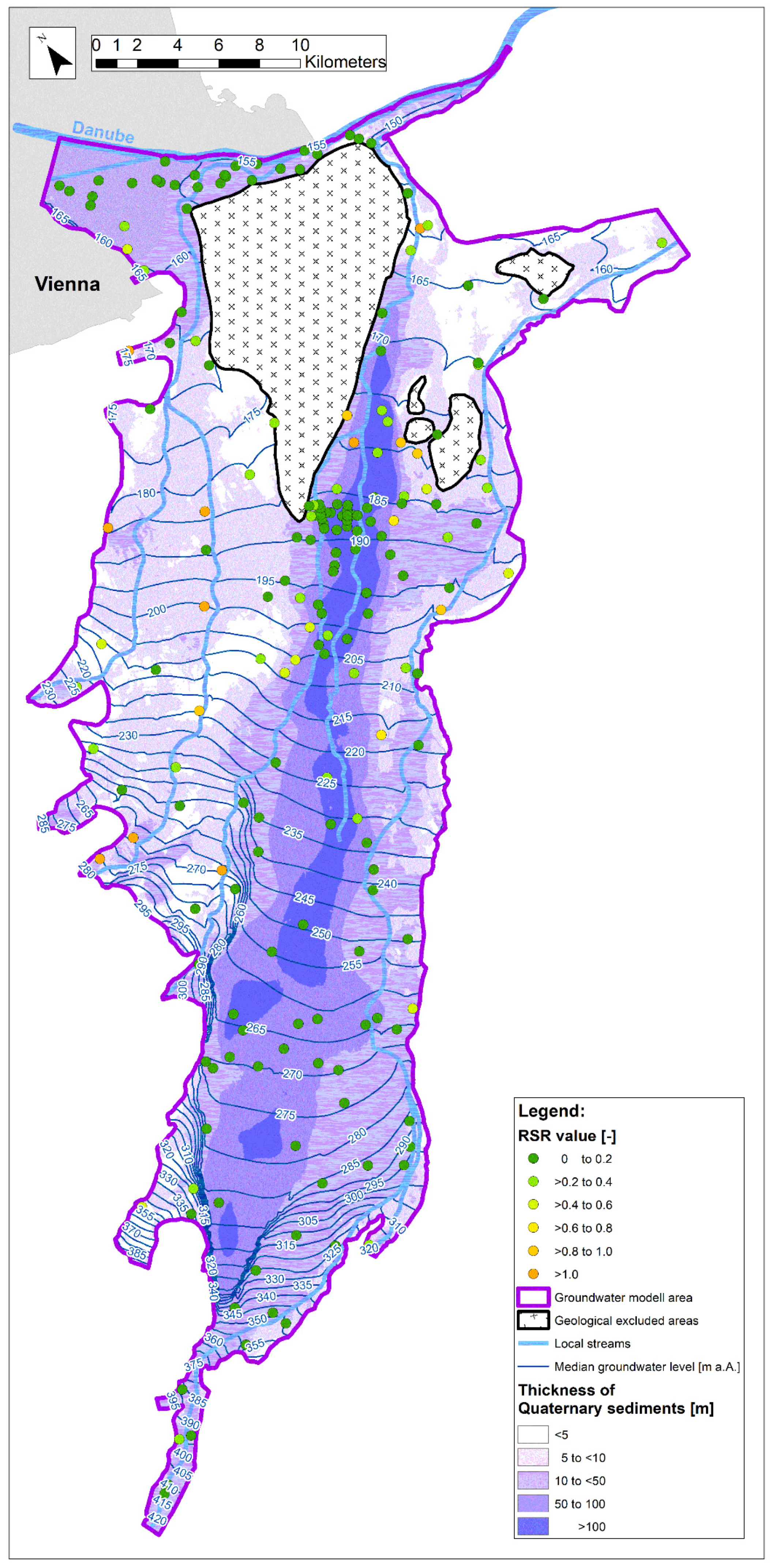
Though groundwater models are evaluated against the reproduction of observed groundwater levels, model results are still uncertain due to simplifications during the model setup process and incomplete knowledge about parameter distributions. Most often in the calibration of multiyear groundwater models less priority is devoted to the reproduction of peak groundwater levels. However, these values are essential to extreme value analysis methods. Thus, it is to be expected, that at the location of the observation wells the estimated extreme groundwater levels based on simulated groundwater levels and on observed groundwater levels will differ. Yet, these differences are not to be mixed with the overall calibration quality of the groundwater model. Several targets can be used in the definition of the objective function during the model calibration and different measures for calibration quality may be applied. For the SWB aquifer, we used the root mean squared error standard deviation ratio to account for the large fluctuations of the groundwater level during the 25-year simulation period. Other error measures are discussed, e.g., in [
19,
20]. Thus, calibration quality measures (like the Nash–Sutcliffe efficiency or the RSR) can only provide a first indication of the discrepancies between model- and observation-based estimates of GLsWHYRP at observation wells.
In that context, ref. [
7] state that groundwater flow models have their limitations when considering extreme conditions and do not give insights into probabilities and return periods. By the described workflow, we have shown a combination of local extreme value analysis with groundwater model results that generate a regional distribution of extreme groundwater levels without a homogeneity assumption. In general, we expect high benefits from the combination of extreme value analysis and groundwater model results in inferring distributions of peak groundwater levels in aquifers that have distinct hydraulic features due to specific hydrogeological, hydraulic, or anthropogenic conditions that cannot be adequately captured by interpolating locally derived estimates of extreme groundwater levels.
Comparing model- and observation-based estimates of the GLsWHYRP in the SWB aquifer, no systematic bias can be observed; however, number and absolute values of underestimation by model-based estimates of GLsWHYRP are higher than those in cases of overestimation. In regions with little or no influence from surface water bodies, peak groundwater levels do not show short-term extreme variations and can be easier met by groundwater model results; thus, it is likely that in such cases the model-based estimates of GLsWHYRP are closer to observation-based values. Overestimation of observation-based estimates of GLsWHYRP can be expected if the modeled groundwater levels exceed the observations for high and low groundwater levels.
To consider the differences between GLsWHYRP based on simulated and observed groundwater levels at observation wells, we interpolated these discrepancies over the entire model domain and added the corrections to the GLsWHYRP based on simulated groundwater levels at the model nodes. Hence, the interpolation is limited to the differences between model- and observation-based estimations of groundwater peak values at the observation wells, which is in contrast to the interpolation of the estimated groundwater peak values if no groundwater model results are available. The needed corrections are smaller the closer the fit between observed and simulated groundwater level time series with respect to groundwater peak values.
Furthermore, we analyzed the effect of limiting the observations of groundwater levels to the simulation period of the groundwater model instead of using all available groundwater level observations to estimate the peak groundwater levels at the well locations. For the characteristics of the SWB aquifer, it turned out that the GLsWHYRP estimated on the basis of the simulation period between 1993 and 2017 is higher in the downstream part of the aquifer, where draining conditions dominate, by an average margin of about 0.2 m and lower in the upstream part of the aquifer, where recharging conditions prevail, by an average margin of about 0.4 m.
Obviously, it is to be expected that with an increasing length of the observation period the likelihood of a larger spread between annual groundwater peaks rises. The resulting differences between estimates of GLsWHYRP based on simulated and observed groundwater levels can be regarded small compared to the observed fluctuations of annual groundwater peaks of up to 10 m at some observation wells in the SWB aquifer. This means that the annual maximum groundwater levels in the simulation period are representative of peak groundwater levels in the previous years with respect to the estimation of the GLsWHYRP. This condition might be different in other groundwater bodies so that the sufficient length of the groundwater model simulation period to provide robust estimates of GLsWHYRP needs to be assessed for each groundwater body separately.
Based on the inherent characteristics of the AMS approach also years with below-average groundwater levels are considered to delineate the sample of high groundwater levels that is being used to estimate extreme groundwater levels with a given return period. This leads to an increased spread of the values in the sample, which causes in turn higher estimates of the extreme groundwater value independent of the probability distribution used.
To test the effect of this finding on groundwater level extreme estimates, the PoT approach was also applied to define the sample for the extreme value analysis. It turned out that the difference between GLWHYRP estimates based on the two approaches becomes most noticeable for groundwater level time series that show little short term fluctuations but are dominated by long periods of groundwater decline. Observation wells with such features are concentrated in a restricted area at the western model boundary of the SWB aquifer and affect only about 3% percent of the total amount of groundwater level time series. Thus, it was concluded to prefer the unambiguous procedure of the AMS approach for the delineation of the extreme value analysis sample over the application of empirical regulations in defining groundwater level extremes and of selecting effective thresholds within the PoT approach.
We also applied the developed procedure to the Westliches Leibnitzer Feld aquifer in the Province of Styria, Austria. Details about hydrogeological conditions and the development of the groundwater flow model can be found in [
21,
22]. Reference [
7] computed extreme groundwater level distributions in the same aquifer by regional frequency analysis after classification of observation sites into groups with homogeneous site characteristics and hydrological properties. The authors conclude that in aquifers, where disturbances of the natural groundwater regime had occurred (e.g., hydropower constructions, pumping), major parts of the aquifer could not be assigned to a statistically homogeneous region for regional frequency analysis. Thus, the uncertainty of the estimated quantiles of the probability distribution at the observation points increases. In this respect, the presented approach is more robust, since effects of groundwater level disturbances are handled by using simulated groundwater level time series to estimate groundwater level extremes.
Additionally, the entire estimation procedure can be applied to estimate the distribution of extreme low groundwater levels with a selected return period, which we completed for the Westliches Leibnitzer Feld aquifer. In that case, the extreme value analysis will be based on observed annual low groundwater levels. The related correction at the location of the observations wells will then mainly depend on the reproduction of observed groundwater lows by the simulated groundwater level time series. Thus, extreme high and low groundwater levels are available for use in operation and construction design.
By involving a groundwater model in estimating regional extreme groundwater level distributions assumptions about future land use or different hydrological boundary conditions can be processed into results of model scenarios, which can be further used as a basis to infer maps of peak groundwater values with a selected return period. For the SWB aquifer, we investigated the impact on the GLWHYRP distribution if all groundwater wells would be shut down. In particular, it was of interest if the areas, where the groundwater extreme levels reach or exceed the ground level, will increase significantly compared to the current conditions. The corresponding map of differences between the isolines of estimated GLsWHYRP based on the real withdrawal case and on the no-withdrawal scenario clearly shows regions where the GLsWHYRP are most sensitive to the withdrawal stop. This information can be useful for planning of future land use or infrastructure measures. In that context, the groundwater model could also be driven by boundary conditions that are delineated from projection of future changes in the temperature and precipitation regimes and thus provide a systematic approach to quantify the impacts of global change on extreme groundwater levels (highs and lows due to wet and dry conditions) with a given return period.
5. Conclusions
The knowledge about extreme high groundwater levels is needed for planning purposes to avoid structural and environmental damage by groundwater flooding. Peak groundwater levels can be calculated by applying extreme value analysis methods to sufficiently long observed groundwater levels.
Groundwater models at the aquifer scale comprise all available knowledge about hydrogeological characteristics and hydraulic boundary conditions (including natural and anthropogenic causes) in a physical consistent and highly resolved manner. To avoid the shortcomings of interpolating peak groundwater values, we developed a methodology where the groundwater level with a hundred year return period is calculated by the Gumbel distribution at each node of a numerical groundwater flow model. In comparison to existing approaches to regionalize extreme groundwater levels, no further assumptions (e.g., homogeneity) are needed.
The methodology was applied to the SWB aquifer south of Vienna where a groundwater model with a 25-year simulation period is available. At the observation wells the GLsWHYRP based on the model results were compared to the values obtained by using the groundwater level observations. The resulting discrepancies are related to the fact that most groundwater models show limitations in reproducing groundwater extreme values though the calibration quality over the total simulation period is satisfying. To account for these circumstances, the discrepancies between model- and observation-based GLsWHYRP are interpolated across the model domain and added as corrections to the nodal GLsWHYRP. For the SWB aquifer, we could show that most of the downstream part will be inundated by the groundwater level with a hundred year return period, which is an important information for spatial planning purposes.
At many observation wells in the SWB aquifer groundwater level, data were available prior to the begin of the simulation period of the groundwater model. To test the effect of this additional data on the distribution of GLsWHYRP, we calculated the discrepancies between simulation- and observation-based GLsWHYRP using all available readings for the latter. In the SWB aquifer the resulting distributions of GLsWHYRP differ only between 0.2 m and 0.4 m, meaning the simulation period is representative of the longest available observation period at any observation well with respect to estimating the GLsWHYRP. This condition has to be individually tested for each groundwater body, because in general, a higher estimate of an extreme groundwater level is more likely in a longer evaluation period.
Large benefits with respect to computing the distribution of GLsWHYRP can be anticipated in groundwater bodies that show distinct hydrogeological features or anthropogenic impacts. The same overall procedure can be used to calculate extreme groundwater low levels if the safety of a water supply from groundwater resources needs to be assessed. The groundwater model can also be applied to run scenarios about groundwater use or changing boundary conditions to quantify the corresponding effects on the distribution of extreme groundwater levels. In that context, we identified most sensitive areas for an increase in GLsWHYRP if groundwater withdrawals will be ceased.


