Simulation of Broadband Ground Motion by Superposing High-Frequency Empirical Green’s Function Synthetics on Low-Frequency Spectral-Element Synthetics


Abstract
1. Introduction
1.1. Source Model Selection
1.2. Low-Frequency Ground Motion Waveforms
1.3. High-Frequency Ground Motion Waveforms
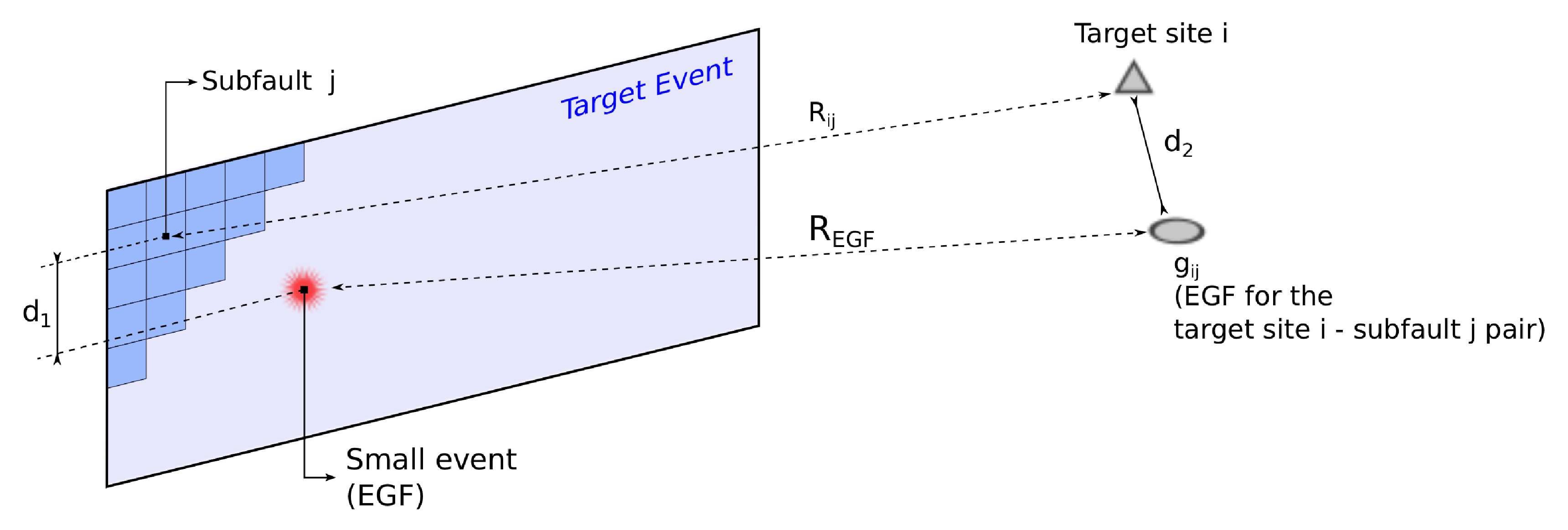
1.3.1. EGF Event Selection
- E: Closeness measure
- : Distance between the target site i and the centroid of the subfault j
- L: Length of the fault in the strike direction
- : Distance between the EGF hypocenter and the centroid of the subfault j (in 3-D space)
- : Distance between the seismic station and the target site i (in 3-D space)
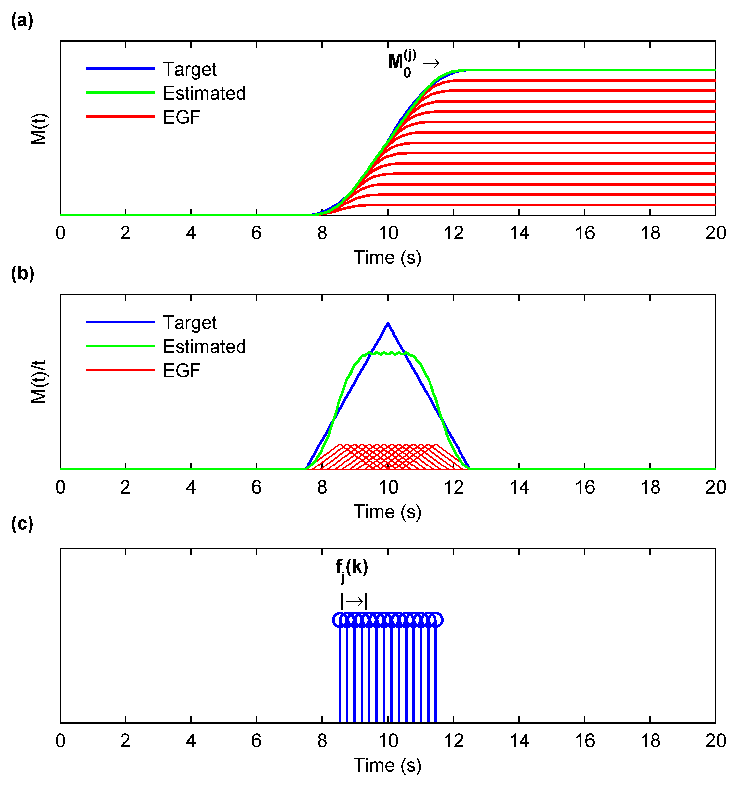
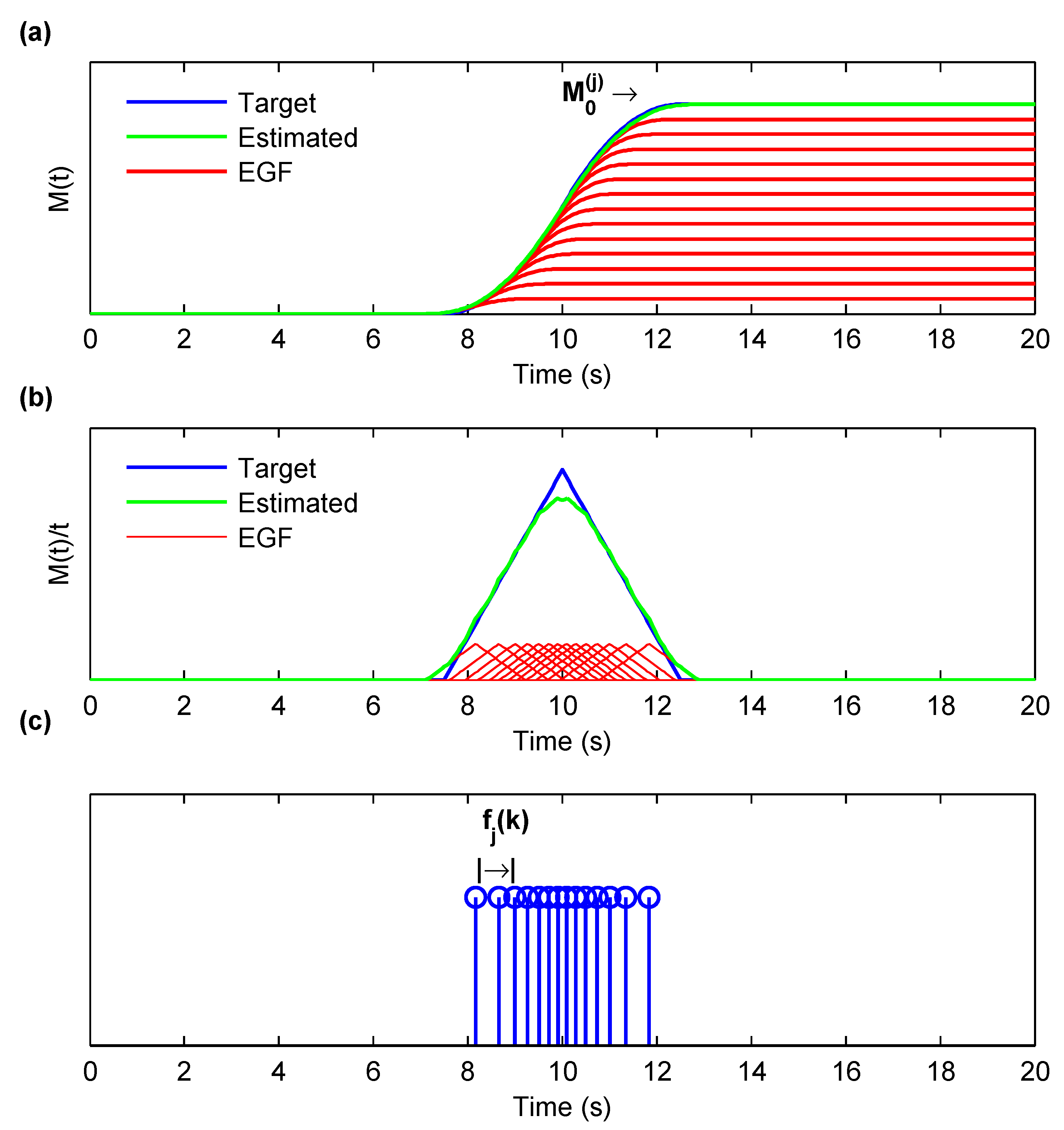
1.3.2. EGF Summation
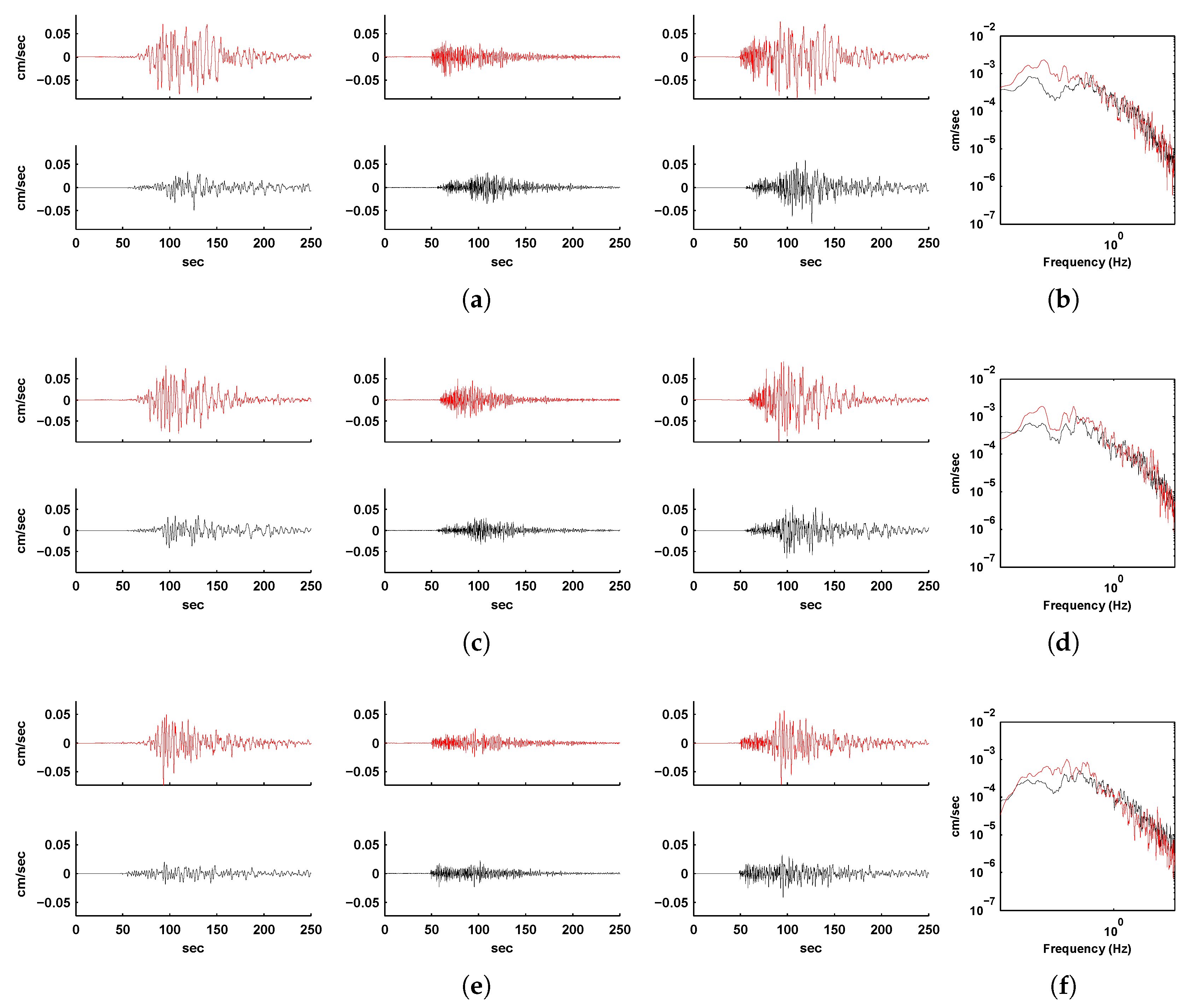
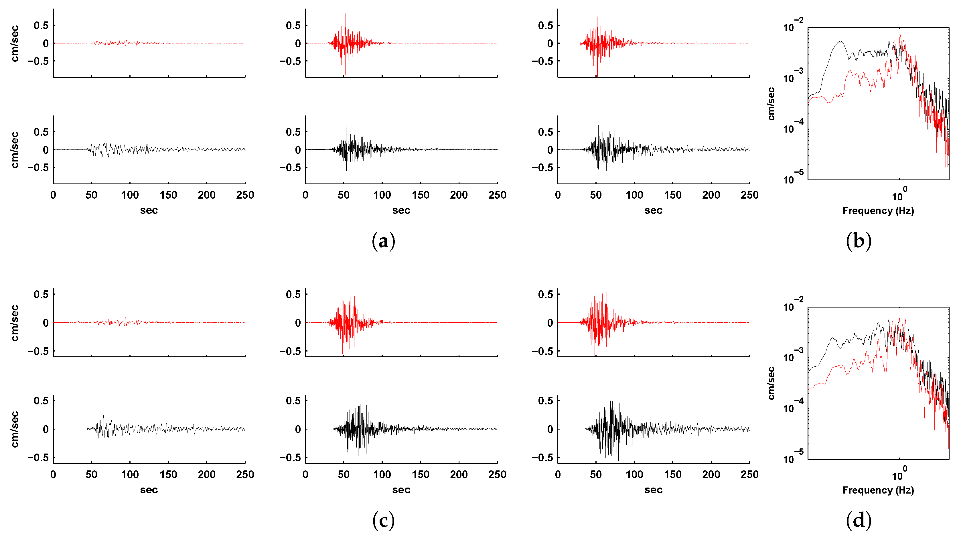
2. Validation of Methodology
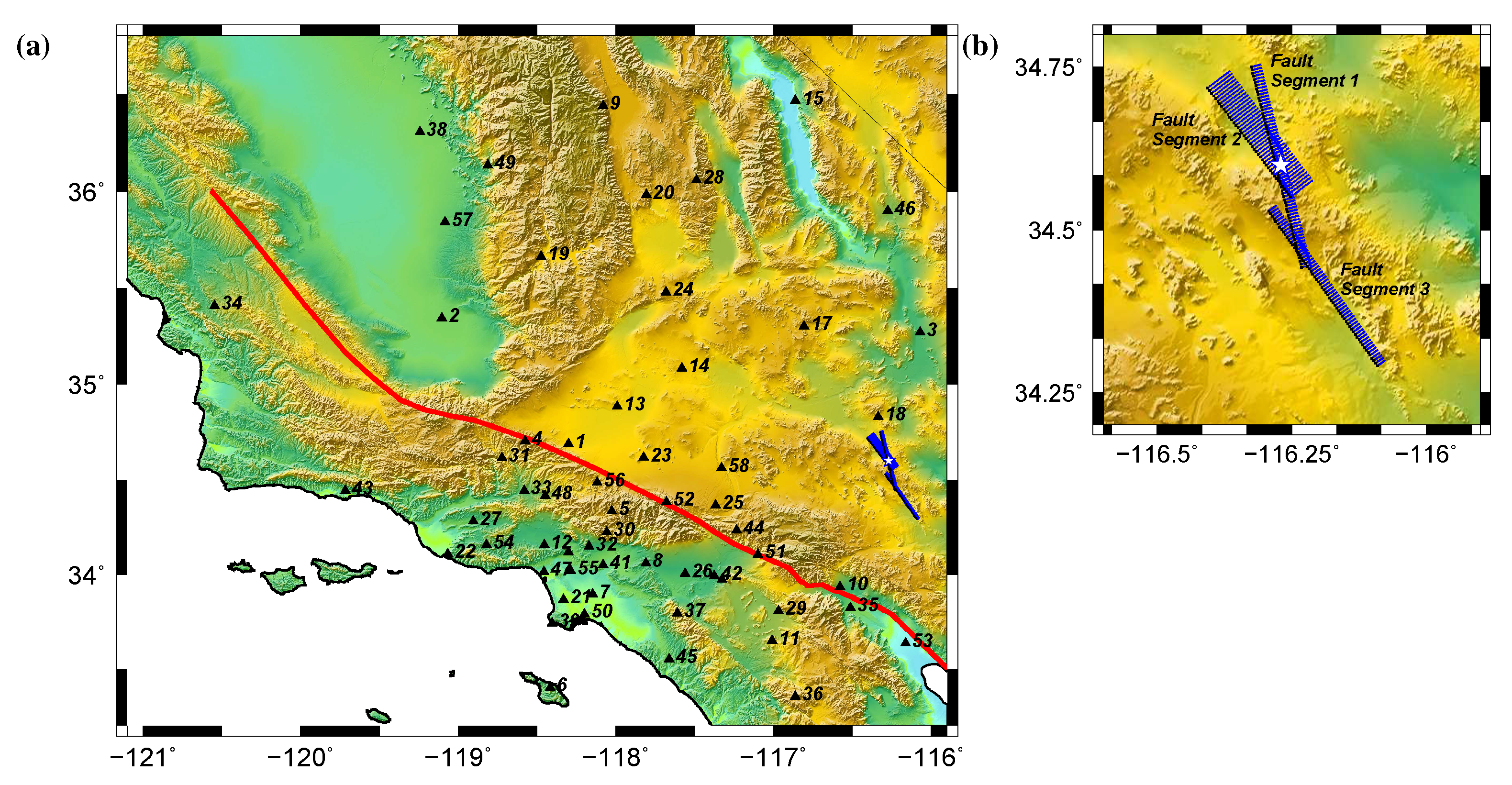
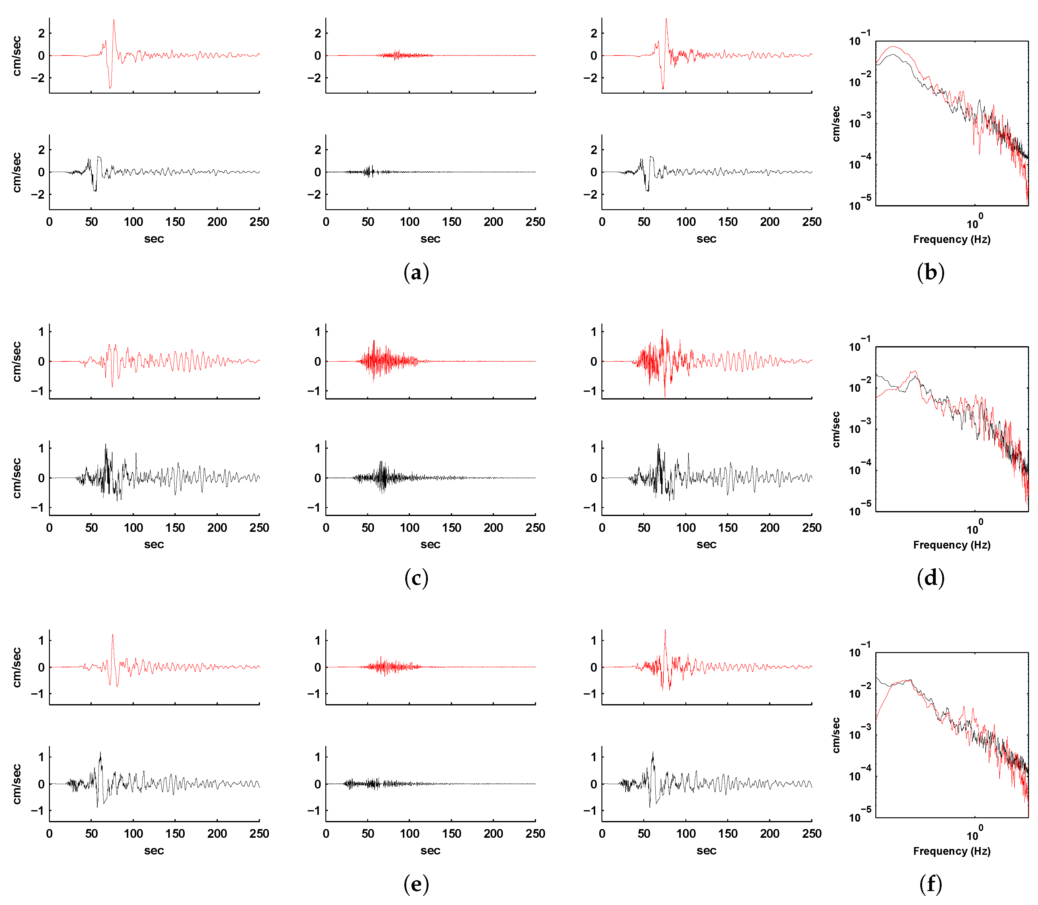
2.1. Validation 1: 1999 7.1 Hector Mine Earthquake
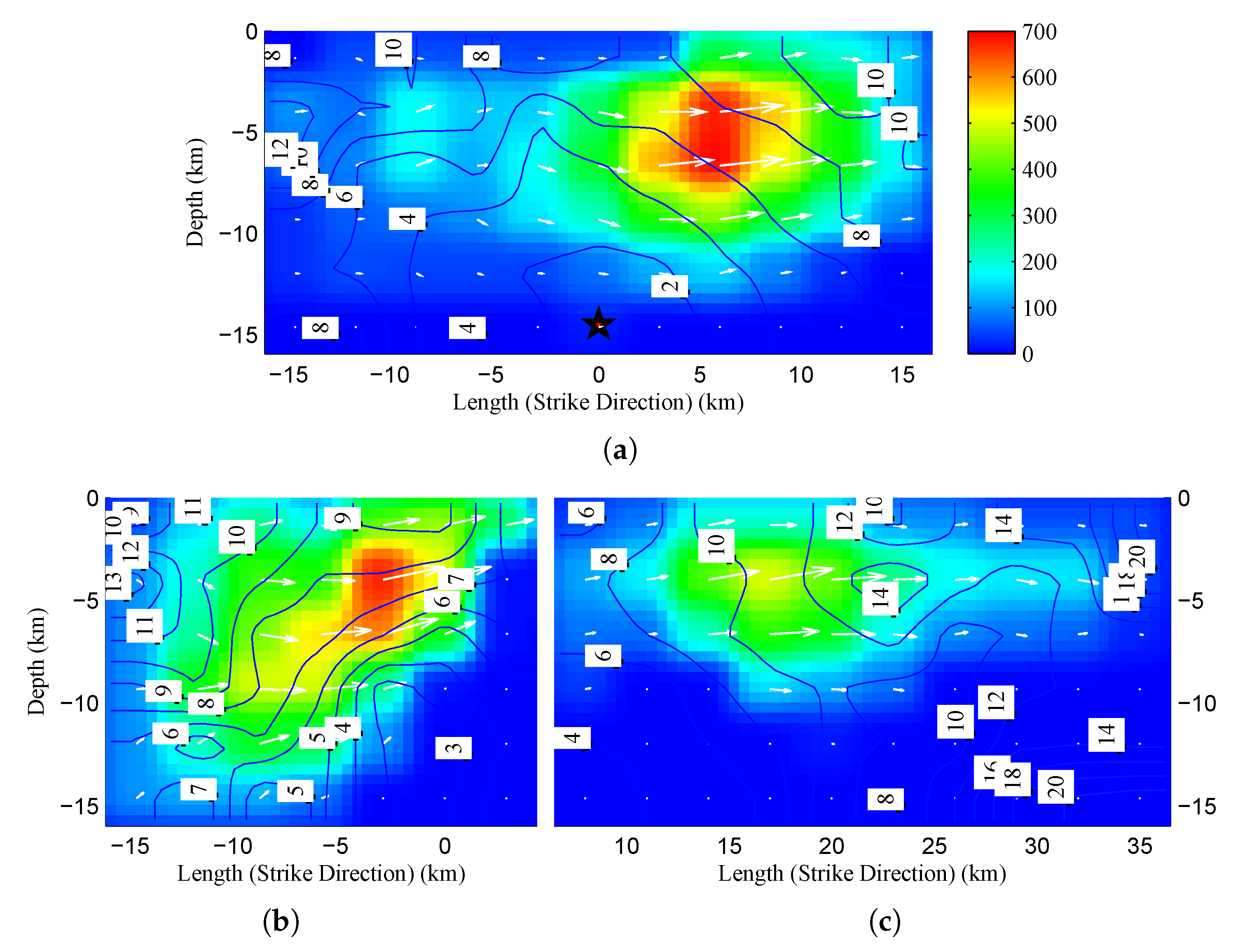
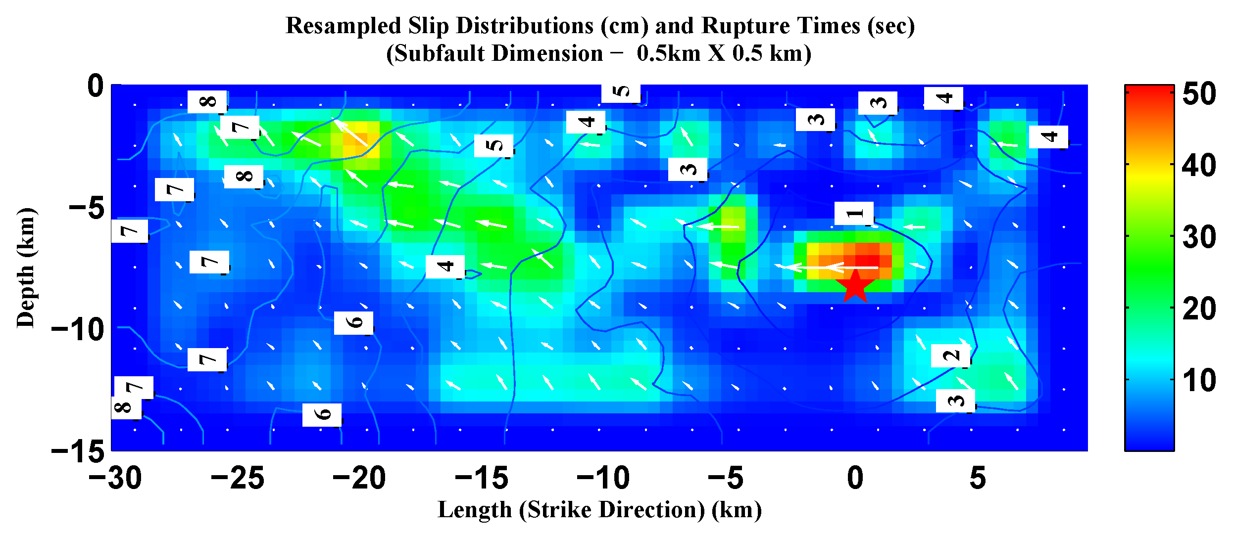
Source Model
- (i)
- and , respectively, for the northern segment,
- (ii)
- and , respectively, for the central segment, and
- (iii)
- and , respectively, for the southern segment.
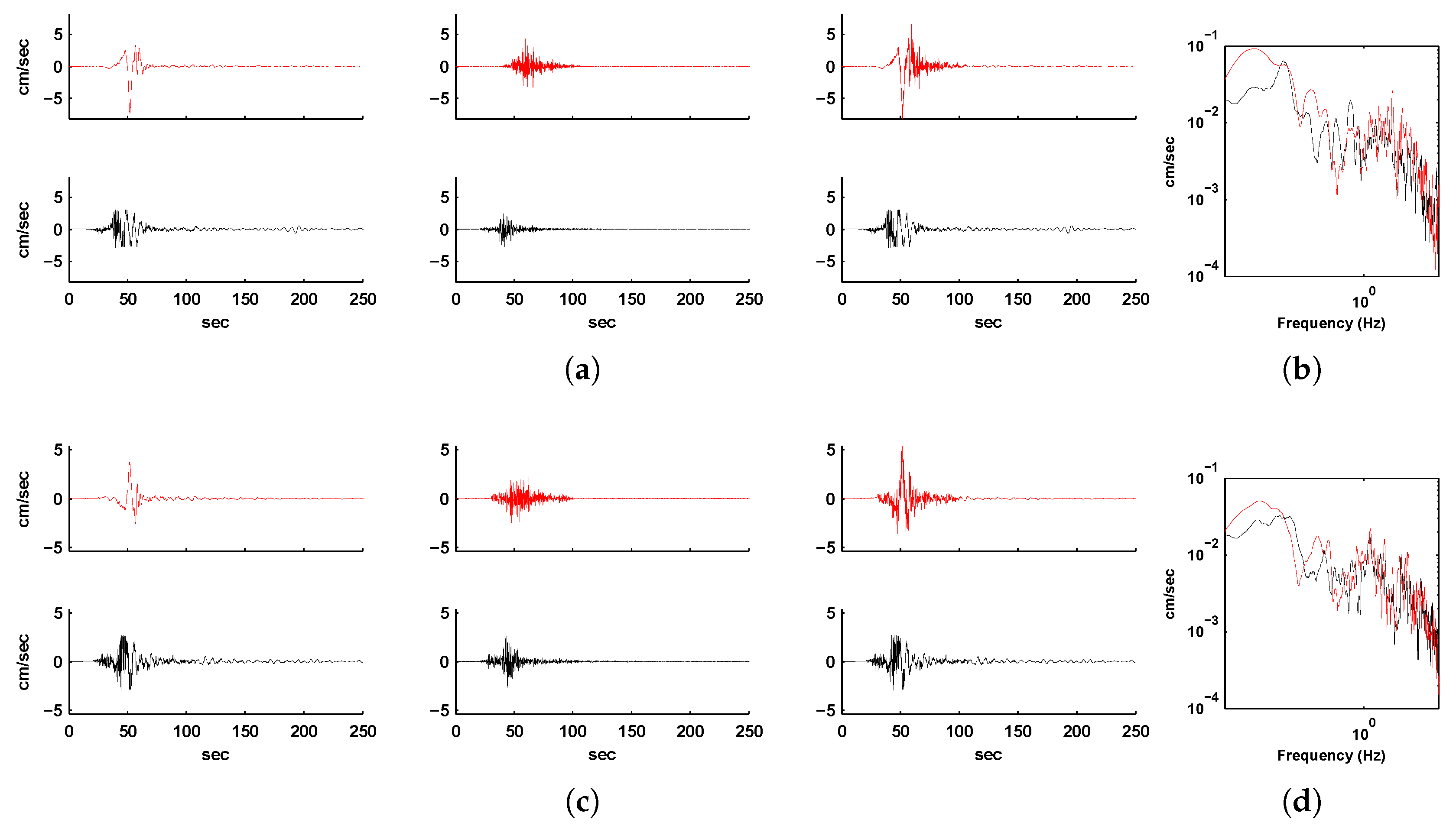
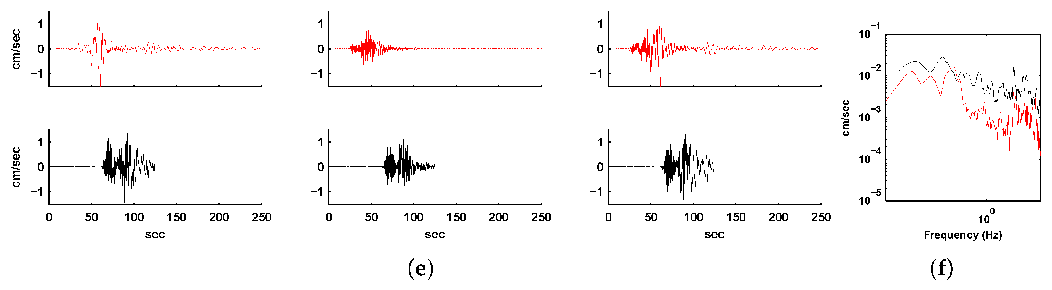
3. Validation 2: 2004 6.0 Parkfield Earthquake
4. Discussion
5. Conclusions
Author Contributions
Funding
Acknowledgments
Conflicts of Interest
Abbreviations
| EGF | Empirical Green’s Function |
| SCEC | Southern California Earthquake Center |
| CVM | Community Velocity Model |
| SCEDC | Southern California Earthquake Data Center |
| STP | Seismogram Transfer Program |
| PGV | Peak ground velocity |
Appendix A
Appendix A.1. Bias in Synthetics Associated with Sa
Appendix B
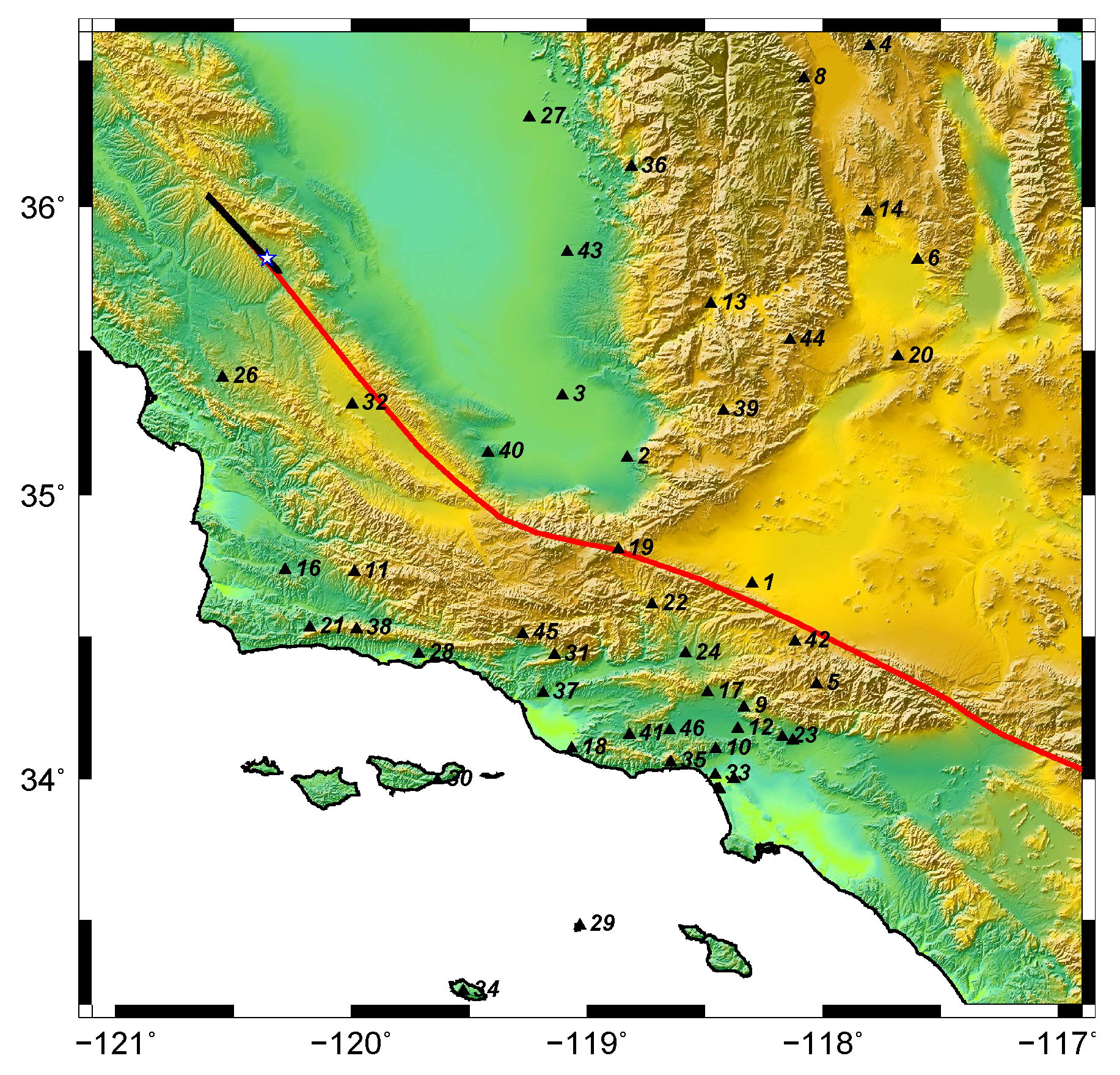
Appendix B.1. List of Stations

| Station Number | Latitude | Longitude | Location | Station |
|---|---|---|---|---|
| 1 | 34.68708 | −118.29946 | Antelope | ALP |
| 2 | 35.26930 | −116.07030 | Baker | BKR |
| 3 | 34.68224 | −118.57398 | Burnt Peak | BTP |
| 4 | 34.33341 | −118.02585 | Chilao Flat Rngr. Sta. | CHF |
| 5 | 33.40190 | −118.41502 | Catalina Island Airport | CIA |
| 6 | 34.06020 | −117.80900 | Cal Poly Pomona | CPP |
| 7 | 33.93597 | −116.57794 | Devers | DEV |
| 8 | 33.65001 | −117.00947 | Domenigoni Reservoir | DGR |
| 9 | 34.10618 | −118.45505 | Donna Jones Jenkins | DJJ |
| 10 | 34.88303 | −117.99106 | Edwards Air Force Base | EDW |
| 11 | 35.08200 | −117.58267 | Federal Prison Camp | FPC |
| 12 | 34.11816 | −118.30024 | Griffith Observatory | GR2 |
| 13 | 35.98230 | −117.80760 | Joshua Ridge | JRC |
| 14 | 34.36560 | −117.36683 | Lugo | LUG |
| 15 | 34.00460 | −117.56162 | Mira Loma Substation | MLS |
| 16 | 36.05799 | −117.48901 | Manuel Prospect Mine | MPM |
| 17 | 34.22362 | −118.05832 | Mount Wilson Obsv. | MWC |
| 18 | 34.14844 | −118.17117 | Pasadena | PAS |
| 19 | 33.35361 | −116.86265 | Palomar | PLM |
| 20 | 33.79530 | −117.60906 | Pleasants Peak | PLS |
| 21 | 33.74346 | −118.40412 | Rancho Palos Verdes | RPV |
| 22 | 33.97327 | −117.32674 | Riverside Surface | RSS |
| 23 | 34.05073 | −118.08085 | Rush | RUS |
| 24 | 33.99351 | −117.37545 | Riverside | RVR |
| 25 | 34.23240 | −117.23484 | Strawberry Peak | BPX |
| 26 | 33.55259 | −117.66171 | Saddleback | SDD |
| 27 | 35.89953 | −116.27530 | Shoshone | SHO |
| 28 | 34.01438 | −118.45617 | Santa Monica Fire Station | SMS |
| 29 | 34.41600 | −118.44900 | Solamint | SOT |
| 30 | 34.38203 | −117.67822 | Table Mountain | TA2 |
| 31 | 33.63495 | −116.16402 | Thermal Airport | THX |
| 32 | 34.48364 | −118.11783 | Vincent Substation | VCS |
| Station Number | Latitude | Longitude | Location | Station |
|---|---|---|---|---|
| 1 | 34.687080 | −118.29946 | Antelope | ALP |
| 2 | 35.126900 | −118.83009 | Arvin | ARV |
| 3 | 35.344440 | −119.10445 | Calstate Bakersfield | BAK |
| 4 | 36.550400 | −117.80295 | Cerro Gordo | CGO |
| 5 | 34.333410 | −118.02585 | Chilao Flat Rangr. Station | CHF |
| 6 | 35.815740 | −117.59751 | China Lake | CLC |
| 7 | 34.136240 | −118.12705 | Caltech Robinson Pit | CRP |
| 8 | 36.439880 | −118.08016 | Cottonwood Creek | CWC |
| 9 | 34.253530 | −118.33383 | Green Verdugo Microwave Site | DEC |
| 10 | 34.106180 | −118.45505 | Donna Jones Jenkins | DJJ |
| 11 | 34.728320 | −119.98803 | Figueroa Mountain | FIG |
| 12 | 34.176430 | −118.35967 | North Hollywood | HLL |
| 13 | 35.662780 | −118.47403 | Isabella | ISA |
| 14 | 35.982490 | −117.80885 | Joshua Ridge: China Lake | JRC2 |
| 15 | 34.000330 | −118.37794 | La Cienega | LCG |
| 16 | 34.735510 | −120.27996 | Los Alamos County Park | LCP |
| 17 | 34.305290 | −118.48805 | Los Angeles Filtration Plant | LFP |
| 18 | 34.108190 | −119.06587 | Laguna Peak | LGU |
| 19 | 34.807620 | −118.86775 | Lone Juniper Ranch | LJR |
| 20 | 35.479540 | −117.68212 | Laurel Mtn Radio Fac | LRL |
| 21 | 34.534120 | −120.17737 | Nojoqui County Park | NJQ |
| 22 | 34.614500 | −118.72350 | Osito Audit: Castaic Lake Dam | OSI |
| 23 | 34.148440 | −118.17117 | Pasadena | PAS |
| 24 | 34.441990 | −118.58215 | Pardee | PDE |
| 25 | 33.962730 | −118.43702 | Playa Del Rey | PDR |
| 26 | 35.407730 | −120.54556 | Park Hill | PHL |
| 27 | 36.305230 | −119.24384 | Rector | RCT |
| 28 | 34.440760 | −119.71492 | Santa Barbara | SBC |
| 29 | 33.480460 | −119.02986 | Santa Barbara Island | SBI |
| 30 | 33.995430 | −119.63510 | Santa Cruz Island 2 | SCZ2 |
| 31 | 34.436920 | −119.13750 | Summit Elementary School | SES |
| 32 | 35.314200 | −119.99581 | Simmler | SMM |
| 33 | 34.014380 | −118.45617 | Santa Monica Fire St | SMS |
| 34 | 33.247870 | −119.52437 | San Nicolas Island | SNCC |
| 35 | 34.059330 | −118.64614 | Saddle Peak Fire Camp 8 | SPF |
| 36 | 36.135500 | −118.81099 | Springville | SPG |
| 37 | 34.303020 | −119.18676 | Santa Clara | STC |
| 38 | 34.527750 | −119.97834 | Santa Ynez Peak | SYP |
| 39 | 35.291300 | −118.42079 | Cattani Ranch | TEH |
| 40 | 35.145920 | −119.41946 | Taft Base | TFT |
| 41 | 34.156070 | −118.82039 | Thousand Oaks Ventura | TOV |
| 42 | 34.483640 | −118.11783 | Vincent Substation | VCS |
| 43 | 35.840890 | −119.08469 | Vestal | VES |
| 44 | 35.536640 | −118.14035 | Bird Spring | WBS |
| 45 | 34.510850 | −119.27407 | Wheeler Gorge Ranger Station | WGR |
| 46 | 34.171700 | −118.64971 | West Side Station | WSS |
References
- Mourhatch, R.; Krishnan, S. Probabilistic Estimates of Ground Motion in the Los Angeles Basin from Scenario Earthquakes on the San Andreas Fault. Geosciences 2018, 8, 126. [Google Scholar] [CrossRef]
- Graves, R.W.; Jordan, T.H.; Callaghan, S.; Deelman, E.; Field, E.; Juve, G.; Kesselman, C.; Maechling, P.; Mehta, G.; Milner, K.; et al. CyberShake: A Physics-Based Seismic Hazard Model for Southern California. Pure Appl. Geophys. 2011, 168, 367–381. [Google Scholar] [CrossRef]
- Jordan, T.H.; Callaghan, S.; Graves, R.W.; Wang, F.; Milner, K.R.; Goulet, C.A.; Maechling, P.J.; Olsen, K.B.; Cui, Y.; Juve, G.; et al. CyberShake models of seismic hazards in southern and central California. In Proceedings of the 2018 Eleventh National Conference on Earthquake Engineering, Los Angeles, CA, USA, 25–29 June 2018. [Google Scholar]
- Komatitsch, D.; Liu, Q.; Tromp, J.; Süss, P.; Stidham, C.; Shaw, J.H. Simulations of ground motion in the Los Angeles basin based upon the spectral-element method. Bull. Seismol. Soc. Am. 2004, 94, 187–206. [Google Scholar] [CrossRef]
- Lee, E.-J.; Chen, P.; Jordan, T.H. Testing waveform predictions of 3D velocity models against two recent Los Angeles earthquakes. Seismol. Res. Lett. 2014, 85, 1275–1284. [Google Scholar] [CrossRef]
- Liu, Q.; Polet, J.; Komatitsch, D.; Tromp, J. Spectral-element moment tensor inversions for earthquakes in southern California. Bull. Seismol. Soc. Am. 2004, 94, 1748–1761. [Google Scholar] [CrossRef]
- Taborda, R.; Azizzadeh-Roodpish, S.; Cheng, N.K.a.K. Evaluation of the southern California seismic velocity models through simulation of recorded events. Geophys. J. Int. 2016, 25, 1342–1364. [Google Scholar] [CrossRef]
- Frankel, A. A constant stress-drop model for producing broadband synthetic seismograms: Comparison with the next generation attenuation relations. Bull. Seismol. Soc. Am. 2009, 99, 664–680. [Google Scholar] [CrossRef]
- Graves, R.; Pitarka, A. Broadband ground-motion simulation using a hybrid approach. Bull. Seismol. Soc. Am. 2010, 100, 2095. [Google Scholar] [CrossRef]
- Hartzell, S.; Harmsen, S.; Frankel, A.; Larsen, S. Calculation of broadband time histories of ground motion: Comparison of methods and validation using strong-ground motion from the 1994 Northridge earthquake. Bull. Seismol. Soc. Am. 1999, 89, 1484–1504. [Google Scholar]
- Lee, R.L.; Bradley, B.A.; Stafford, P.J. Hybrid broadband ground motion simulation validation of small magnitude earthquakes in Canterbury, New Zealand. Earthq. Spectra 2020, 36, 673–699. [Google Scholar] [CrossRef]
- Mai, P.M.; Imperatori, W.; Olsen, K.B. Hybrid broadband ground-motion simulations: Combining long-period deterministic synthetics with high-frequency multiple S-to-S backscattering. Bull. Seismol. Soc. Am. 2010, 100, 2124–2142. [Google Scholar] [CrossRef]
- Mena, B.; Durukal, E.; Erdik, M. Effectiveness of Hybrid Green’s Function Method in the Simulation of Near-Field Strong Motion: An Application to the 2004 Parkfield Earthquake. Bull. Seismol. Soc. Am. 2006, 96, S183–S205. [Google Scholar] [CrossRef]
- Olsen, K.B.; Takedatsu, R. The SDSU Broadband Ground Motion Generation Module BBtoolbox Version 1.5. Seismol. Res. Lett. 2014, 86, 81–88. [Google Scholar] [CrossRef]
- Pitarka, A.; Somerville, P.; Fukushima, Y.; Uetake, T.; Irikura, K. Simulation of Near-Fault Strong-Ground Motion Using Hybrid Green’s Functions. Bull. Seismol. Soc. Am. 2006, 90, 566–586. [Google Scholar] [CrossRef]
- Komatitsch, D.; Tromp, J. Introduction to the spectral element method for three-dimensional seismic wave propagation. Geophys. J. Int. 1999, 139, 806–822. [Google Scholar] [CrossRef]
- Tape, C.; Liu, Q.; Maggi, A.; Tromp, J. Seismic tomography of the southern California crust based on spectral element and adjoint methods. Geophys. J. Int. 2010, 180, 433–462. [Google Scholar] [CrossRef]
- Hartzell, S.H. Earthquake aftershocks as Green’s functions. Geophys. Res. Lett. 1978, 5, 1–4. [Google Scholar] [CrossRef]
- Frankel, A. Simulating strong motions of large earthquakes using recordings of small earthquakes: The Loma Prieta mainshock as a test case. Bull. Seismol. Soc. Am. 1995, 85, 1144–1160. [Google Scholar]
- Heaton, T.H.; Hartzell, S.H. Estimation of strong ground motions from hypothetical earthquakes on the Cascadia subduction zone, Pacific northwest. Pure Appl. Geophys. 1989, 129, 131–201. [Google Scholar] [CrossRef][Green Version]
- Irikura, K. Semi-empirical estimation of strong ground motions during large earthquakes. Bull. Disaster Prev. Res. Inst. 1983, 33, 63–104. [Google Scholar]
- Irikura, K. Prediction of strong acceleration motions using empirical Green’s functions. In Proceedings of the Seventh Japan Earthquake Engineering Symposium, Tokyo, Japan, 1986; pp. 151–156. [Google Scholar]
- Joyner, W.; Boore, D. On simulating large earthquakes by Green’s-function addition of smaller earthquakes. Earthq. Source Mech. 1986, 37, 269–274. [Google Scholar]
- Somerville, P.; Sen, M.; Cohee, B. Simulation of strong ground motions recorded during the 1985 Michoacan, Mexico and Valparaiso, Chile earthquakes. Bull. Seismol. Soc. Am. 1991, 81, 1–27. [Google Scholar]
- Tumarkin, A.G.; Archuleta, R.J. Empirical ground motion prediction. Annali Di Geofisica 1994, XXXVII, 1691–1720. [Google Scholar]
- Brune, J.N. Tectonic stress and the spectra of seismic shear waves from earthquakes. J. Geophys. Res. 1970, 75, 4997–5009. [Google Scholar] [CrossRef]
- Ely, G.; Jordan, T.H.; Small, P.; Maechling, P.J. A derived near-surface seismic velocity model. In Proceedings of the American Geophysical Union Fall Meeting, San Francisco, CA, USA, 13–17 December 2010. [Google Scholar]
- Kohler, M.D.; Magistrale, H.; Clayton, R.W. Mantle heterogeneities and the SCEC reference three-dimensional seismic velocity model version 3. Bull. Seismol. Soc. Am. 2003, 93, 757–774. [Google Scholar] [CrossRef]
- Magistrale, H.; Day, S.; Clayton, R.W.; Graves, R. The SCEC southern California reference three-dimensional seismic velocity model version 2. Bull. Seismol. Soc. Am. 2000, 90, S65–S76. [Google Scholar] [CrossRef]
- Magistrale, H.; McLaughlin, K.; Day, S. A geology-based 3D velocity model of the Los Angeles basin sediments. Bull. Seismol. Soc. Am. 1996, 86, 1161–1166. [Google Scholar]
- Plesch, A.; Tape, C.; Graves, R.; Shaw, J.H.; Small, P.; Ely, G. Updates for the CVM-H including new representations of the offshore Santa Maria and San Bernardino basins and a new Moho surface. In Proceedings of the SCEC 2011 Annual Meeting, Palm Spring, CA, USA, 11–14 September 2011; Southern California Earthquake Center: Los Angeles, CA, USA, 2011. Poster B–128. [Google Scholar]
- Prindle, K.; Tanimoto, T. Teleseismic surface wave study for S-wave velocity structure under an array: Southern California. Geophys. J. Int. 2006, 166, 601–621. [Google Scholar] [CrossRef]
- Shaw, J.H.; Plesch, A.; Tape, C.; Süss, M.P.; Jordan, T.H.; Ely, G.; Hauksson, E.; Tromp, J.; Tanimoto, T.; Graves, R.; et al. Unified Structural Representation of the southern California crust and upper mantle. Earth Planet. Sci. Lett. 2015, 415, 1–15. [Google Scholar] [CrossRef]
- Süss, M.P.; Shaw, J.H. P wave seismic velocity structure derived from sonic logs and industry reflection data in the Los Angeles basin, California. J. Geophys. Res. 2003, 108, 1–18. [Google Scholar] [CrossRef]
- Tape, C.; Liu, Q.; Maggi, A.; Tromp, J. Adjoint tomography of the southern California crust. Science 2009, 325, 988. [Google Scholar] [CrossRef] [PubMed]
- Akcelik, V.; Bielak, J.; Biros, G.; Epanomeritakis, I.; Fernandez, A.; Ghattas, O.; Kim, E.J.; Lopez, J.; O’Hallaron, D.; Tu, T.; et al. High resolution forward and inverse earthquake modeling on terascale computers. In Proceedings of the 2003 ACM/IEEE Conference on Supercomputing, Phoenix, AZ, USA, 15–21 November 2003; p. 52. [Google Scholar]
- Bao, H.; Bielak, J.; Ghattas, O.; Kallivokas, L.F.; O’Hallaron, D.R.; Shewchuk, J.R.; Xu, J. Large-scale simulation of elastic wave propagation in heterogeneous media on parallel computers. Comput. Methods Appl. Mech. Eng. 1998, 152, 85–102. [Google Scholar] [CrossRef]
- Graves, R.W. Three-dimensional finite-difference modeling of the San Andreas fault: Source parameterization and ground-motion levels. Bull. Seismol. Soc. Am. 1998, 88, 881–897. [Google Scholar]
- Heaton, T.; Hall, J.; Wall, D.; Halling, M. Response of high-rise and base-isolated buildings to a hypothetical Mw 7.0 blind thrust earthquake. Science 1995, 267, 206–211. [Google Scholar] [CrossRef] [PubMed]
- Komatitsch, D. Fluid-solid coupling on a cluster of GPU graphics cards for seismic wave propagation. C. R. Mec. 2011, 339, 125–135. [Google Scholar] [CrossRef]
- Komatitsch, D.; Erlebacher, G.; Göddeke, D.; Michéa, D. High-order finite-element seismic wave propagation modeling with MPI on a large GPU cluster. J. Comput. Phys. 2010, 229, 7692–7714. [Google Scholar] [CrossRef]
- Olsen, K.; Archuleta, R.; Matarese, J. Three dimensional simulation of a magnitude 7.75 earthquake on the San Andreas fault. Science 1995, 270, 1628–1632. [Google Scholar] [CrossRef]
- Tromp, J.; Komattisch, D.; Liu, Q. Spectral-element and adjoint methods in seismology. Commun. Comput. Phys. 2008, 3, 1–32. [Google Scholar]
- Hauksson, E. Crustal structure and seismicity distribution adjacent to the Pacific and the north America plate boundary in southern California. J. Geophys. Res. 2000, 105, 13875–13903. [Google Scholar] [CrossRef]
- Lin, G.; Shearer, P.M.; Hauksson, E.; Thurber, C.H. A three-dimensional crustal seismic velocity model for southern California from a composite event method. J. Geophys. Res. Solid Earth 2007, 112, B11306. [Google Scholar] [CrossRef]
- Casarotti, E.; Stupazzini, M.; Lee, S.J.; Komatitsch, D.; Piersanti, A.; Tromp, J. CUBIT and seismic wave propagation based upon the spectral-element method: An advanced unstructured mesher for complex 3D geological media. In Proceedings of the 16th International Meshing Roundtable, Seattle, WA, USA, 14–17 October 2007; pp. 579–597. [Google Scholar]
- Sandia National Laboratory. CUBIT: Geometry and Mesh Generation Toolkit. 2011. Available online: http://cubit.sandia.gov (accessed on 1 May 2015).
- Burridge, R.; Knopoff, L. Body force equivalents for seismic dislocations. Bull. Seismol. Soc. Am. 1964, 54, 1875–1888. [Google Scholar] [CrossRef]
- Ji, C.; Wald, D.J.; Helmberger, D.V. Source description of the 1999 Hector Mine, California, earthquake, Part I: Wavelet domain inversion theory and resolution analysis. Bull. Seismol. Soc. Am. 2002, 92, 1192–1202. [Google Scholar] [CrossRef]
- Ji, C.; Wald, D.J.; Helmberger, D.V. Source description of the 1999 Hector Mine, California, earthquake, Part II: Complexity of slip history. Bull. Seismol. Soc. Am. 2002, 92, 1208–1226. [Google Scholar] [CrossRef]
- Custódio, S.; Liu, P.; Archuleta, R.J. The 2004 Mw 6.0 Parkfield, California, earthquake: Inversion of near-source ground motion using multiple data sets. Geophys. Res. Lett. 2005, 32, L23312. [Google Scholar] [CrossRef]


© 2020 by the authors. Licensee MDPI, Basel, Switzerland. This article is an open access article distributed under the terms and conditions of the Creative Commons Attribution (CC BY) license (http://creativecommons.org/licenses/by/4.0/).
Share and Cite
Mourhatch, R.; Krishnan, S. Simulation of Broadband Ground Motion by Superposing High-Frequency Empirical Green’s Function Synthetics on Low-Frequency Spectral-Element Synthetics. Geosciences 2020, 10, 339. https://doi.org/10.3390/geosciences10090339
Mourhatch R, Krishnan S. Simulation of Broadband Ground Motion by Superposing High-Frequency Empirical Green’s Function Synthetics on Low-Frequency Spectral-Element Synthetics. Geosciences. 2020; 10(9):339. https://doi.org/10.3390/geosciences10090339
Chicago/Turabian StyleMourhatch, Ramses, and Swaminathan Krishnan. 2020. "Simulation of Broadband Ground Motion by Superposing High-Frequency Empirical Green’s Function Synthetics on Low-Frequency Spectral-Element Synthetics" Geosciences 10, no. 9: 339. https://doi.org/10.3390/geosciences10090339
APA StyleMourhatch, R., & Krishnan, S. (2020). Simulation of Broadband Ground Motion by Superposing High-Frequency Empirical Green’s Function Synthetics on Low-Frequency Spectral-Element Synthetics. Geosciences, 10(9), 339. https://doi.org/10.3390/geosciences10090339