Article

Detecting Associations between Archaeological Site Distributions and Landscape Features: A Monte Carlo Simulation Approach for the R Environment

by
Richard J. Hewitt
1,*,
Francis F. Wenban-Smith
2 and
Martin R. Bates
3
1
Observatory for a Culture of the Territory, C/Duque de Fernán Núñez 2, 1, 2012, 28012 Madrid, Spain
2
Department of Archaeology, University of Southampton, Southampton SO17 1BF, UK
3
School of Humanities and Performing Arts, University of Wales Trinity Saint David, Lampeter, Ceredigion Wales SY234DF, UK
*
Author to whom correspondence should be addressed.
Geosciences 2020, 10(9), 326; https://doi.org/10.3390/geosciences10090326
Submission received: 1 July 2020 / Revised: 13 August 2020 / Accepted: 15 August 2020 / Published: 19 August 2020
(This article belongs to the Special Issue Selected papers from the SAGA Workshop 1)

Abstract

:
Detecting association between archaeological sites and physical landscape elements like geological deposits, vegetation, drainage networks, or areas of modern disturbance like mines or quarries is a key goal of archaeological projects. This goal is complicated by the incomplete nature of the archaeological record, the high degree of uncertainty of typical point distribution patterns, and, in the case of deeply buried archaeological sites, the absence of reliable information about the ancient landscape itself. Standard statistical approaches may not be applicable (e.g., X2 test) or are difficult to apply correctly (regression analysis). Monte Carlo simulation, devised in the late 1940s by mathematical physicists, offers a way to approach this problem. In this paper, we apply a Monte Carlo approach to test for association between Lower and Middle Palaeolithic sites in Hampshire and Sussex, UK, and quarries recorded on historical maps. We code our approach in the popular ‘R’ software environment, describing our methods step-by-step and providing complete scripts so others can apply our method to their own cases. Association between sites and quarries is clearly shown. We suggest ways to develop the approach further, e.g., for detecting associations between sites or artefacts and remotely-sensed deposits or features, e.g., from aerial photographs or geophysical survey.

Graphical Abstract

1. Introduction

Associating archaeological sites with elements of the physical landscape (geological deposits, vegetation, drainage networks) are key goals of archaeological projects. This information is desirable for a variety of reasons, e.g., to understand the relationship of past human settlements to agricultural land in their territory (e.g., [1]), to trace patterns of hominid colonisation (e.g., [2]) or to identify key landforms or landscape types for future research or preservation from development (e.g., [3]). However, the task is not an easy one and a wide range of difficulties are typically encountered. A key problem relates to the incompleteness of the archaeological record as a result of differential survival or detection, so apparent associations with particular landscape types or features may not be what they seem—for example, sites discovered by aerial photography are often strongly biased towards geological deposits where cropmarks and soilmarks are most easily formed (see, e.g., [4]), which may not relate to the past human pattern of exploitation of the landscape.
For older archaeological periods, the problems are particularly acute. The absence of lasting structural remains throughout most of Prehistory means that locating traces of Prehistoric archaeology in the landscape is typically challenging. Increasingly, archaeologists are turning to geoarchaeology, deposit modelling [5] and geophysics in order to ascertain what the relationships are between artefacts and the contexts in which they are found. The basic premise on which such an approach is formulated is that the sites/artefacts lie within, and are associated with, palaeolandscapes [6]. Today these palaeolandscapes only exist as fragments of once extant geographies. Consequently, an understanding of the palaeolandscape context of the archaeological remains allows our interpretive horizons for recovered material to be enhanced and developed. Insight into the likely locations in the landscape in which we may expect to find evidence for our earliest ancestors [7] is highlighted as an important analytical tool. However, undertaking such investigations is far from easy.
Besides the difficulty of reconstructing lost geographies from fragmentary archaeological remains lies the major fundamental issue of relating artefacts to sequences. Statistical analysis and modelling approaches like regression that explore the correlation between sites and explanatory variables are not intuitive to researchers inexperienced in statistics, and may feel like overkill for simple cases. Standard statistical tests of association (e.g., the X2 test) do not seem suitable, as the expected frequency of samples in each class is a function of the proportional size of the class, rather than the proportion of landscape area occupied by the landscape features. A further problem, which frequently confounds analysis of archaeological site distribution data, is the low degree of accuracy and precision of the point data within a dataset. This is especially a problem with large, integrated databases, like those maintained under the Valetta Convention, for example, the UK’s county-level Historic Environment Records (HER). This is usually due to the low degree of precision of the original recorded coordinates (e.g., UK six-figure grid references), which are often derived from record cards or paper maps, or simply from the lack of precise knowledge about the location. While these problems are well known, satisfactory solutions remain elusive.
In this paper, we propose an approach which addresses these difficulties using Monte Carlo simulation to determine the probability that the observed patterns can be replicated by chance. This involves generating large numbers of randomly located simulated sites incorporating the appropriate level of spatial uncertainty and computing the coincidence between the feature layer of interest and the simulated sites. Though we code the problem in the popular Free and Open Source “R” software [8], the procedure is straightforward enough to be carried out with a desktop GIS program and a spreadsheet. The scripts used for the analysis are provided in the appendices and as supplementary data to the paper so that interested readers can use them to carry out their own analyses.

2. Research Background: Understanding Archaeological Site Distributions

2.1. Overview

Archaeological site distributions are significant because they can tell us about past human activity in the landscape. However, making robust inferences from archaeological site distribution data is not straightforward. The problems are discussed in classic texts (e.g., [9,10]). Of the wide range of potentially useful statistical approaches, few seem immediately applicable to detecting association between archaeological point patterns and landscape features—for example, permutation tests, while useful for intra-site spatial analysis [11], would seem to require pairs of points (e.g., two different types of artefact) rather than points and features with which they might be associated, though a customized test could no doubt be developed. Likewise, cluster analysis, both the simplest forms (Clark and Evans test, Quadrat analysis, see, e.g., [12]) and more advanced approaches capable of dealing with uncertainty at spatial scales like local density analysis [13] and kernel density analysis [14], is more suitable for developing or testing hypotheses about spatial organisation of archaeological occupation areas than for testing the relationship between the sites and particular deposits or features. What remains, once the range of applicable techniques has been carefully filtered, are very simple, classic tests of association like the X2 test, which are not really appropriate for spatial distributions, and more complicated approaches, like regression analysis, which require experience and care in application in order not to fall into one of a number of well-documented traps. Monte Carlo simulation, once difficult to do before the advent of powerful computers, is something of an intermediate approach, as it allows a test of association of one spatial data set against another in a way that is fast, intuitive and robust, and does not require immersion in statistical modelling. Monte Carlo approaches have been variously applied in archaeological contexts (see, e.g., [15,16]) but are not as widely used as they might be, probably because the procedure is not integrated as standard in GIS software, and a straightforward description of the process with worked examples has so far not been published. In this paper, we seek to address this gap by showing the utility of the approach by application to a simple research question—whether the spatial distribution of Lower and Middle Palaeolithic sites in Hampshire and Sussex can be shown to be associated with 19th and earlier 20th-century quarries recorded on historical topographic maps.
The paper is structured as follows. In the next section, we discuss the origins of Monte Carlo simulation and explain its utility for investigation of the association of archaeological sites with physical landscape features. We then describe how the method can be applied by taking the reader carefully through the steps in the R software environment, which is increasingly popular for spatial analysis [8]. We then link these steps into an R script (see Appendix A, Appendix B and Appendix C) and apply the script to a case study example dataset, demonstrating a clear association between Palaeolithic sites and quarries. Finally, we discuss the potential of this approach to other cases, and finish with some simple recommendations to enable our method to be improved.

2.2. Monte Carlo Simulation

The origins of the Monte Carlo method in modern science can be found in the work of Metropolis and Ulam [17], and Ulam [18]. Key to the work of these authors was the observation that complex phenomena could not usefully be described using ordinary methods of mathematical analysis, as the resulting system of integral or integral-differential equations, with numerous interdependent variables, would quickly become too complicated to solve. Alternatively, overarching theoretical approaches, such as statistical mechanics, suitable for analysis of systems comprising enormous numbers of objects, were insufficiently detailed to be of general use for description of smaller systems. Ulam and his colleagues therefore proposed an alternative approach, called the Monte Carlo Method [17], in which the application of probability theory allowed the outcome of a very complex set of circumstances to be determined correctly with great probability[18].
Though the approach was initially proposed for problems of mathematical physics, Monte Carlo-type approaches are clearly applicable to geographical problems. Just as particle collisions inside cosmic ray showers would be expected to occur with greater or lesser probability dependent on particular sets of circumstances, so too will the intersection or coincidence of geographical or archaeological features expressed by map geometry inside a GIS (a fundamental operation of geographical analysis) be less or more likely, depending on the characteristics of the map space and the individual map objects. [19] provide examples of solutions to intersection probability problems for map object types such as lines, circles and rectangles, in which probabilities can be calculated through relatively simple equations. More complex feature types, such as the irregular polygon areas derived from map representations of natural or landscape formations like vegetation, soils or geology, are much more difficult to express through equations. In such cases, as these authors point out, Monte Carlo simulations—“playing a game of chance” in the words of [17]—offer the possibility of obtaining estimates for intersection probabilities.
Monte Carlo approaches have been used in archaeological site location analyses in various ways. [15] used a Monte Carlo simulation to compare the area of visible landscape, known as the viewshed, from Bronze Age Cairns on the Isle of Mull, Scotland with the viewsheds from randomly generated non-sites; these approaches are essential in order to confirm that the alleged superior visibility or intervisibility of archaeological sites cannot have arisen by chance alone [20]. In a highly innovative study, [16] used a Monte Carlo approach to test hypotheses about changes in mid-Holocene hunter-gatherer settlement patterns in Japan by comparing spatio-temporal patterns based on real data with large numbers of randomly generated hypothetical spatio-temporal patterns. [21] used a pair correlation function to compare clustering of archaeological finds in highly irregular spaces (a tomb complex) with clusters of finds that had been randomly assigned through a Monte Carlo procedure.
In addition to these highly developed approaches, Monte Carlo simulation seems ideally suited to the apparently simpler task of detecting associations between mapped landscape features like geology, land cover or vegetation types. It does not seem easily possible to directly calculate the probability that discrete circles representing archaeological site locations will intersect with the many irregular polygons resulting from mapping these kinds of landscape features. This is a significantly more complex problem than any of the examples given by [19], which deal entirely with probabilities of intersection of regular geometrical features such as lines, circles and rectangles, within other regular objects (such as map tile boundaries) in Cartesian space. Of course, any complex polygon in a vector dataset can be generalised as a series of smaller rectangles, circles or triangles, but to do this across the whole map area, without significant loss in accuracy (even before calculation of all individual intersections and production of summed probabilities), seems like a very time-consuming exercise. Instead, the approach we demonstrate in this paper is to discover the likelihood that a given set of archaeological sites will intersect the irregular map of features we are interested in by “playing a game of chance”. The approach involves generating, at random, the same number of sites as there are real archaeological sites within the same study area, counting the number of times the sites intersect the features layer, and repeating the analysis multiple times, in order to obtain a satisfactory degree of confidence in our outcome. For example, by repeating the simulation 100 times, we obtain the probability that the coincidence frequency of the real sites could have been generated by random error, in the form of a p-value familiar to users of conventional statistical tests; i.e. if, after 100 runs, it is not possible to attain the same, or larger, number of sites coincident with the relevant landscape features as in the real dataset, we can conclude that our sites are likely to be associated with the features of interest at a significance level of p = 0.01 [22].

3. Materials and Methods

To apply the Monte Carlo approach described above to test the association of archaeological sites with particular landscape features or units, we need to answer two key questions: (1) How many archaeological sites would we expect to find per landscape unit, in the case that there is no association between the sites and the landscape element we wish to investigate? (2) Does our sample differ from such an expected distribution in a way that would lead us to conclude that our site is associated with or attracted to the landscape features of interest?

3.1. Study Area

In line with the above discussion, we demonstrate the application of our approach with reference to the Lower and Middle Palaeolithic findspots database compiled by the Palaeolithic Archaeology of the Sussex/Hampshire Coastal Corridor project (PASHCC; [23]) and quarries extant between 1866 and 1924, digitised from historic editions of the Ordnance Survey maps.The original PASHCC project area comprised the lowland coastal corridor zone between Southampton (Hampshire) and Brighton (East Sussex) (Figure 1a,b), UK. For the purposes of the investigation presented here, the study area comprised the western half of the PASHCC project area, the Eastern Solent Basin (Figure 1c), which contains the densest concentration of Palaeolithic sites in the PASHCC project area. Evans [24] recorded several Palaeolithic findspots from the Pleistocene terrace gravels of the drowned Solent River around Southampton and east towards Gosport ([25], p. 26), and throughout the second half of the nineteenth and first part of the twentieth centuries, the activities of observant amateur antiquarians brought Lower and Middle Palaeolithic artefacts to light in increasing numbers from the then-hand-worked gravel quarries and brick pits of the Eastern Solent Basin. However, since around 1950, the recovery of artefacts and investigation of artefact-bearing sequences have dramatically declined (though see, e.g., [26]), something that is, in the opinion of most (e.g., [27]. p. 49), a direct result of the increasing mechanisation of extractive industry after ca.1930.
In the Eastern Solent study area investigated here, the PASHCC project documented 57 discrete Lower or Middle Palaeolithic sites (out of a total of 98 in the whole PASHCC study area) recorded in Museum collections and Historic Environment Records databases. Sites ranged from single lithic findspots with no accompanying information, to important sites like Warsash where large lithic assemblages have been recovered and stratigraphic sequences have lately been reconstructed [28] (Figure 1d). For the purposes of the analysis conducted in this paper, the terms “site” and “findspot” are used interchangeably throughout the manuscript, and refer only to the presence of one or more lithic artefacts recorded in the PASHCC database. The whole lithic artifact database is freely available for download from the archaeology data service (see Supplementary Materials); sample sites for the study region and the polygon layer of digitized quarries are also freely available for download at the link provided by the authors (see Supplementary Materials).

3.2. Study Aims

Given that the sites recorded in the PASHCC database are known to be mostly derived from quarrying activities in the region prior to mechanisation of the industry, we would expect to find an association between known locations of quarries that were worked during the period when the artefacts were collected and the recorded locations of the artefacts. However, the expectation was that such a hypothesis would be difficult to prove using a simple test of spatial coincidence due to the large number of confounding factors involved. Briefly, these can be defined as follows:
  • The location of the Palaeolithic finds is, in many cases, uncertain.
  • Many quarries are small—the fairly low precision of the recording of findspots means that finds might not coincide with the mapped location of the quarry from which they probably came.
  • Not all quarrying activities are recorded on the maps.
  • The fourth edition map was only partially available in digital form at the time the digitizing work was undertaken. Many tiles and areas of this map were missing from the dataset used, so later quarries are likely to have been omitted.
  • Not all Palaeolithic sites are directly derived from quarries. Some have arrived in the hands of collectors as a result of natural processes, such as erosion.
  • Quarries have been digitised without consideration for their depth or purpose, as determining this information would have been unreasonably time-consuming. Consequently, the dataset includes a number of quarries which do not impact any Pleistocene deposits (e.g., hilltop chalk quarries).
In this sense, the Monte Carlo simulation approach provides a useful way of testing the widely shared assumption that the spatial distribution of Palaeolithic sites of this period in the PASHCC study area (Figure 1) is mostly due to the activities of collectors or fieldworkers in areas of quarrying, without amassing a vast amount of knowledge about the specific context of each site. If we find no association between known locations of quarries that were worked during the period when the artefacts were collected and the recorded locations of the artefacts, we can suspect that the provenance of the finds is less exact than expected, or that the PASHCC collection contains many artefacts recovered by other kinds of excavation than quarrying (river or coastal erosion, subsidence, urban development, etc.). However, if we do find a strong association, we provide good confirmation that, as a whole, the location of the recorded finds is broadly accurate, despite the clear confounding factors noted above.The aim of our investigation was, therefore, to test empirically this widely shared assumption about the spatial distribution of the Palaeolithic sites in the study area, and by doing so, to demonstrate the usefulness of our proposed method.
In line with conventional statistical approaches, we can formulate a null hypothesis, which our analysis can test. This hypothesis broadly states that Palaeolithic sites will coincide no more often with quarrying areas than the same number of randomly-located sites. In the next sections, we describe in detail the steps undertaken to test this hypothesis using Monte Carlo simulation in R software.

3.3. Workflow

The procedure comprises 5 stages: (1) The relevant features of interest are digitised in suitable GIS software, e.g., ArcGIS, QGIS or similar; (2) buffers are added to the points to reflect the uncertainty derived from the degree of precision associated with the coordinates of the points; (3) a set of random points is generated within the same study area; (4) the random points are overlain onto the features map and the number of overlapping points are counted, and (5) the simulation is repeated 100 times, each time using a different set of random points.
The analysis can be implemented in two ways, according to the user’s preference, (i) by simply using the R software to generate the random sites and export them in a GIS-compatible format, and then carrying out the overlay operations manually in GIS, e.g., using Select By Location in ArcGIS or (for raster data) the r.coin module in GRASS software. This is repeated as many times as required, depending on the significance value chosen as a cutoff; (ii) by carrying out the entire analysis from start to finish inside R. While the second of these two options is very much quicker and more efficient, the first may be preferred by users of GIS who are unfamiliar with script programming or the R environment, and also serves to illustrate the procedure more clearly. For users who prefer to avoid R entirely, a prototype of the procedure described here programmed in Microsoft Windows’ visual basic scripting language (vbscript) can be found in the Appendices of [29]. For advanced GIS users, scripting can be avoided entirely. For example, in ArcGIS Pro, the “Create Random Points (Data Management)” tool can be used to create random points within the study area boundary. The “Select by Location” tool can then be used to select the recorded Palaeolithic sites and the random sites that intersect with the quarries layer. The ModelBuilder can be used to build these two operations into a loop to run the Monte Carlo test the required number of times.

3.3.1. Georeferencing and Digitising of Quarries

This first phase of the analysis involved on-screen (heads-up) digitising of all identifiable quarries recorded on four editions of the Ordnance Survey map (Figure 1)—First or Old edition (1866–9), Second or New edition (1896–7), Third edition (1909–11), and Fourth edition (1924) at an approximate scale of 1:10000 (6” to 1 mile). Digitising was carried out in vector software and exported to raster format. We used ArcView GIS 3.2, an outdated package which nonetheless remains useful for simple GIS operations.

3.3.2. Adding Buffers to Account for Uncertainty

Uncertainty in location is a very common issue with archaeological data, and can be especially problematic when imprecise coordinate information is used at large spatial scales. Findspot locations in our study were recorded as standard Ordnance Survey of Great Britain (OSGB) six-figure grid references (e.g., #29, 645,065), expanded to enable them to be plotted in map space by adding the easting grid offset of 400,000 to the first three figures (giving 464,500) and the northing grid offset of 100,000 to the last three figures (giving 106,500). Six-figure grid references do not determine a point at all, rather, they define a square of 100 m sides within which the findspot in question must lie. In fact, the findspot must lie not only within this 100 m square, but inside a circle of 100 m diameter within the square, whose centre point is defined by the intersection of each 100 m gridline. The region must be a 100 m-diameter circle, as any diagonal of a 100 m square would fall within the interval 100 ≤ X ≤ 141.42, and the findspot cannot lie further than 100 m from the intersection of the gridlines.
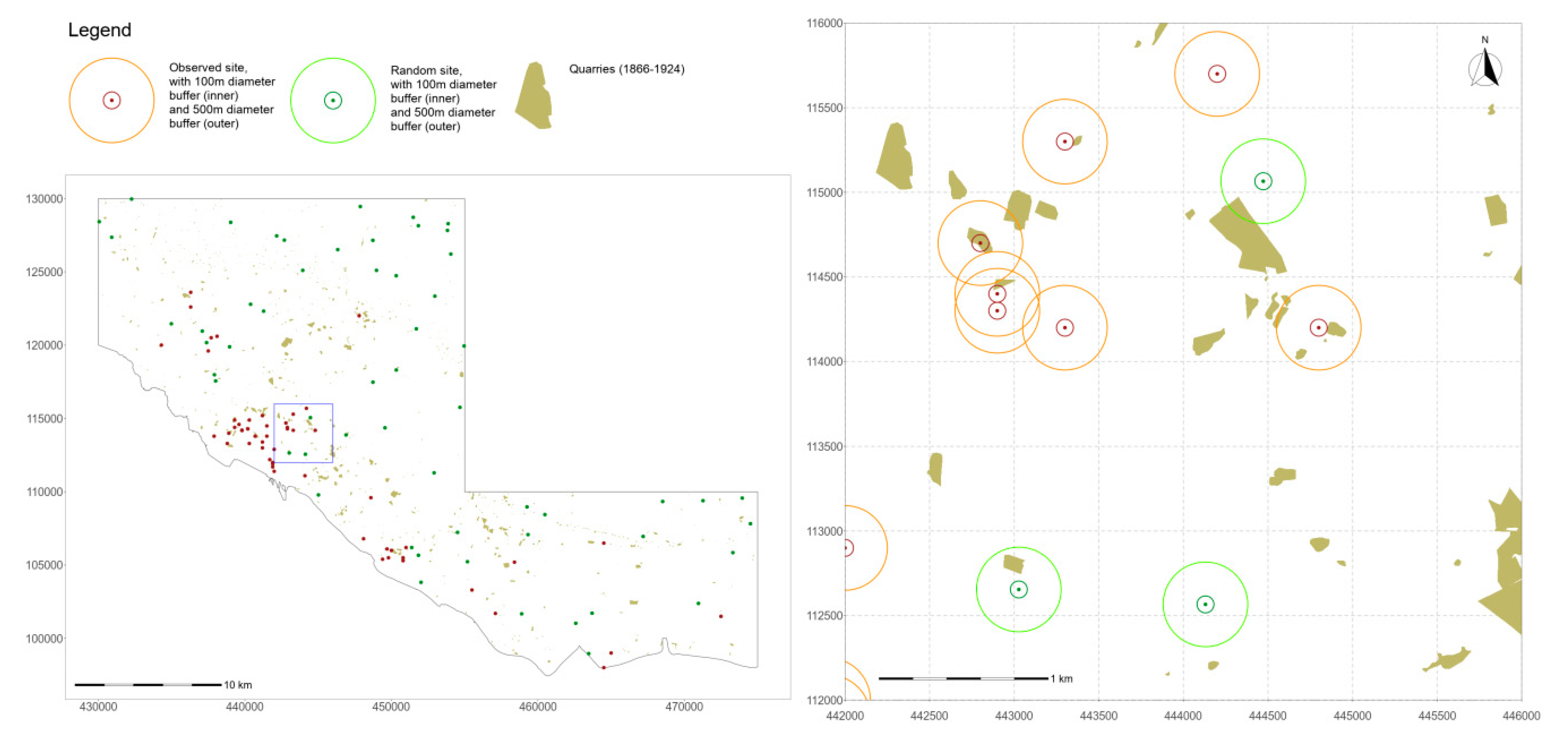
Thus, to account for this in the analysis, 100 m diameter buffers were generated around the Palaeolithic sites (Figure 2). Though this was done in R (Appendix A and B), it can also be easily be accomplished in any standard GIS software.

3.3.3. Random Sites Generation

Through the st_sample operation in the sf package [30], we generate the same number of random points as there are sites. The st_sample operation uses the uniform distribution (the generated pseudorandom values are uniformly, not normally, distributed), in line with the csr command from the splancs package [31] and standard reference texts on Monte Carlo simulation (e.g., [32]).To create our random sites with the same degree of uncertainty as our real sites, we add 100 m diameter buffers to the randomly generated points (Figure 2).

3.3.4. Overlay and Frequency Determination

The final part of the analysis involves overlaying the set of 100 m diameter buffers derived from the recorded sites onto the quarries layer and then counting the number of times the sites buffers intersect the quarries. The process is then repeated, but this time using a set of 100 m diameter buffers derived from the random sites generated as described above. To turn this procedure into a Monte Carlo simulation, it is now only necessary to build the random point generation procedure into a loop that simulates sites enough times for the appropriate statistical confidence level to be reached. In this case, we choose to run the analysis 100 times, equivalent to p = 0.01.

3.3.5. Script Programming

The above-described steps 3.3.1–3.3.4 were incorporated into two R Scripts which run successively and together comprise the MCSites tool. The tool, together with example data, can be accessed at https://drive.google.com/uc?export=download&id=1m-7KcIUCD-Zx3dQV_NCTBMGYT3Sr_mT4.
Copy and paste this link into the address bar of your browser and you will be able to download the “MCSites.zip” file. All that is needed to run the tool is the multi-platform software R, which can be installed from https://www.r-project.org/.
Once R is installed, the R software package sf will also need to be installed from the command line, as follows:
install.packages(“sf”)
If you copy and paste from this document, take care to replace the inverted commas with ones from your keyboard. The package tcltk is also needed, but is usually available as part of base R and does not need to be installed separately. Installed packages can be loaded with the command:
library(sf)
library(tcltk)
However, the necessary packages, once installed as described above, will be automatically loaded by the script file. To run the analysis from the script file provided at the line described above, open a new R window (or instance of RStudio), set the R working directory to the MCSites directory and execute the command “source (“scripts/main.R”)”.
setwd(“C:\\Users\\rh\\Documents\\MCSites”)##windows system
setwd(“/home/oct/MCSites”)##linux system
source(“scripts/main.R”)
The script will run giving a series of prompts to import the relevant data and carry out the Monte Carlo simulation. To execute the Monte Carlo analysis successfully, the user needs to do only what is described in this Section 3.3.5. More details are provided for advanced users or those interested in the process of code development in Appendix A.

4. Results

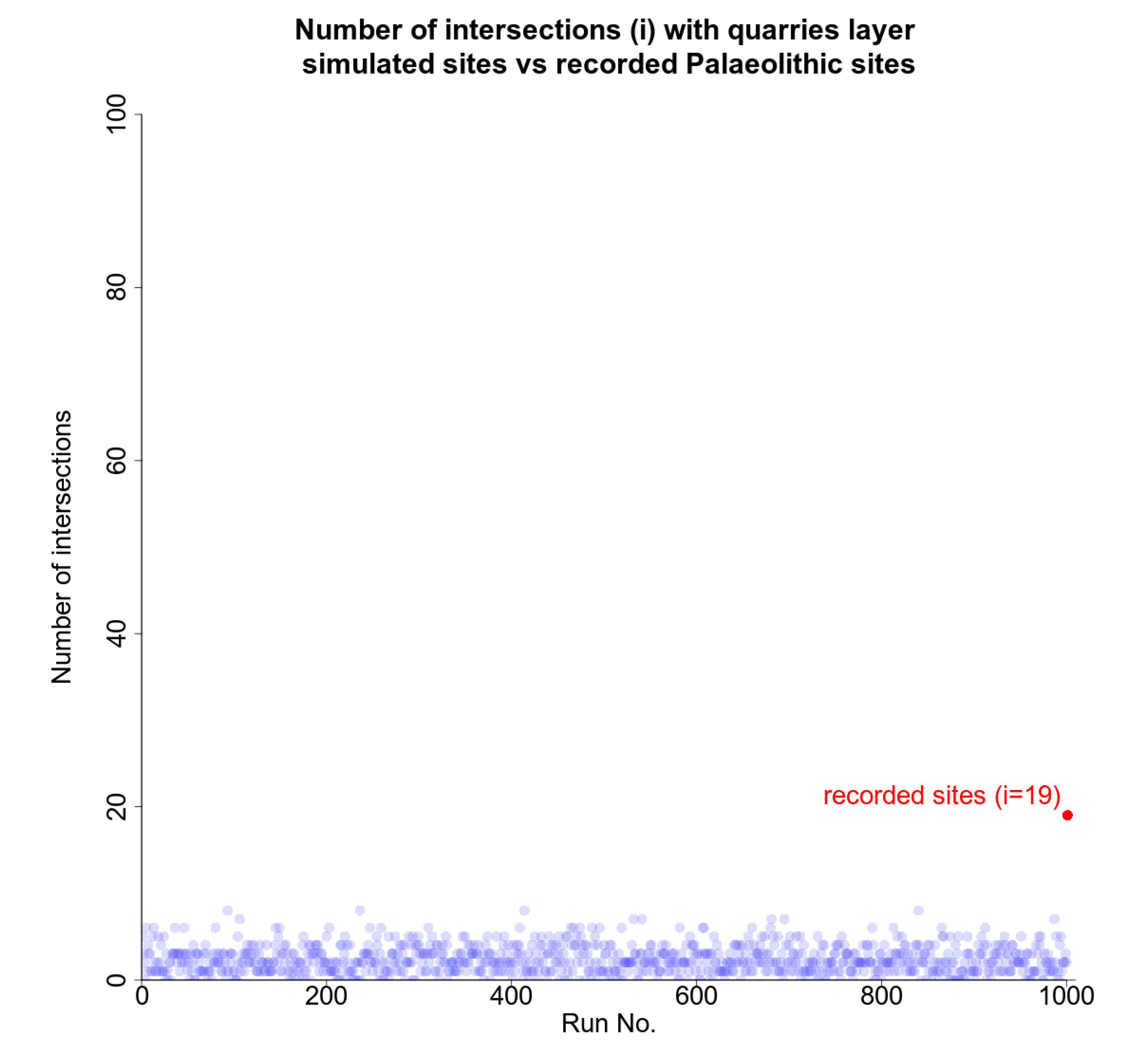
Given the level of uncertainty expected in the dataset (Section 3.3.2), the results are surprisingly unambiguous. Figure 3 shows clearly that the null hypothesis (Section 3.2) can be firmly rejected. For the 100-run test described in Section 3.3.4, the highest number of coincident random sites was 6, less than one third of the number of Palaeolithic sites that are coincident with the same map areas. On this basis, we can suggest with at least a 1% level of confidence (a result of this magnitude will not occur randomly more often than once in every 100 passes) that there is a significant association between Palaeolithic sites within the study area and quarries. To confirm this result, the test was repeated for 1000 runs on five separate occasions (Table 1). This had the effect of increasing the maximum number of hits in the random sites datasets to 8, but still did not approach the number of recorded sites coincident with the quarries layer. To show the effect on the test of the higher level of uncertainty in site location, the buffer diameter was increased from 100 to 200, and a further 3,1000 run tests were carried out (Table 1). Even allowing for a much-higher-than-expected uncertainty, the results still firmly suggest an association between recorded Palaeolithic sites and quarries.
While we cannot prove for certain that the location of the quarries is the cause of the spatial pattern (correlation is not causation), we show clearly that it is not likely to be independent from it. This offers a useful starting point for more in-depth examination of the individual sites, as well as offering a reminder that, for this ancient archaeological period, the location of archaeological finds is only very rarely an indicator of nearby hominin settlement activity.

5. Concluding Discussions

Though we have demonstrated our Monte Carlo testing approach with reference to quarries, the method is clearly applicable to any other kinds of landscape feature for which an association with archaeological sites could be postulated. This might include other archaeological features like ditches or boundaries (i.e. testing to see if finds are associated with them) and environmental variables like superficial geology, soil formations, or vegetation. It provides a bridge between somewhat antiquated aspatial techniques like the Χ2 test, which are difficult to successfully apply in a spatial context, and more developed analyses involving various kinds of regression. For testing association between archaeological sites and multiple explanatory variables, regression approaches are likely to be superior to this simple Monte Carlo test. However, the need to obtain and process suitable data, and the absence of obviously applicable explanatory variables for archaeological periods where climate, vegetation and landforms are all unrecognisably different from today, means that the Monte Carlo simulation approach described here is useful in a very wide variety of analysis contexts. For example, one very simple application, analogous to the case presented here, might be to investigate the association between cropland and archaeological sites detected by aerial photography, e.g., in the UK (e.g., [33]). As hot, dry years are known to provide ideal conditions for detection of archaeological sites from cropmarks on arable land, a clear association between arable land and archaeological sites might be expected. On the other hand, this would be expected to show some variation, depending on the type of crop and the type of site. A very strong association between sites and arable land might indicate a significant under-representation of archaeological sites on different land cover types, e.g., pasture, allowing different kinds of aerial remote sensing techniques (e.g., LIDAR) to be targeted to these areas.
The approach described also offers a way to account for spatial uncertainty in the form of imprecision in site location. Clearly, this is a less-than-perfect approximation because, in the absence of more precise coordinate information, the site must be represented as a probability zone rather than a single point, which makes it more likely that it will coincide with the selected features. However, if the same method is applied to the random points, they are also more likely to coincide with the selected features, and the two effects would be expected to cancel each other out. Despite the imperfect nature of the proposed solution, we feel that this approach is more honest than simply ignoring the issue. It is especially relevant for modern digital datasets which superimpose many objects recorded at differing scales and degrees of precision, like the point patterns produced by plotting HER records held by county archaeological offices in the UK. Finally, the approach described accounts only for spatial uncertainty. However, other kinds of uncertainty in archaeological data, such as temporal uncertainty, are also amenable to Monte Carlo approaches [34], and the development of a hybrid method that simultaneously addresses both spatial and temporal uncertainty would be an interesting direction for future work.
GIS approaches are widely used by archaeologists, and the R environment is an increasingly popular analysis tool. However, the GIS capability of R, recently enhanced with the addition of the simple features (sf) package [30], which we make use of in this analysis, remains under-appreciated. R is continually expanding and improving, and operations that were once convoluted or complex have become much easier over time. For example, Orton [35], describing the difficulty in finding software for point pattern analysis, lamented being unable to use the splancs package [36], because it required the purchase of S+, then an expensive proprietary statistics package. S+ has since been entirely integrated into R, and an early version of the Monte Carlo script described here made use of the splancs package. Mostly, the barrier to entry for archaeologists remains the perception that R is difficult to use (see, e.g., [37]). We hope to have dispelled this impression with the simple step-by-step “routemap” approach given here. For readers who wish to explore the analysis of archaeological point distributions in more detail, we recommend the spatstat package [38].
A final consideration, of key relevance to the topic of this Special Issue, is the high potential applicability of the proposed method as a rapid analysis tool for detection of association between archaeological surface or near-surface finds (e.g., recorded by an HER database or recovered from topsoil by metal detector survey or fieldwalking), and geophysical survey data. In its simplest form, as demonstrated here, the approach allows for very rapid comparison of a finds distribution against a map of geophysical anomalies. Clearly, if we are looking to identify an important archaeological feature, for example, the vicus associated with a Roman fort, being able to show association between particular finds and geophysical survey results is an important first step in any analysis. However, a more sophisticated application of the approach might seek to match scatters of finds of different dates with different geophysical plots corresponding to different techniques (ground-penetrating radar, magnetometer, etc.), or different depths.
Though we do not claim great sophistication (for more advanced applications of Monte Carlo simulation in archaeology, see, e.g., [16,21]), the approach we have demonstrated in this paper is statistically robust, free of the complexities associated with regression analysis, and simple to apply. This paper, therefore, hopes to serve as a starting point for development of more detailed studies incorporating Monte Carlo testing approaches for analysing patterns of association between archaeological sites and landscapes. Its potential seems particularly strong where landscapes are deeply buried or multiple uncertain interpretations exist, e.g., from palaeo-environmental reconstructions or results of geophysical surveys. We call for this approach to be more widely used in these contexts. The difficulties identified in the introduction to this article, especially around the potential of regional archaeological data to elucidate patterns of human activity in the landscape given the incompleteness of the archaeological record, deserve closer attention. Future work might usefully concentrate on the development of a toolbox of statistical approaches to address these issues more broadly.

Supplementary Materials

The MCSites tool, with example data required to run the Monte Carlo simulation, is available online at: https://drive.google.com/uc?export=download&id=1m-7KcIUCD-Zx3dQV_NCTBMGYT3Sr_mT4. All archaeological site data used in this paper are freely available from the archaeology data service at https://archaeologydataservice.ac.uk/archives/view/pashcc_eh_2007/downloads.cfm?volume=table&CFID=e6da3291-e098-4f25-83ff-c3c29ed9a555&CFTOKEN=0.

Author Contributions

Conceptualization, methodology, analysis and original draft preparation, R.J.H.; data collection and reviewing and editing, F.F.W.-S. and M.R.B. All authors have read and agreed to the published version of the manuscript.

Funding

The archaeological data used in this analysis were collected by the Palaeolithic Archaeology of the Sussex/Hampshire Coastal Corridor project, which ran between 2005 and 2007 and was funded by the Aggregates Levy Sustainability Fund (ALSF) as distributed by English Heritage (now Historic England). No funding was received for the research described in this paper, for the preparation of this manuscript for publication, or for the publication costs incurred.

Acknowledgments

The author(s) are grateful to COST Action SAGA: The Soil Science &Archaeo-Geophysics Alliance-CA17131 (www.saga-cost.eu), supported by COST (European Cooperation in Science and Technology), for the opportunity to participate in the Special Issue in which this paper appears.

Conflicts of Interest

The authors declare no conflict of interest. The funders had no role in the design of the study; in the collection, analyses, or interpretation of data; in the writing of the manuscript, or in the decision to publish the results.

Appendix A. Technical Description of the MCSites Tool

Appendix A.1. Data Import and Analysis Preparation in R
Geographical vector data, e.g., in shape file or geopackage format, can be imported into R in several ways. Here, we choose to do it with the sf package, as this package has recently been developed with the aim of unifying the GIS functionality provided across multiple packages and is now widely recommended as a replacement for earlier packages like maptools. The sample dataset provided with this paper (see additional data) is an ESRI shapefile of points expressed as xy coordinates under the UK Ordnance Survey national grid coordinate system (OSGB36). Points representing archaeological sites are imported as follows:
sites <- st_read(“data/example_sites.shp”)
plot(st_geometry(sites),pch = 18,col = “red”)
The same process is repeated for the study area, and for the features that the sites will overlap, the quarries are digitised from historic Ordnance Survey mapping.
study<- st_read (“data/esolent_studyarea.shp”)
feats<- st_read(“data/all_clipped_quarries.shp”)
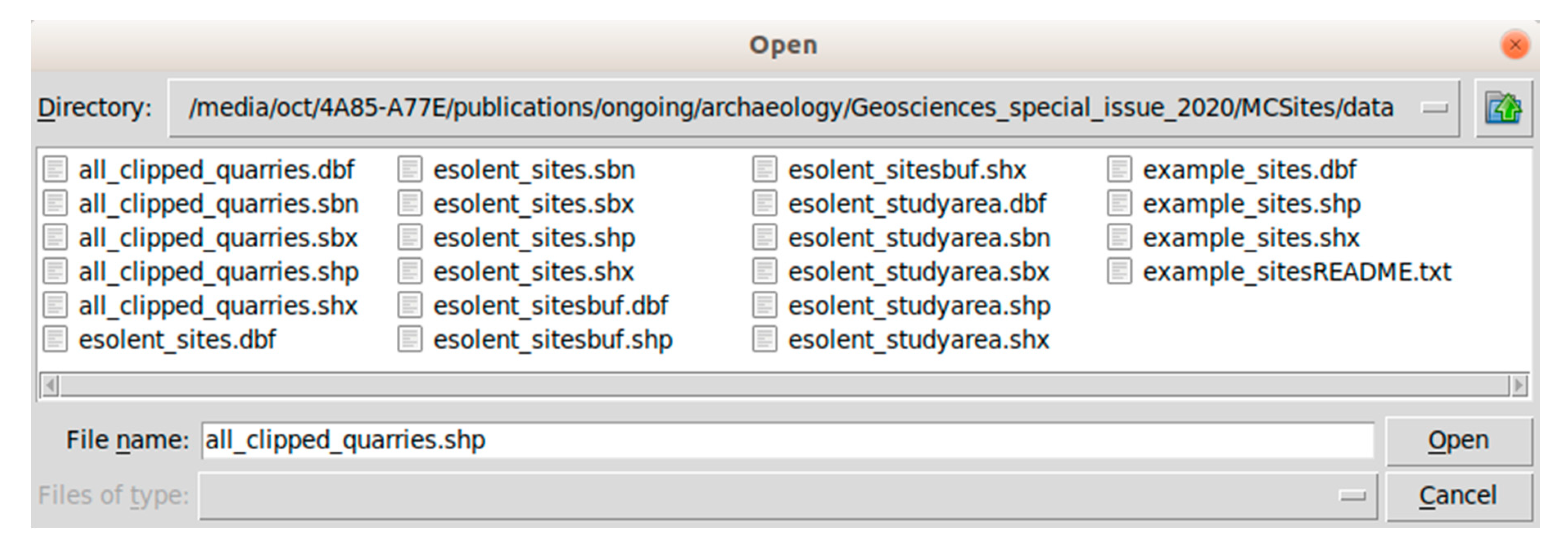
These operations are carried out through a series of dialogs (Figure A1) so the user does not need to execute the code by hand.
Figure A1. “Open” dialog, with shape file selected.
Geosciences 10 00326 g0a1
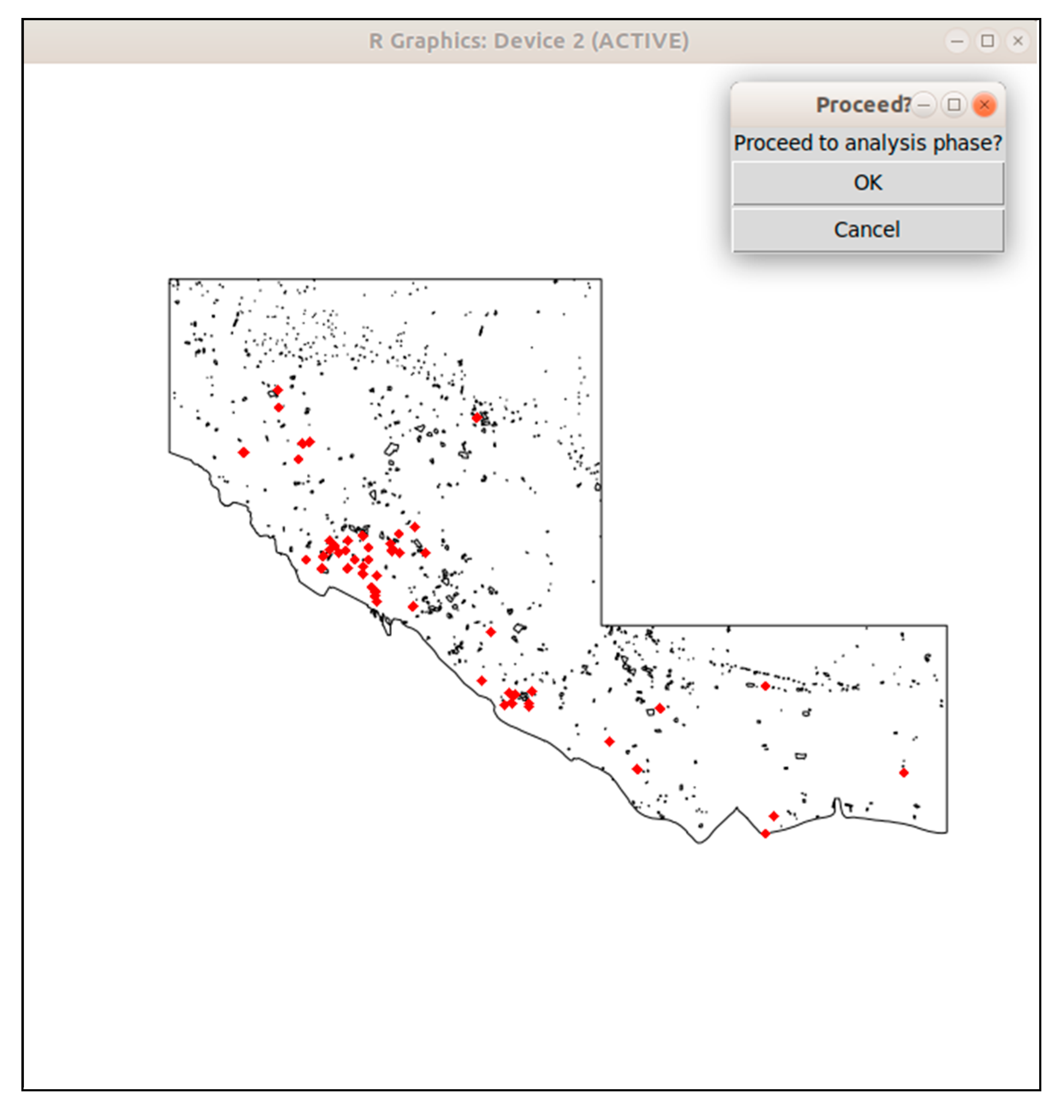
Once each of the three necessary layers (study area boundary, features to intersect with archaeological sites, archaeological sites) has been loaded, the “main.R” script file will plot each of the layers together, with sites shown in red, and prompt the user to continue. If the “OK” Option is selected, R will plot the selected layers (Figure A2) and proceed to the generation of random sites through the script file “rangen.R”. If the “Cancel” Option is selected, the dialog will close.
Figure A2. MCSites tool overlay maps and “Proceed” dialog.
Geosciences 10 00326 g0a2

Appendix A.2. Generation of Random Points Inside Study Area

Next, we generate the same number of random points as there are sites inside the study area boundary. This is accomplished using the st_sample command from the sf package, which applies a uniform sampling strategy as follows:
ranpoints<- st_sample((study$geometry),(length(sites$geometry)))
The random points generated are used in the script directly, but can be exported to a shape file if required:
st_write(ranpoints, “rpts.shp”, append = FALSE)

Appendix A.3. Buffering Sites and Random Points to Account for Uncertainty

To account for uncertainty (Section 3.3.2; Figure 2), the following procedure is followed:
uncert<- 100#uncertainty zone—the diameter of the circle equal to the size of the zone in which the site must fall
bufsize<- (as.numeric(uncert))/2#the buffer size is equal to the radius
sitesbuf<- st_buffer(sites, dist = bufsize) #buffer the real sites according to the specified uncertainty level
rptsbuf<- st_buffer(ranpoints, dist = bufsize) #buffer the random sites according to the specified uncertainty level

Appendix A.4. Overlay Features Layer with Sites and Random (Simulated) Sites

The st_intersects operation is applied as follows.
rg<- st_intersects(rptsbuf,feats)#intersects random sites and features
simoverlaps<- sum(lengths(rg) > 0) #gives number of overlaps for random sites and features
sg <- st_intersects(sitesbuf,feats) #intersects real sites and features
realoverlaps<- sum(lengths(sg) > 0) #gives number of overlaps for real sites and features

Appendix A.5. Run Monte Carlo Simulation

All that remains is to incorporate the above operations into a loop to run for as many times as the level of significance requires. For example, to test the hypothesis at a confidence level of p = 0.01, we would need to compare the number of overlaps between features and real sites with the number of overlaps between features and 100 separate sets of randomly generated sites. To generate a 100-run Monte Carlo simulation, the procedure would be as follows:
runs <- 100#input the required number of runs for the simulation
Then, generate a tabular data structure (in R known as a dataframe) to receive the results, with a number of rows equal to the number of runs:
dfmontecarlo = data.frame(matrix(vector(), as.numeric(runs), 2, dimnames = list(c(), c(“run_id”, “hits” ))), stringsAsFactors = F)#create an empty dataframe to receive the simulation results
dfreal = data.frame(matrix(vector(), 1, 2, dimnames = list(c(), c(“run_id”, “hits” ))), stringsAsFactors = F)#create an empty dataframe to receive the real results
Create a “for” loop that generates random points, buffers them, and overlaysthe features layer for the desired number of runs:
for (i in 1:as.numeric(runs)) {
ranpoints<- st_sample((study$geometry),(length(sites$geometry)))#generates as many random points as there are sites inside the boundary of the study area.
rptsbuf<- st_buffer(ranpoints, dist = bufsize) #buffer the random points according to the specified uncertainty level
rg<- st_intersects(rptsbuf,feats) #intersects random sites and features
simoverlaps<- sum(lengths(rg) > 0) #gives number of overlaps
dfmontecarlo[(i), 1] = i
dfmontecarlo[(i), 2] = simoverlaps
}
Overlay the real sites, and output the result to the dataframe:
sg <- st_intersects(sitesbuf,feats) #intersects real sites and features
realoverlaps<- sum(lengths(sg) > 0)#gives number of overlaps
dfreal[1,1] = i + 1
dfreal[1,2] = realoverlaps
tkmessageBox(message = “montecarlo simulation finished!”)
print(dfmontecarlo)
print(dfreal)
Optionally, we can join the two tables together and write the results out to a comma-separated file for easy opening in spreadsheet software:
dfboth<- rbind(dfmontecarlo,dfreal)#the last row will always be the real sites dataset
write.table(dfboth,”monte_carlo_test_results.csv”,sep =“,”,row.names = F)

Appendix B

MCSites tool, script 1 (main.R): This script uses the tcltk dialog environment to help the user import shape files to carry out the test.The user need only run this script, which calls the script “rangen.R” (Appendix B)
#####################################required libraries
require(sf)
require(tcltk)
#####################################script starts here
#the function to import the study area
filestudy<- function(){
tkmessageBox(message = “please choose study boundary (polygon.shp)”)
fileName<- tclvalue(tkgetOpenFile())
if (!nchar(fileName)) {
tkmessageBox(message = “No file was selected!”)
} else {
tkmessageBox(message = paste(“The file selected was”, fileName))
list(name = fileName)
}
}
#the function to import the features to be overlaid by sites
filefeat<- function(){
tkmessageBox(message = “please choose features for sites to intersect (polygon.shp)”)
fileName<- tclvalue(tkgetOpenFile())
if (!nchar(fileName)) {
tkmessageBox(message = “No file was selected!”)
} else {
tkmessageBox(message = paste(“The file selected was”, fileName))
list(name = fileName)
}
}
#the function to import the real sites
filesites<- function(){
tkmessageBox(message = “please choose sites (points.shp)”)
fileName<- tclvalue(tkgetOpenFile())
if (!nchar(fileName)) {
tkmessageBox(message = “No file was selected!”)
} else {
tkmessageBox(message = paste(“The file selected was”, fileName))
list(name = fileName)
}
}
#call the function to import the study area
con <- 0
N<- 3
while (con < 1) {
workfile<- filestudy()
filen<- toString(workfile$name)
filetype<- sapply(strsplit(filen, ““), function(filen, n) paste(tail(filen, n), collapse = ““), N)
if(filetype!= “shp”){
con <- 0
tkmessageBox(message = “shape file only (.shp) please”)
} else {
con <- 1
study <- st_read(filen)
}
}
#call the function to import the study area
con <- 0
N <- 3
while (con < 1) {
workfile<- filefeat()
filen<- toString(workfile$name)
filetype<- sapply(strsplit(filen, ““), function(filen, n) paste(tail(filen, n), collapse = ““), N)
if(filetype!= “shp”){
con <- 0
tkmessageBox(message = “shape file only (.shp) please”)
} else {
con <- 1
feats <- st_read(filen)
}
}
#call the function to import the study area
con <- 0
N <- 3
while (con < 1) {
workfile<- filesites()
filen<- toString(workfile$name)
filetype<- sapply(strsplit(filen, ““), function(filen, n) paste(tail(filen, n), collapse = ““), N)
if(filetype != “shp”){
con <- 0
tkmessageBox(message = “shape file only (.shp) please”)
} else {
con <- 1
sites <- st_read(filen)
}
}
plot(st_geometry(study))
plot(st_geometry(feats), add = TRUE)
plot(st_geometry(sites),pch = 18,col = “red”,add = TRUE)
tt<- tktoplevel()
tkwm.title(tt,”Proceed?”)
done <- tclVar(0)
# Create two buttons and for each one, set the value of the done variable to an appropriate value.
OK.but<- tkbutton(tt,text = “OK “,command = function() tclvalue(done) < −1)
Cancel.but<- tkbutton(tt,text = “Cancel”,command = function() tclvalue(done) < −2)
# Place the two buttons on the same row in their assigned window (tt).
tkgrid(tklabel(tt,text = “Proceed to analysis phase?”),sticky = “w”)
#tkgrid(tklabel(tt,text = “Proceed to analysis phase?”))
tkgrid(OK.but,sticky = “ew”)
tkgrid(Cancel.but,sticky = “ew”)
# Capture the event “Destroy” (e.g., Alt-F4 in Windows) and when this happens, assign 2 to done.
tkbind(tt,” < Destroy > “,function() tclvalue(done) < −2)
tkfocus(tt)
# Do not proceed with the following code until the variable done is non-zero.
#(But other processes can still run, i.e., the system is not frozen.)
tkwait.variable(done)
# The variable done is now non-zero, so we would like to record its value before
# destroying the window tt.If we destroy it first, then done will be set to 2
# because of our earlier binding, but we want to determine whether the user pressed
# OK (i.e., see whether done is equal to 1).
doneVal<- as.integer(tclvalue(done))
tkdestroy(tt)
if (doneVal == 1) {
#tkmessageBox(message = “will proceed to analysis phase”)
source(“rangen.R”)
} else if (doneVal == 2) {
#tkmessageBox(message = “exiting now!”)
}
#####################################script ends here.

Appendix C

MCSites tool, script 2 (rangen.R): This script is called automatically by the “main.R” script (Appendix B). It takes uncertainty input by the user in metres (e.g., 100), and creates buffers to represent this uncertainty for both random sites and real sites. It then runs a loop for a user-defined number of runs (e.g., 100), which generates a separate random-points dataset each time, and overlays it with the chosen feature layer. The overlaps between random sites and the features layer, and between real sites and the features layer are recorded in the dataframes (tables) dfmontecarlo and dfreal, respectively, which are then joined together and output to a .csv file.
#####################################required libraries
require(sf)
require(tcltk)
#####################################script starts here
tkmessageBox(message = “will now generate random numbers”)
uncert<- readline(“enter uncertainty (metres): “)
bufsize<- (as.numeric(uncert))/2
sitesbuf<- st_buffer(sites, dist = bufsize)
runs <- readline(“enter required number of runs: “)
#first generate a table with a number of rows equal to runs
dfmontecarlo = data.frame(matrix(vector(), as.numeric(runs), 2, dimnames = list(c(), c(“run_id”, “hits”))), stringsAsFactors = F)#create an empty dataframe to receive the simulation results
dfreal = data.frame(matrix(vector(), 1, 2, dimnames = list(c(), c(“run_id”, “hits”))), stringsAsFactors = F)#create an empty dataframe to receive the real results
for (i in 1:as.numeric(runs)) {
ranpoints<- st_sample((study$geometry),(length(sites$geometry)))#generates as many random points as there are sites inside the boundary of the study area.
rptsbuf<- st_buffer(ranpoints, dist = bufsize) #buffer the random points according to the specified uncertainty level
rg<- st_intersects(rptsbuf,feats) #intersects random sites and features
simoverlaps<- sum(lengths(rg) > 0)#gives number of overlaps
dfmontecarlo[(i), 1] = i
dfmontecarlo[(i), 2] = simoverlaps
}
sg <- st_intersects(sitesbuf,feats) #intersects real sites and features
realoverlaps<- sum(lengths(sg) > 0)#gives number of overlaps
dfreal[1,1] = i + 1
dfreal[1,2] = realoverlaps
tkmessageBox(message = “montecarlo simulation finished!”)
print(dfmontecarlo)
print(dfreal)
dfboth<- rbind(dfmontecarlo,dfreal)#the last row will always be the real sites dataset
write.table(dfboth,”monte_carlo_test_results.csv”,sep = “,”,row.names = F)
#To export random points to a shape file:
st_write(ranpoints, “rpts.shp”, append = FALSE)
#####################################script ends here

References

  1. Gaffney, V.; Stančič, Z. GIS Approaches to Regional Analysis: A Case Study of the Island of Hvar; University of Ljubljana, Research Institute of the Faculty of Arts & Science: Ljubljana, Slovenia, 1991. [Google Scholar]
  2. Holmes, K. GIS Simulation of the Earliest Hominid Colonisation of Eurasia; British Archaeological Reports: Oxford, UK, 2007; Volume 1597. [Google Scholar]
  3. Passmore, D.G.; Waddington, C.; Houghton, S.J. Geoarchaeology of the Milfield Basin, northern England; towards an integrated archaeological prospection, research and management framework. Archaeol. Prospect. 2002, 9, 71–91. [Google Scholar] [CrossRef]
  4. Deegan, A.; Foard, G. Mapping Ancient Landscapes in Northamptonshire; English Heritage; Liverpool University Press: Liverpool, UK, 2013. [Google Scholar]
  5. Carey, C.; Howard, A.J.; Knight, D.; Corcoran, J.; Heathcote, J. Deposit Modelling and Archaeology; University of Brighton: Brighton, UK, 2018. [Google Scholar]
  6. Bates, M.R.; Wenban-Smith, F.F. Palaeolithic Geoarchaeology: Palaeolandscape modelling and scales of investigation. Landscapes 2011, 12, 69–96. [Google Scholar] [CrossRef]
  7. Bates, M.R.; Stafford, E. Thames Holocene: A geoarchaeological Approach to the Investigation of the River Floodplain for High Speed 1, 1994–2004; Wessex Archaeology: Salisbury, UK, 2013; p. 280. [Google Scholar]
  8. R Core Team. R: A Language and Environment for Statistical Computing; R Foundation for Statistical Computing: Vienna, Austria, 2020. [Google Scholar]
  9. Hodder, I.; Orton, C. Spatial analysis in Archaeology. 1976. Available online: https://www.bcin.ca/bcin/detail.app?id=51540 (accessed on 18 August 2020).
  10. Wheatley, D.; Gillings, M. Spatial Technology and Archaeology: The Archaeological Applications of GIS; CRC Press: Boca Raton, FL, USA, 2002. [Google Scholar]
  11. Berry, K.J.; Kvamme, K.L.; Mielke, P.W., Jr. Improvements in the permutation test for the spatial analysis of the distribution of artifacts into classes. Am. Antiq. 1983, 48, 547–553. [Google Scholar] [CrossRef]
  12. Orton, C.R. Stochastic process and archaeological mechanism in spatial analysis. J. Archaeol. Sci. 1982, 9, 1–23. [Google Scholar] [CrossRef]
  13. Johnson, I. Local Density Analysis: A New Method for Quantitative Spatial Analysis. In Computer Applications in Archaeology; University of Birmingham: Birmingham, UK, 1977; pp. 90–98. Available online: https://proceedings.caaconference.org/paper/10_johnson_caa_1977/ (accessed on 18 August 2020).
  14. Barceló, J.A. Archaeological Thinking: Between space and time. Archeol. Calc. 2002, 13, 237–257. [Google Scholar]
  15. Fisher, P.; Farrelly, C.; Maddocks, A.; Ruggles, C. Spatial analysis of visible areas from the Bronze Age cairns of Mull. J. Archaeol. Sci. 1997, 24, 581–592. [Google Scholar] [CrossRef]
  16. Crema, E.R.; Bevan, A.; Lake, M.W. A probabilistic framework for assessing spatio-temporal point patterns in the archaeological record. J. Archaeol. Sci. 2010, 37, 1118–1130. [Google Scholar] [CrossRef] [Green Version]
  17. Metropolis, N.; Ulam, S. The montecarlo method. J. Am. Stat. Assoc. 1949, 44, 335–341. [Google Scholar] [CrossRef] [PubMed]
  18. Ulam, S. Random processes and transformations. In Proceedings of the International Congress on Mathematics, Cambridge, MA, USA, 30 August–6 September 1952; Volume 2, pp. 264–275. [Google Scholar]
  19. Shortridge, A.M.; Goodchild, M.F. Geometric probability and GIS: Some applications for the statistics of intersections. Int. J. Geogr. Inf. Sci. 2002, 16, 227–243. [Google Scholar] [CrossRef]
  20. Lake, M.W.; Woodman, P.E. Visibility studies in archaeology: A review and case study. Environ. Plan. B Plan. Des. 2003, 30, 689–707. [Google Scholar] [CrossRef] [Green Version]
  21. Bevan, A.; Crema, E.; Li, X.; Palmisano, A. Intensities, interactions and uncertainties: Some new approaches to archaeological distributions. In Computational Approaches to Archaeological Spaces; Bevan, A., Lake, M., Eds.; Left Coast Press: Walnut Creek, CA, USA, 2013; pp. 27–52. [Google Scholar]
  22. Baddeley, A.; Diggle, P.J.; Hardegen, A.; Lawrence, T.; Milne, R.K.; Nair, G. On tests of spatial pattern based on simulation envelopes. Ecol. Monogr. 2014, 84, 477–489. [Google Scholar] [CrossRef] [Green Version]
  23. Bates, M.R.; Wenban-Smith, F.; Briant, R.; Bates, C.R. 2007: Curation of the Sussex/Hampshire Coastal Corridor Lower/Middle Palaeolithic Record. Final Report. English Heritage/Archaeology Data Service. Available online: https://archaeologydataservice.ac.uk/archives/view/pashcc_eh_2007/overview.cfm?&CFID=7128b977-af16-46f1-8ea7-13dff21fc4d6&CFTOKEN=0#dig1 (accessed on 18 August 2020).
  24. Evans, J. Ancient Stone Implements, Weapons and Ornaments of Great Britain; Longmans, Green, Reader and Dyer: London, UK, 1872. [Google Scholar]
  25. Bates, M.; Wenban-Smith, F.; Briant, R.; Marshall, G. Palaeolithic Archaeology of the Sussex/Hampshire Coastal Corridor; Unpublished EH/ASLF Final Report; 2004. [Google Scholar]
  26. MacRae, R.J. New Lower Palaeolithic finds from gravel pits in central southern England. Lithics J. Lithic Stud. Soc. 1991, 12. Available online: https://www.semanticscholar.org/paper/New-lower-Palaeolithic-Finds-from-Gravel-Pits-in-Macrae/fd84217ab9ad11fa86004106b015fda7b39d1d57 (accessed on 18 August 2020).
  27. Hosfield, R. The Palaeolithic of the Hampshire Basin: A Regional Model of Hominid Behaviour during the Middle Pleistocene; BAR British Series 286; Archaeopress: Oxford, UK, 1999. [Google Scholar]
  28. Hatch, M.; Davis, R.J.; Lewis, S.G.; Ashton, N.; Briant, R.M.; Lukas, S. The stratigraphy and chronology of the fluvial sediments at Warsash, UK: Implications for the Palaeolithic archaeology of the River Test. Proc. Geol. Assoc. 2017, 128, 198–221. [Google Scholar] [CrossRef]
  29. Hewitt, R.J. The Lower and Middle Palaeolithic Archaeology of the Eastern Solent. Unpublished MLitt Dissertation, University of Newcastle-upon-Tyne, Newcastle-upon-Tyne, UK, 2005. Available online: https://www.researchgate.net/profile/Richard_Hewitt3/publication/325116224_The_Lower_and_Middle_Palaeolithic_Archaeology_of_the_Eastern_Solent_a_map-based_investigation_using_GIS/links/5af8b0d80f7e9b026bec6dde/The-Lower-and-Middle-Palaeolithic-Archaeology-of-the-Eastern-Solent-a-map-based-investigation-using-GIS.pdf (accessed on 18 August 2018).
  30. Pebesma, E. sf: Simple Features for R; R package version 0.9–4; 2020. Available online: https://r-spatial.github.io/sf/articles/sf1.html (accessed on 18 August 2020).
  31. Bivand, R.; Rowlingson, B.; Diggle, P.; Petris, G.; Eglen, S. Package “Splancs”, R documentation. Available online: https://cran.r-project.org/web/packages/splancs/splancs.pdf (accessed on 18 August 2020).
  32. Robert, C.; Casella, G. Monte Carlo Statistical Methods; Springer Science & Business Media: Berlin/Heidelberg, Germany, 2013. [Google Scholar]
  33. Bewley, R.H. Aerial survey for archaeology. Photogramm. Rec. 2003, 18, 273–292. [Google Scholar] [CrossRef] [Green Version]
  34. Crema, E.R. Modelling temporal uncertainty in archaeological analysis. J. Archaeol. Method Theory 2012, 19, 440–461. [Google Scholar] [CrossRef]
  35. Orton, C. Point pattern analysis revisited. Archeol. Calc. 2004, 15, 299–315. [Google Scholar]
  36. Rowlingson, B. and Diggle, P. 1993 Splancs: Spatial point pattern analysis code in S-Plus. Comput. Geosci. 1993, 19, 627–655. [Google Scholar] [CrossRef]
  37. Baxter, M.J. Notes on Quantitative Archaeology and R; Nottingham Trent University: Nottingham, UK, 2015. [Google Scholar]
  38. Baddeley, A.J.; Turner, R. Spatstat: An R Package for Analyzing Spatial Point Patterns. J. Stat. Softw. 2005, 12, 6. [Google Scholar] [CrossRef] [Green Version]
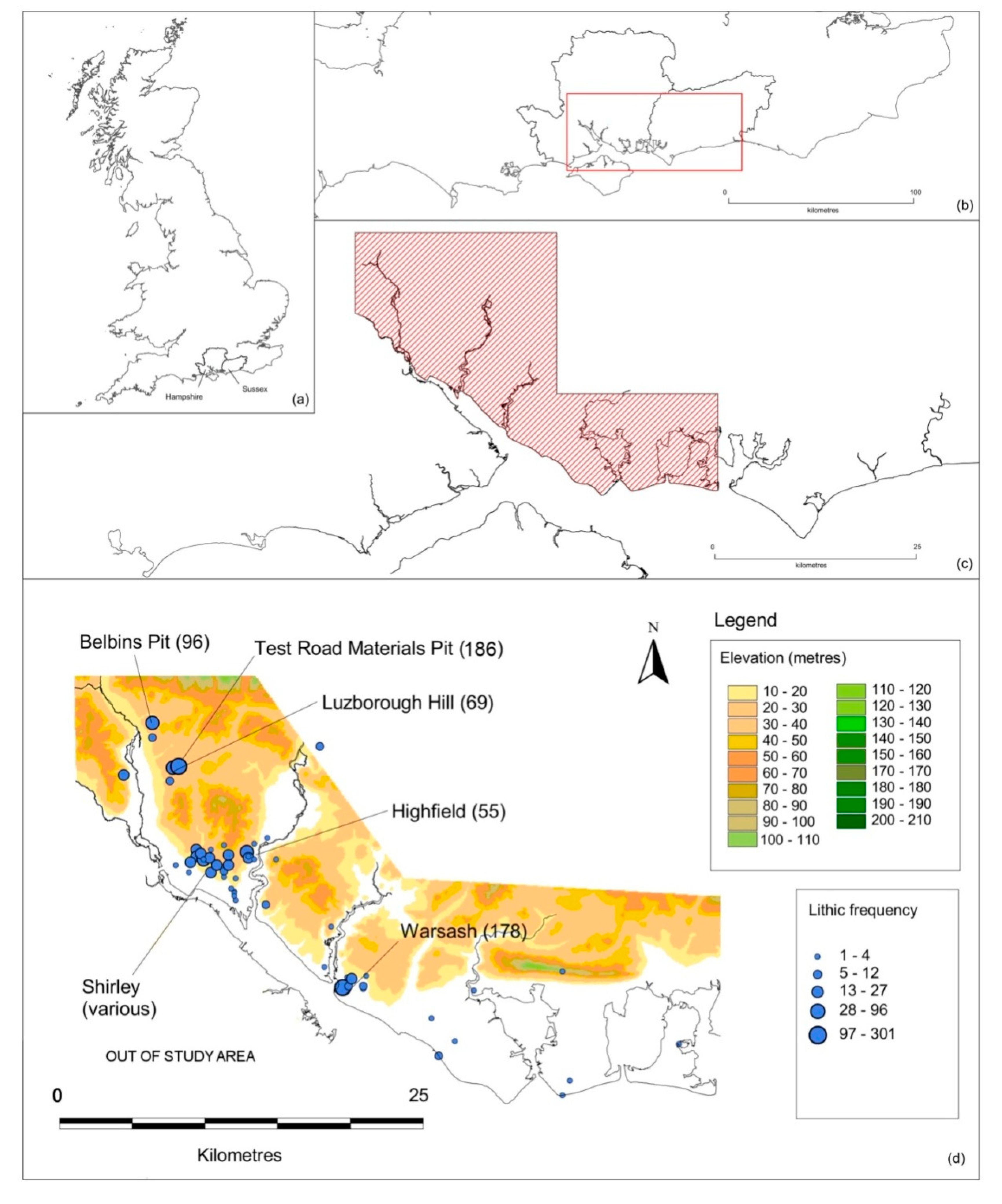
Figure 1. (a) Hampshire and Sussex in Southern England; (b) the Sussex/Hampshire coastal corridor catchment area; (c) Eastern Solent-focussed study area; (d) Palaeolithic sites of the study area, showing modern-day elevation above sea level, mapped by frequency of lithics discovered at each site. Highest lithic yield sites are named, with lithic counts following in parentheses.
Geosciences 10 00326 g001
Figure 2. Observed sites, random sites and uncertainty buffers. Inner (100 m diameter) buffers were used in this analysis. The greater the uncertainty, the larger the buffer, and hence, the higher the probability of intersection between sites and quarries.
Geosciences 10 00326 g002
Figure 3. No. of recorded Palaeolithic sites (total n = 57) intersecting with quarries, versus number of random sites (total n = 57) intersecting with quarries, for 1000 Monte Carlo simulation runs (Run No. 1 in Table 1, below). Test No. 1001 is the 57 recorded Palaeolithic sites. Site/quarries intersection counts for Monte Carlo simulation shown in blue, recorded sites in red.
Geosciences 10 00326 g003
Table 1. Monte Carlo Simulation test results for 8 simulation passes of 1000 runs. Note how increasing the size of the uncertainty buffer increases the number of hits for both recorded sites and randomly simulated sites.
Run NumberNumber of SimulationsMean FrequencyMedianModeMinMaxRecorded SitesUncertainty (m)
110002.323220819100
210002.206220819100
310002.233220819100
410002.304220819100
510002.243210819100
610004.3714401522200
710004.274401222200
810004.284401522200