Understanding Wetlands Stratigraphy: Geophysics and Soil Parameters for Investigating Ancient Basin Development at Lake Duvensee

Abstract

We present a case study of a bog showing how an integrated approach of multi-method geophysical sounding and local soil sampling can be used to identify, differentiate, and map organic sediments. Our study is based on ground-penetrating radar (GPR), electrical resistivity tomography (ERT) and shear-wave seismic (SH seismic) profiling applied to sediments of the former Lake Duvensee (northern Germany), nowadays a bog. This is a well-known locality for remains from the Mesolithic hunter-gatherers’ occupation that has been attracting archaeological and geoarchaeological research for100 years. The bog is embedded in low conductive glacial sand and is characterized by layers of different gyttja sediments (detritus and calcareous). The present study was conducted in order to identify the bog morphology and the thickness of the peat body and lake sediments, in order to understand the basin evolution. To validate the geophysical results, derived from surface measurements, drilling, soil analyses as well as borehole guided wave analysis of electromagnetic waves and Direct-Push (DP-EC) have been carried out and used for comparison. It turned out that each method can distinguish between sediments that differ in grain size, particularly between peat, lake sediments (gyttjas and mud) and basal glacial sand deposits. GPR is even able to separate between strongly and weakly decomposed peat layers, which is also clear considering resistivity variations in the ERT computation. From the association between geophysical properties and sediment analysis (e.g., water content and organic matter) different gyttjas were distinguished (coarse and fine) and seismic velocity was correlated to bulk density. Moreover, GPR and SH-wave seismics present different resolutions, confirming that the latter allows measurements, which are more focused on determining the extension of basal sand deposits, the depth of which is difficult to reach with GPR. Representative values of electrical resistivity, dielectric permittivity, and shear wave velocity have been determined for each sediment type and are therefore available to complete the investigation of wetland environments. Fine grained lake sediments were difficult to differentiate by the applied methods. This could be a result of high ionic concentration within the permanent groundwater body, partly masking the sediment properties.

1. Introduction

From prehistoric to historic times, floodplain margins, lake shorelines and coasts have been preferential settlement areas. Sites with water access provided favourable conditions for human activity and habitats [1,2,3]. Therefore, wetland margins are important zones in archaeological and geoarchaeological research [4,5], despite the often difficult exploration conditions, e.g., water logging or the groundwater impact [6]. The palaeoenvironmental reconstruction of wetland development depends critically on knowledge of the peatland stratigraphy, including the thickness and distribution of the peat deposit, within-peat layering, and the underlying lake sediments (gyttjas).

Peat forms through the accumulation of partially decomposed plant biomass in fens, bogs, and swamps [7]. The physical properties of any sediment are dependent to a large degree on porosity and pore-size distribution, which in turn are related to particle-size distribution. In peat, particle size and structure and the resulting porosity are controlled primarily by the degree of decomposition. Undecomposed peats contain many large pores, highly irregular and interconnected, that permit water movements. Highly decomposed peat contains smaller open pores, and also those pores that are closed or partially closed [8,9]. Peat is thus a dual-porosity medium that includes a ‘mobile region’ through which water moves relatively easily, and an ‘immobile region’ with negligible fluid flow velocity [10]. It is also a sedentary deposit, which means that the degree of decomposition generally increases with depth below the ground surface, while the geometric mean pore diameter and active porosity simultaneously decrease [10,11]. Peat is a highly compressible material [12], and this property is also controlled by the structure and arrangement of its pores [13], factors that are largely controlled by the degree of decomposition [12]. Decomposed peat at greater depths typically shows lower active porosity and compressibility. Within the peat deposits, the degree of decomposition has an influence, too, organic matter content decreases and bulk density increases with the degree of decomposition [14].

Gyttja sediments are layers with varying organic matter content that developed in low-energy subaqueous environments. The term ‘gyttja’ was introduced by [15] as a combination of organic and inorganic materials precipitated from a lake water column via biogeochemical processes. Organic matter that originates from aquatic life within the lake and input from the lake catchment accumulates at the sediment–water interface when its specific weight exceeds that of water. In a fresh state, gyttjas are very soft and hydrous. Organic gyttja often shows a dark greenish-gray to black color depending on the organic matter content. Calcareous gyttja is of rather a yellowish to pink color. Detritus gyttja appears similar to decomposed peat because it contains plant remains, still encased in a predominantly fine and rather elastic matrix; the fine lake sediments appear instead to have similar physical properties like clay deposits (e.g., grain size of silt and clay, and high ionic concentration of the pore water, which creates high conductivities such as those of clay minerals) [16].Depending on the sedimentary environment, gyttjas can vary in their organic matter content and may thus be predominantly mineral or organic deposits [17,18]. The proportion of mineral and organic matter contents influences the mechanical and hydrological properties of gyttja sediments [19].

Geoarchaeological investigations of peatland stratigraphy require integrated multidisciplinary approaches on varying scales, including surveys and geophysical prospecting, as well as medium-, small- and micro-scale drilling campaigns and excavations, to ground truth the results [20,21,22]. Drilling provides detailed information about the vertical stratigraphy, but usually with a low spatial resolution due to the time-consuming character of this method. Additionally, inter-drilling point sections have to be interpolated, resulting in an unknown uncertainty about small-scale changes in the stratigraphy. This disadvantage can be improved by combining drilling with non-invasive geophysical methods, ground-penetrating radar (GPR), electrical resistivity tomography (ERT) and S-wave seismics, which allow a laterally continuous mapping of the lithological change [23,24].

Numerous studies have been carried out in different bogs and peatlands showing the potential of wetland geophysics. However, there is still some scepticism about the usefulness of this discipline [25] with regard to the variability of exploration conditions. Ground-penetrating radar (GPR) has been widely used to analyze peat deposits due the low electrical conductivity of the peat [20,26,27,28,29,30,31], which allows for a large penetration depth. Moreover, the change in water content with respect to the mineral sediment provides strong reflections for excellent geophysical imaging [32]. Several studies [33,34,35] give tables of dielectric permittivity for a range of sediment types and other materials (summarized here in Appendix A). They show that the permittivity values have large ranges, especially for wetland sediments. The authors of [25] review the outcome of different case studies in wetland sediments, showing that dielectric permittivity can be highly variable if not waterlogged. The boundary between the peat and the underlying mineral sediment is identifiable because of the sharp reduction in the volumetric water content between the peat and the mineral soil below (e.g., [11,16,28,36]). GPR profiles within peat often showed patterns of reflections [27] and suggested that these reflections strongly match variations in peat moisture content. The authors of [11,26,28] could thus identify the boundary between uppermost poorly decomposed peat (“acrotelm”) and underlying well-decomposed peat (“catotelm”).

The success of detecting such interfaces depends on the dielectric contrast between the different layers and is thus site-specific. The same is observed if we consider the interfaces between peat and gyttja layers. The authors of [16], for instance, illustrated a distinction between peat and organic gyttja layer, whereas [37] could not. Gyttja deposits show variable bulk density depending on their organic matter content [38], thus the dielectric properties broadly differ too. Therefore, gyttja was often not further differentiated and it is difficult to decide whether different gyttja layers were detected or not [18].The electrical conductivity depends linearly on the concentration of total dissolved solids in the peat pore waters. The authors of [27] found that the ionic concentration, and thus the electrical conductivity, increases linearly from the surface to basement for peat deposits. High fluid electrical conductivity in peat, or a high percentage of clayish sediments in the mineral soil, can excessively attenuate radar wave propagation, reducing the depth of penetration in peat and usually prevent recording of reflections from below the mineral soil contact underlying peat bogs [20,27].

Geoelectric measurements are less common in wetlands but have become an important tool for geoarchaeology. Electrical conductivity is the inverse of electrical resistivity and former studies have demonstrated that peat is chargeable, attributed to the high surface-charge density of partially decomposed organic matter [28,39].The electric conductivity depends strongly on temperature, which differs seasonally, and on whether samples are measured in the field or in the laboratory [27,40]. ERT can assist peatland studies as it can provide stratigraphic information from beneath the mineral soil contact [27,28]. However, little is known so far about the relationship between electrical conductivity and peat properties under different site conditions. The authors of [16,18,41] found that the total amount of solutes in the pore fluid and the cation exchange capacity are the properties that determine electrical conductivity of poorly decomposed Sphagnum peat. Moreover, the authors claim that water content and cation exchange capacity are mainly correlated with electrical conductivity.

The application of seismics for geoarchaeological research is not widespread but has lately been intensified due to exemplary results [23,42,43,44,45,46,47,48]. SH-wave seismics are directly sensitive to the rigidity of soil layers and are capable of resolving stratigraphic interfaces at much larger depths than GPR [42,49]. SH-wave sounding can identify and differentiate soft soils such as fine-grained lake sediments or swampy organic deposits [23], which are characterized by slow seismic velocities.

We present a multi-method geophysical survey at the Duvensee palaeolake in south eastern Schleswig-Holstein, northern Germany, which is well known for Early Mesolithic hunter-gatherer archaeology on the Northern European Plain [50].

Our study has three major objectives:

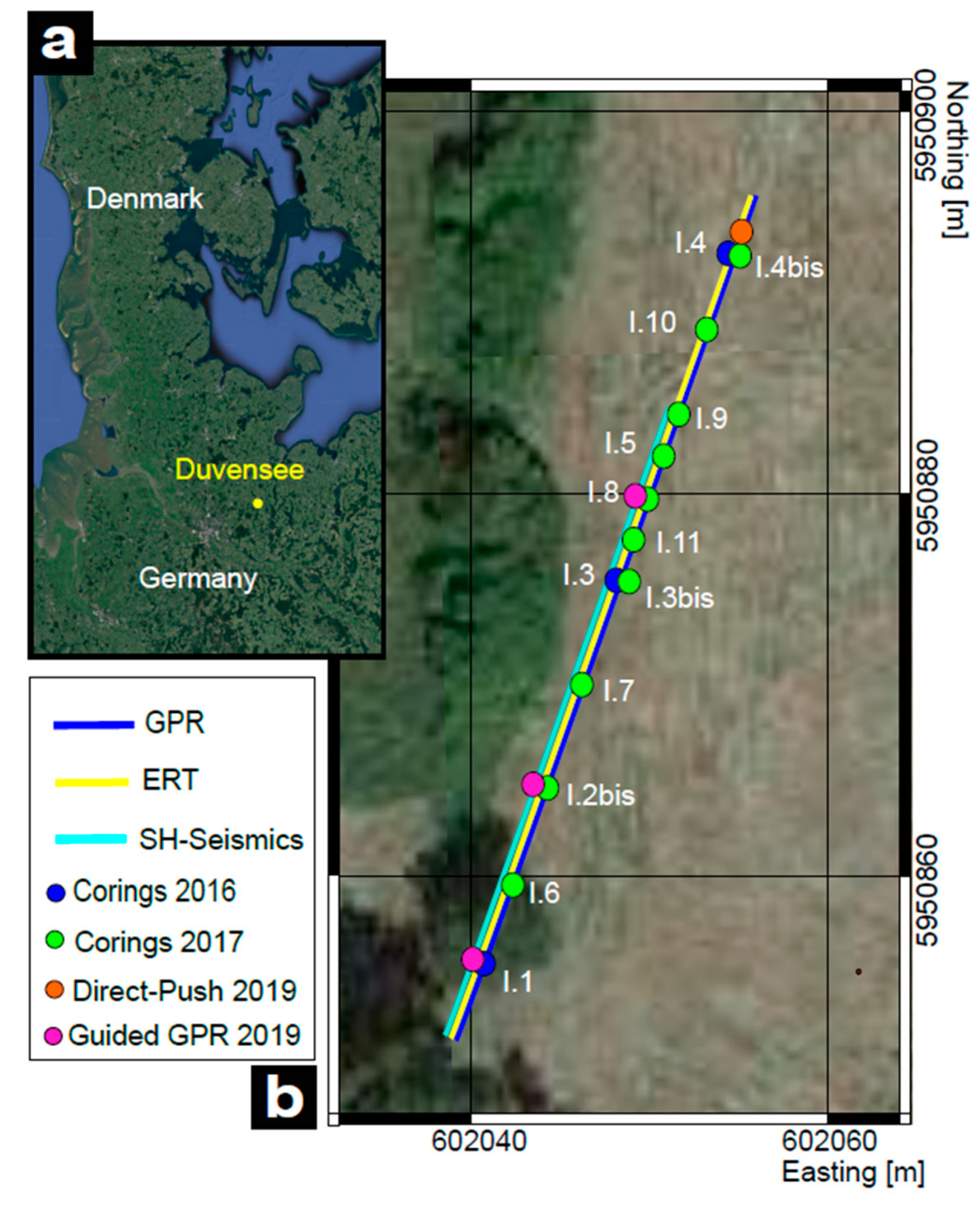
• To identify and continuously map the main stratigraphic units that fill the ancient Lake Duvensee to facilitate an understanding of the basin evolution. For this purpose, we combined sampling by drilling with ground-penetrating radar (GPR), electric resistivity tomography (ERT), and seismic sounding with shear waves (SH-waves seismic).
• To evaluate the suitability of GPR, ERT and SH-wave seismic to detect peat properties, paying attention to the identification of different gyttja layers.
• To determine the conditions under which peat and gyttja layers can be identified and distinguished in terms of geophysical parameters, particularly resistivity, shear wave velocity and dielectric permittivity.

The geophysical results are presented for each method and compared with the stratigraphy from the drilling to ground truth measurements. Moreover, sediment properties (i.e., degree of decomposition, water content, ion concentration) of the main sediment types (peat, gyttja, silty clay and sand) are discussed together with electrical resistivity, SH-wave velocities and electromagnetic wave velocity variations, to validate the geophysical results. The presented geophysical surveys contribute to understanding wetland archaeology focusing on how to combine methods to get more information on the stratigraphy. Moreover, the possibility of separating strongly from weakly degraded peat would be extremely helpful for the archaeological research to evaluate the preservation conditions of archaeologically relevant layers, which might direct further investigations. Only few of previous surveys of wetlands employed more than one technique to the same area, making it hard to comparatively evaluate the results produced. Our case study shows the benefits of using multiple techniques, and the key role ground-truthing plays.

2. Area of Investigation and Landscape Development

The ancient Lake Duvensee in Schleswig-Holstein (northern Germany) is one of the prime locations in northern Europe for early Holocene archaeological research. The ancient lakebed was formed during the older Dryas as a dead-ice hole left by the retreating Fennoscandian ice sheet [51]. Past stratigraphic investigations revealed a complex basin topography, characterized by numerous deeps and sand banks [52], which were used by Early Mesolithic hunter-gatherer groups to establish temporary camps. The gradual infilling of the basin led to the disappearance of the former lake, and, by the 19th century CE, most of the basin was occupied by a bog.

The sediment succession near the shorelines generally exhibits a gradual shallowing of the depositional environment. The majority of the deposits are typical lake sediments, such as calcareous gyttja, algal gyttja and coarse detrital gyttja. The sediment cores have shown that, in spite of similar depositional conditions, strong lateral variations in sediment facies are present. The complicated alterations observed in the drilling attest to multiple changes in lake level [52]. This area has been the subject of archaeological research for almost 100 years, showing the presence of 23 different locations of Early Mesolithic hunter-gatherer groups and Neolithic farmers. Based on GPR sounding, [31] developed a 3D model of the Duvensse bog and its stratigraphy, including five islands, which emerged from the retreating water over time, making them suitable for Mesolithic camps. These results confirmed and complemented previous archaeological surveys [53]. The estimated emergence times of the mapped islands agree with the spatio-temporal pattern of the previous archaeological finds [53].

Coherent overviews of the research at ancient Lake Duvensee have been given by [50,53,54]. The area has also been the subject of different geophysical campaigns aimed at improving the knowledge regarding the evolution of the basin. After a large-scale GPR survey carried out in November 2016, more detailed geophysical measurements have been conducted focusing on a small scale. For ground truthing the stratigraphy of the basin, a reference profile has been chosen, and different geophysical measurements have been applied between 2018 and 2019 (Figure 1, see also [31]). Work at Duvensee, particulalry the results of GPR and coring surveys, has been described in detail in [31], and is only briefly summarized here (see Section 4.2).

3. Methodology

3.1. Ground-Penetrating Radar (GPR)

3.1.1. GPR Surface Profiling

The GPR system consists of a transmitting and a receiving antenna. The former emits an electrmagnetic wave and the latter detects the transmitted wave, which is partially reflected in the subsurface at interfaces [33]. The propagation of a radar signal depends on the dielectric permittivity (ε_r), which controls the propagation velocity and reflection strengths, and the electrical conductivity (σ), which mainly influences the signal attenuation. The signal strength and center frequency of radar signals decrease during wave propagation due to energy absorption (e.g., [55]). High water content and clayish-loamy sediments, for instance, strongly attenuate the radar signal and reduce the depth of investigation [33].

A GSSI GPR Antenna with 200 MHz frequency was used to perform common offset data acquisition in the Duvensee area. The presented profile (50 m long, blue line in Figure 1) is part of a survey made in November 2016. The measurement details and the processing steps are described in [31]. The reflections associated with the main layers visible in the cores (basal sands, fine minerogenic sediments, fine and coarse organic deposits) have been recognized and picked using the Kingdom IHS Software. The conversion from time to depth was made using the corresponding velocity values derived from CMP (common-midpoint) measurements (see [31]).

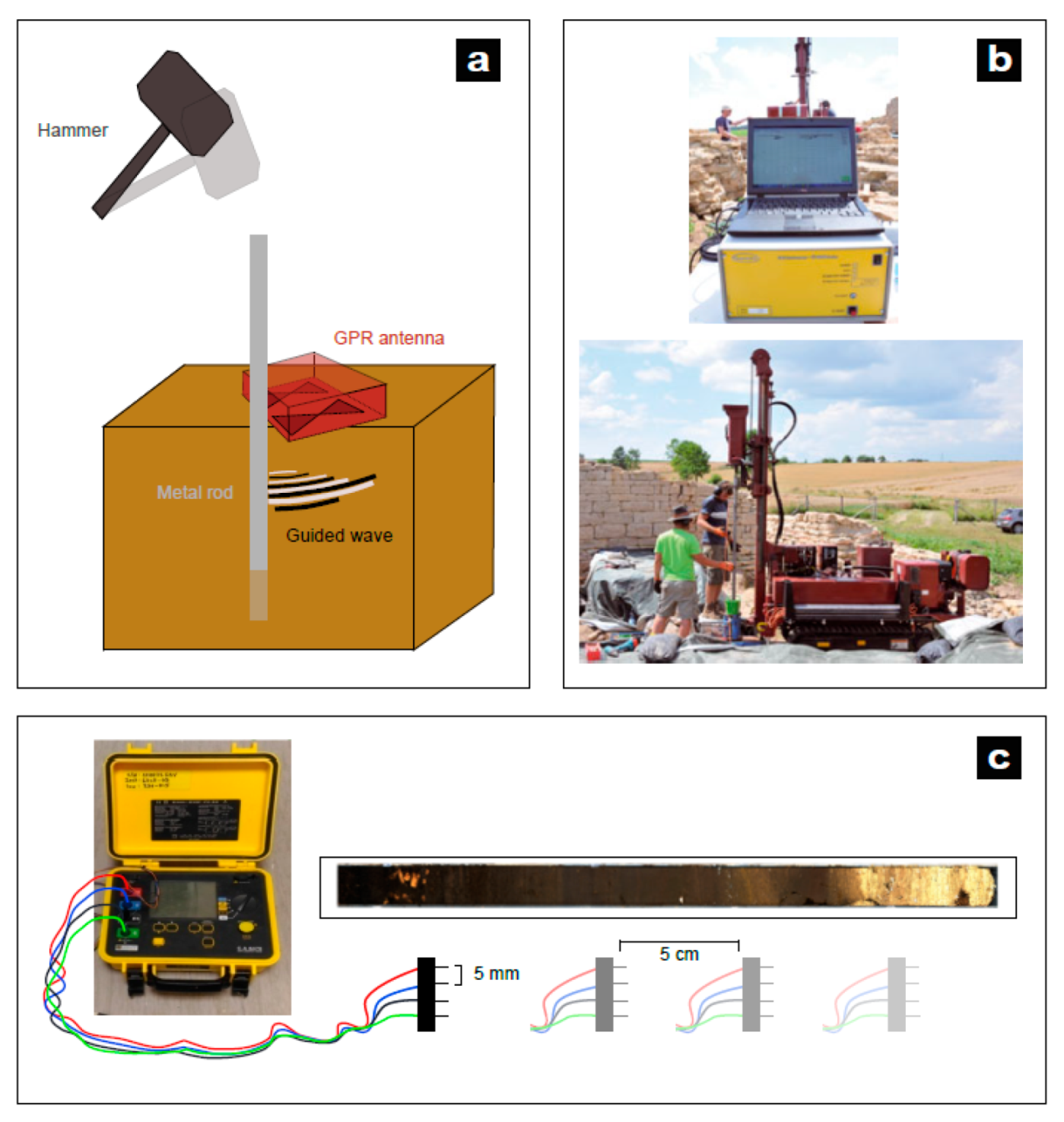
3.1.2. GPR Downhole Profiling Using Guided Waves

An innovative way of measuring radar wave velocities at depth is the use of guided waves in a borehole [56], (Figure 2a). This method yields a continuous record of velocity with a regular downhole spacing of a few cm. In contrast to the familiar CMP-velocity sounding, it is applicable not only to reflecting horizons, but also to gradual velocity changes. Using the same principle as TDR (time domain reflectometry) sondes, the measurement technique uses a steel rod, which is pressed or hammered stepwise into the ground. It serves as a wave guide for the electromagnetic waves emitted by a regular GPR antenna placed next to the rod at the earth’s surface. The waves travel vertically along the waveguide and are reflected at its lower end. Through knowledge of the waveguide’s depth, velocities in each depth interval can be calculated and converted into permittivity values. The innovative technique applied here was developed by the Leibniz Institute for Applied Geophysics [56]. The velocity of the guided wave depends on the permittivity of the investigated deposits, which is strongly influenced by the water content. The two-way traveltime of the reflected wave at different waveguide depths is picked and can be used to calculate interval velocities. We lowered the metal rod into the ground by hammering and recording a GPR trace every 10 cm. The travel times of the reflection at the lower waveguide end were picked and the GPR velocities were calculated. This technique was applied at the three locations of the corings (pink dots in Figure 1).

3.2. Geoelectric Profiling

3.2.1. Electrical Resistivity Tomography (ERT)

A geoelectric measurement is made with a set of four electrodes, the current flows between the two outer electrodes and the potential difference is measured between the two inner ones. Electrode spacing and penetration depth increases during the survey until the maximum spacing is reached, which provides the deepest resistivity information [57].

Geoelectric measurements were conducted using a PC-controlled DC resistivity meter system RESECS (Geoserve) with 96 electrodes. The electrode spacing was 0.5 m (total length of the profile 47.5 m, yellow line in Figure 1) and we measured Dipole-Dipole and Wenner-Alpha arrays. Electrode locations were determined by a Differential GPS (Leica Geosystems AG, Heerbrugg, Switzerland). The inversion was carried out in 2D by applying BERT (Boundless Electrical Resistivity Tomography [58]), a finite-element (FE) inversion software. The starting model is made up using a homogeneous resistivity value of 29.84 Ωm. A regularization parameter of λ = 20 was applied in the standard inversion, that was selected based on the L-curve method (L2-NORM) [59].

The quality of the fit of the resulting electrical resistivity model is given by the RRMS (relative root mean square) deviation between measured and modelled data (in %) and by the chi-squared misfit. The authors of [58] state that chi-squared values of one to five show that results are statistically reliable, meaning that the data are neither overfitted nor underfitted.

3.2.2. Vertical Electric Profiling Using Direct-Push

Direct-Push (DP-EC) logging was conducted using a Geoprobe SC520 soil conductivity probe [60], Figure 2b. The probe is composed of four electrodes in linear arrangements and was operated in a Wenner array enabling a vertical resolution of 0.02 m (www.geoprobe.com; [60,61]). The electric current and voltage are constantly measured with depth and used for the calculation of electric conductivity in mS/m [62]. This equipment was used to measure at the location of core I.4 (orange dot in Figure 1) and the values have been compared also with the measurements carried out in the laboratory.

3.2.3. Electric Resistivity Measurements on Drill Cores

In the laboratory, the electric resistivity of drill core segments was measured using an earth resistivity meter connected with four electrodes in Wenner-Alpha configuration (5 mm long and 5 mm distant with a diameter of 1 mm, Figure 2c). The quadrupole was inserted into the sediment, ensuring the contact between the electrodes and the ground. The surface contact area of the electrodes is about1 mm².Due to the varying sediment conditions, the electrodes had different penetration depths in different layers. This was compensated by applying correspondingly varying geometry factors considering that the electrodes are nearly punctiform. We measured on each core with 5 cm point spacing and compared the measured values with Direct-Push and ERT.

3.3. Seismic Sounding with Shear (SH) Waves

3.3.1. Motivation of Applying SH-Waves in Geoarchaeology

Reflection seismics deals with the use of seismic waves, which reflect at geological interfaces separating layers with different seismic impedance (the product of density and seismic wave velocity). The propagation velocities of seismic waves (P- and S-waves) depend on subsurface composition, fabric, effective ambient pressure and temperature. S-waves are more suitable for near-surface applications in unconsolidated sediments because the propagation velocities are much slower than P-wave velocities, enabling the imaging of geological and archaeological structures with a higher spatial resolution (e.g., [63]). The second aspect is that S-wave velocity and reflection strength are only very slightly influenced by water saturation. Therefore, S-wave velocities often can be more directly correlated with stratigraphy than P-wave velocities. In general, P- and S-waves are coupled due to conversions at interfaces. For 1D layered media, the S-wave is decoupled from the P-wave if the polarization of the S-wave is purely horizontal. In this case, we call the S-wave “SH-wave”. No conversion from S- to P-wave and viceversa occurs. The decoupling of the S-wave is also valid for 2D media if the horizontal polarization is in the strike direction of the 2D media. For investigating the subsurface structure at Duvensee, we applied seismic reflection imaging and seismic traveltime tomography, which are explained in the subsections below.

We conducted a seismic profile, which was oriented in the dip direction of the local underground [31]. We excited S-waves by horizontal hammer blows against a steel bar, which was coupled to the ground by steel spikes. The blow direction was perpendicular to the profile, i.e., in the strike direction of the local underground. Therefore, the excited S-waves were SH-waves. The data were recorded with three Geometrix Geode seismographs, equipped with horizontal geophones. The orientation of the geophones was also perpendicular to the profile. Detailed information about the spacing, geometry and setup of the seismic profile can be found in Table S2. To convert seismograms into seismic reflection images showing depth sections of the stratigraphy, we use digital amplitude processing (called common-midpoint (CMP) processing) and seismic migration. The theory and analysis of seismic reflection data is well documented (e.g., [64]).

3.3.2. Seismic Refraction Tomography

In contrast to reflection seismics, refraction seismics data interpretation aims at determining the spatial distribution of seismic wave velocity as a characteristic of the sediment type. This is executed by analyzing the arrival times of critically refracted waves.

The ratio of the seismic velocity of the layers above and below the refracting interface affects the refraction effect, whilst critically refracted waves only appear if the below layer has a higher velocity than all layers above (in this case, this base is formed by sands).Seismic refraction interpretation requires the identification of refracted arrivals in the seismograms, first arrivals mostly, and the picking of their traveltimes. As a first step, a smooth seismic velocity model of the subsurface has to be derived. This model serves as the reference starting model for a 2D tomographic inversion computation. The result of the refraction tomography is a 2D distribution of the wave velocities representing a depth section underneath the profile line.

For traveltime picking, we used the interactive analysis tool PASTEUP for wide-angle seismic data [65]. The tomographic inversion software Tomo2D [66] was used to derive the S-wave velocity model.

Tomo2D uses a combination of the graphs method and binding method to calculate the ray paths and synthetic travel times. The global difference between observed and synthetic travel times is inverted for velocity perturbation in the underground by solving the linear equation system with a least squares solver. Smoothness constraints and a regularization factor are used [66] to stabilize the inversion. Due to the non-linear nature of the tomographic problem, the difference between observed and synthetic travel times are minimized by iteratively updating the underground velocity model. The applied processing steps are reported in Appendix B.

3.3.3. Seismic Reflection Imaging

The vertical resolution of seismic measurements can be defined as the ability to distinguish between two reflection signals. It represents the distance between two interfaces as separate reflectors, and it is generally determined as a quarter of the dominant wavelength (Rayleigh’s criterion). The acquired data cover a frequency band from 6 to 100 Hz. The seismic data were processed with the VISTA software (https://www.software.slb.com). The observed surface wave (Love wave) is strong. After removing noisy traces, we limited our data to offset smaller than 1 m to ensure that we observe only under critical reflections and therefore no Love waves. We applied filters to enhance the reflections. To compensate the amplitude decay due to the geometrical spreading, an analytic amplitude gain (linear in time) was applied. The velocity model derived in the tomography was used to determine the rms velocity model needed for the Normal-Move-Out (NMO) correction. It was also used for the finite difference migration and for the conversion of the seismic image from time to depth.

Table S4 reports the acquisition parameters (left) and the processing flow with associated parameters (right) used for the seismic measurements and processing at Duvensee. A comparison between the raw and processed data is shown in Figure S1.

3.4. Acquisition of Stratigraphic Data by Drilling and Laboratory Analyses

Corings were conducted using an Usinger piston corer [67], proceeding with 1 m depth increments along a 50 m long transect (blue and green dots in Figure 1), which has been taken as a reference profile. The stratigraphy was described in the laboratory. Moreover, the reconstruction of the transect and a brief description of the main stratigraphic units is given in [31]. Following this, standard laboratory analysis on sediments was carried out:

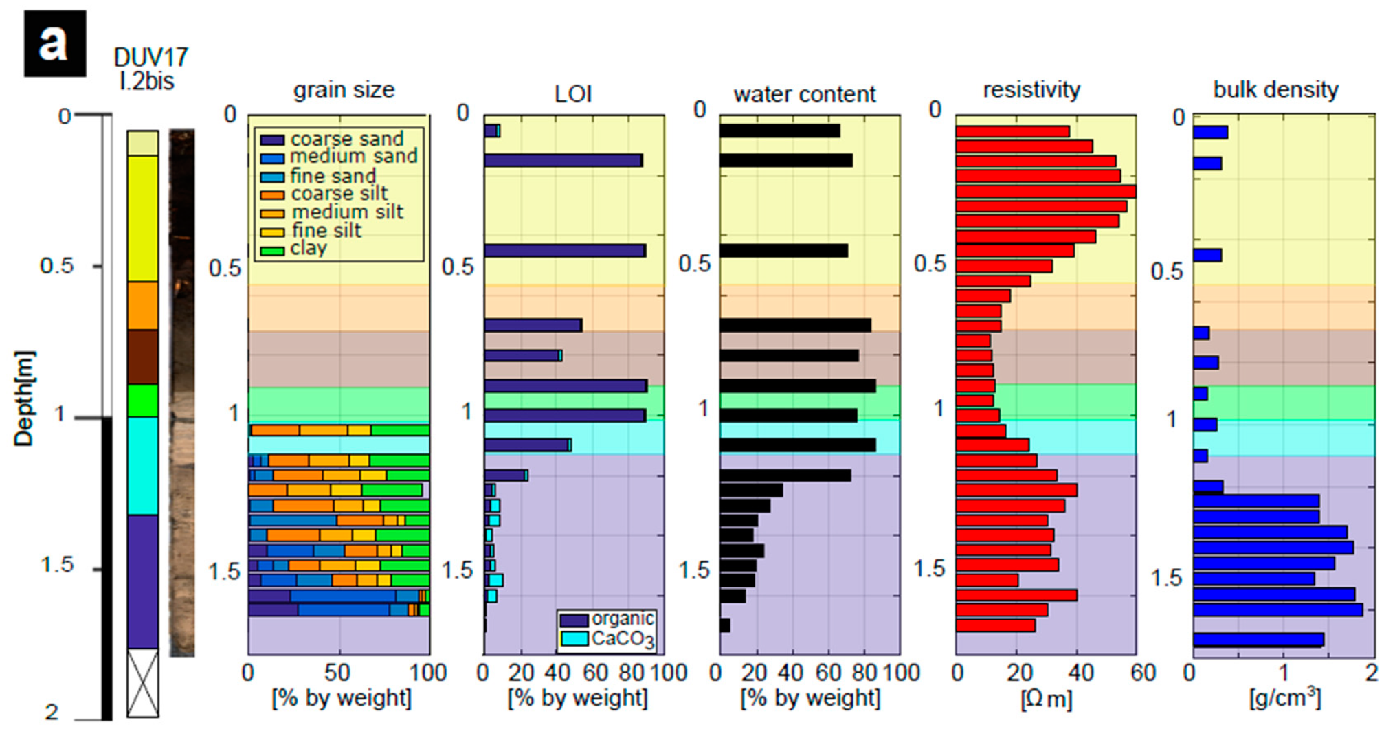
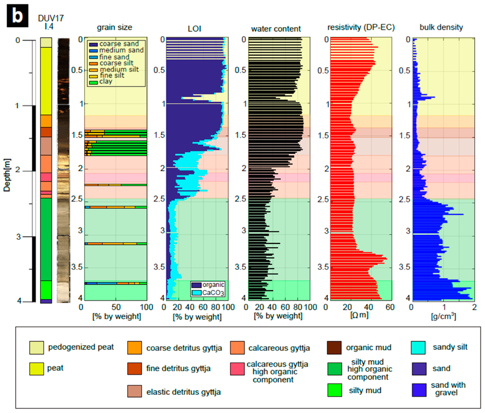
• Water content and bulk density of the sediment samples were determined gravimetrically on small volumetric samples (ca. 2 cm³) after drying the sediment at 105 °C. The sediment of the remainder of the cores was air dried (35 °C), carefully disintegrated with mortar and pestle and sieved through a 2 mm mesh sieve before additional analysis.
• Grain size distribution analysis (<2 mm) was carried out for the sediment of the cores except of the peat layers. After the removal of soil organic matter (H₂O₂, 70 °C) and carbonates (acetic acid buffer, 70 °C, pH 4.8), the sand fractions of the sediment were separated by sieving through meshes of 630, 200, and 63 µm. The silt fractions (2–6.3, 6.3–20, 20–63 µm) and the clay (<2 µm) were separated by sedimentation in Atterberg cylinders.
• The magnetic susceptibility was measured on 10 mL samples (<2 mm fraction) using a Bartington MS2B susceptibility meter (resolution 2 × 10⁻⁶ SI, measuring range 1–9999 × 10⁻⁵ SI, systematic error 10%). Measurements were carried out at a low (0.465 kHz) frequency. A 1% Fe₃O₄ (magnetite) was measured regularly to check for drift and calibrate the results. Mass-specific susceptibilities were calculated [68].
• Loss on Ignition (LOI) values were measured as estimates of the organic matter and carbonate contents of the sediments [69]. After drying the samples at 105 °C overnight, the weight loss of the samples was determined after heating times of 2 h at 550 and 940 °C each.
• Total elemental contents were mesasured on selected samples using a NITON XL3t 900 ped-xrf analyser following the instructions of [70].
• Electrical conductivity of the pore water was determined on the water that sublimated during freeze drying of core samples. Samples were dried separately, and, after the thawing of the ice that formed on the condensator of the freeze dryer, the electrical conductivity of the pore water was measured using a conductivity meter of FA. WTW in µS/cm.

Given the small sample size (half sediment cores of 55 mm diameter), no replicate measurements were possible.

An important remark is needed at this point: coring operations proceeded at 1 m increments in depth. However, the uppermost segments of the cores are sometimes shorter than 1 m. This discrepancy results from sediment compression produced by the extrusion of the sediment out of the Usinger corer barrel. Notably, these compression issues appear to affect only organic layers (peat in particular) in the first meter below the surface. Sedimentary units with a distinct minerogenic or calcareous component are only marginally affected. Understandably, sediment compression affects the measurements of stratigraphic transitions and the estimation of the compression is important also for ground truthing.

4. Results

In the following section, we first show the results by methods starting with the laboratory analysis of cores I.2bis and I.4 and continuing with field GPR, ERT and SH-wave seismic. At the end of the section, we compare and evaluate the results of the different approaches showing their connection for the ancient basin evolution.

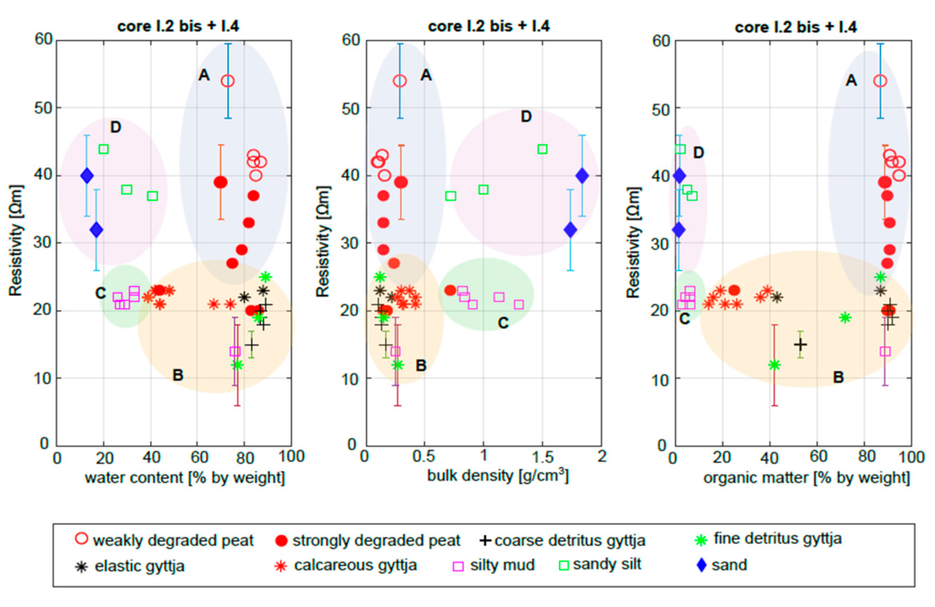
4.1. ElectricalResistivity and Sediment Properties

The results of the laboratory analysis of core I.2bis and I.4 are shown in Figure 3a,b, respectively. An overview of all cores extracted along the 50 m transect (color coded dots in Figure 1) and their stratigraphy can be found in [31]. The sediment properties that are shown are grain size, Loss on Ignition (LOI), water content, resistivity, and bulk density.

Underneath the organic layers, core I.2bis shows an increase in grain size between 1 and 1.7 m of depth, indicating a change from silty sediments to sands at the bottom of the core. The organic matter and water content are high (~80%) from the top of the core up to 1.2 m of depth. Underneath, the organic portion decreases and a corresponding increase in the bulk density occurs (~1.5 g/cm³). This boundary indicates the transition between fine sediments and sands. The electric resistivity shows higher values from the top of the core down to 0.5 m of depth (~50 Ωm), where a decrease in these values down to ~1 m (~15 Ωm) occurs, too. Below 1 m, the resistivity increases again, presenting local variations (~35 Ωm). Based on electric resistivity, the following transitions between sediment types can be identified: the peat on top can be separated from the fine organic mud and silty to clayish-loamy sediments underneath. The second increase in the resistivity corresponds to the presence of sand at the bottom of the core. Focusing on the peat layer, an increase and a decrease (between 0.3 m and 0.6 m) inthe resistivity is visible, which can be correlated with a different degree of humification [71].

Core I.4 (Figure 3b) provides information down to a depth of 4 m. The grain size distribution shows a high amount of clay in the fine organic gyttja layer between 1.5 and 1.8 m. Below 1.8 m, the grain size becomes dominated by silt, and below 3.7 m by higher amounts of sand. The organic matter (~90%) and water content (~80%) decrease from the top of the section down to ~2 m depth with little variations due to the presence of plant remains and wood. The carbonate content increases between 1.8 and 2.5 m (~30%), indicating the deposition of a calcareous gyttja. Below 2.5 m, a decrease inboth components occurs (~10% for organic matter and ~30% for water content) and an increase inthe bulk density (~1–2 g/cm³) is visible, which is associated with the presence of a silty minerogenic mud.

The resistivity values resulting from the Direct-Push measurements show variations that are correlated with different sediment transitions. A first decrease happens between ~0.4 and 1 m depth(from ~40 down to ~20 Ωm) indicating a change in the peat degradation. Between 1.0 and 1.3 m, the values are constant indicating coarse detritus gyttja (~20 Ωm). Between 1.3 and ~ 2 m, the values show little variability, indicating internal changes in gyttjabut making it difficult to pinpoint exact transition depths. Below 2.0 m, the resistivity is constant (~25 Ωm) due to the silty minerogenic deposit, and it shows again an increase at ~3.4 m (>40 Ωm) of depth, correlated to the presence of sandy sediments.

In summary, we can recognize that the peat deposit thickens northwards to the deeper part of the basin, from 0.5 m at the south end to a maximum depth of~1.20 m. The water content is nearly constant, between 80% and 90% and heterogeneities are marked by small decreases. The organic matter content is ~90% with some changes probably caused by the presence of wood remains. An increase inthe bulk density associated with a decrease in the organic matter is also present. The resistivity increases from the top to ~0.4 m depth presenting values between 50 and 60 Ωm, which probably correspond with the poorly decomposed peat. Below this horizon, the resistivity decreases down to 20 Ωm, defining the strongly degraded portion of the peat. The electrical conductivity of the pore water showed a clear gradient. Whereas, in the peat, the values are lower (55 cm–42.3 µS/cm, 65 cm–80.6 mS/cm), there is an increase towards the detritus gyttja (155 cm–254 µS/cm), and even higher values in the calcareous gyttja (220 cm–522.9 µS/cm) and the silty detritus gyttja at the base of the sediment sequence (330 cm–434.6 µS/cm). This might reflect the lowering of the groundwater level in recent times, conducted to make the site agriculturally usable (meadow).

4.2. Ground Penetrating Radar

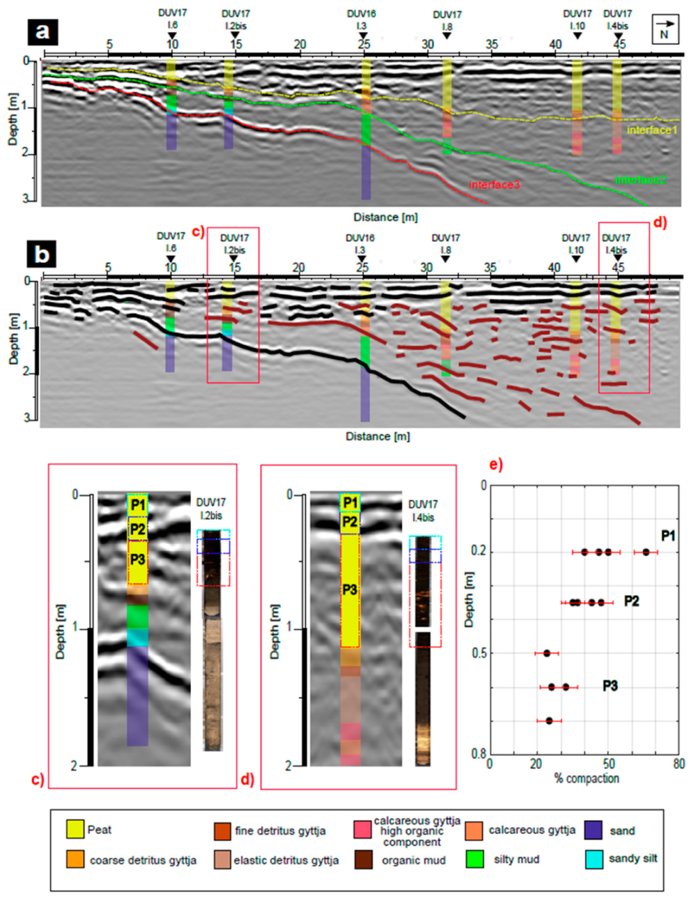
4.2.1. Stratigraphy from GPR Reflection Profiling

In a previous study, we showed that the major stratigraphic units can be traced over the whole 63 ha area of the Duvensee bog by combining drill core analysis and GPR profiling [31]. Three major stratigraphic interfaces showed up as continuous reflections (Figure 4a), which turned out to be caused by changes in grain size of the main sediments. The main units visible in the stratigraphy (Figure 3) are peat (pedogenized peat and decomposed peat), detritus gyttja (coarse, fine, and elastic detritus gyttja), calcareous gyttja, organic mud, minerogenic mud and sand sediments. Therefore, the presented model in [31] consists of four layers separated by the following three main interfaces (from top to bottom):

• Interface1 represents the transition between the coarse organic sediments (peat and coarse detritus gyttja) at the surface and the underlying fine organic sediments (i.e., fine detritus gyttja, calcareous gyttja);
• Interface2 describes the transition between fine organic sediments and underlying clayish-loamy deposits in the bottom of the previous lake;
• Interface3 marks the transition between the clayish-loamy layer and the basal sand deposits.

In between these major interfaces, sequences of internal reflections are visible, which are partly higher, partly lower in amplitude than the reflections from the main boundaries. From the surface down to ~0.7 m of depth, we notice clear sub-horizontal reflections that are locally interrupted. Below 0.7 m, discontinuous, patchy sets of dipping internal reflection elements occur. An interpretation of these features is shown in form of a line drawing in Figure 4b, where the shallow continuous and deeper patchy internal reflections are indicated with black and dark red colors, respectively.

The sets of strong sub-h reflections (black lines in Figure 4b) seem to be confined to the uppermost layer. The inspection of drill cores suggests that these reflections are caused by the transition between the uppermost weakly decomposed peat, showing the highest porosity, and the underlying well-decomposed peat showing lower porosity. The weak internal reflections of the gyttja layer (between interfaces 1 and 2, dark red lines in Figure 4b) do neither follow a clear trend in dipping, nor do they correlate systematically with visible sedimentary changes in the drill cores. Therefore, they have to be considered as scattering caused by small-scale variations in sediment composition originating from the heterogeneity of the deposition, degradation processes and the decomposed organic material.

The internal reflections of the clayish-silty layer 3 basically follow Interfaces2 and 3. The lateral continuity of these reflections indicate that the deposition of layer 3 proceeded more continuously than the deposition of layer 2.

As reported in Section 4.1, the peat water content is usually >80%, which strongly influences the propagation velocity of radar waves and limits their sounding depth to a few meters, in our case due to attenuation (e.g., [72]). Using CMP measurements together with the stratigraphic depths from the corings [31], we defined an average interval velocity and its standard deviation for each main layer: v₁ = 0.045 ± 0.005 m/ns for coarse organic sediments (peat and coarse detritus gyttja), v₂ = 0.039 ± 0.003 m/ns for the fine organic sediments (fine detritus gyttja and calcareous detritus gyttja), v₃ = 0.037 ± 0.003 m/ns for the clayish-loamy layer. We noticed that, close to the surface, the velocity shows values of ~0.049 m/ns, while, in the deeper humified peat, the velocity is ~0.041 m/ns due to the high variability of the water content in the peat sediments. The change in velocities between the gyttja sediments and silty deposits is very small; therefore, the interface reflection of these sediments (Interface2) is weaker than the peak reflection (Interface1). The gyttja layer (between Interface1 and Interface2) shows internal layering of fine detritus gyttja and calcareous gyttja. However, it was not possible to differentiate between these units in terms of radar velocity given the general uncertainty of the CMP measurements. Still, there must be internal velocity variation, as indicated by the sporadic internal reflections. To evaluate it, more refined methods such as full waveform inversion or downhole measurements have to be applied. In this regard, we tested the guided wave technique to improve the velocity determination (see next section). According to the quarter-wavelength criterion, the resolution of the GPR reflection images is about 5 to 8 cm in layer thickness, which means that the different gyttja layers can be distinguished if they exhibit sufficient permittivity contrast and thickness [31].

As explained in Section 3, the compressibility of peat depends mainly on the degree of decomposition. Figure 4c,d show the results of the GPR measurements and an estimation of the compaction for the first meter of the profile after extraction. Referring to [73], we can basically recognize three different degrees of decomposition starting from the top:

(1)

Pedogenized peat (vermulmter Torf) visible in the first 10 cm (P1 in Figure 4c,d);

(2)

Grounded peat (vererdeter Torf) carrying a crumb structure and locally roots, usually concentrated between 10 and 40 cm (P2 in Figure 4c,d);

(3)

Strongly decomposed peat, below 40 cm, (stark zersetzter Torf) with a fine grain structure and wood remains in it (P3 in Figure 4c,d).

Due to the weakness of the matrix, peat layers get seriously compacted if they are sampled by drilling. As a side-product of the GPR investigation, this artificial compaction can be assessed based on the visible reflections and the radar wave velocities of the layers.

Figure 4e shows the results of the compaction estimation regarding the first meter of the corings. The shallower peat (P1 and P2) shows a compaction range from ~40.5 to ~70% referring to (P1), from ~35 to ~50% considering (P2), while the highly decomposed peat (P3) shows an average compaction of ~30%. According to the theory (Section 3), the compaction rate decreases from the top to the bottom of the peat layer considering different degrees of decomposition. Indeed, the high porosity of the top layer creates a higher compaction.

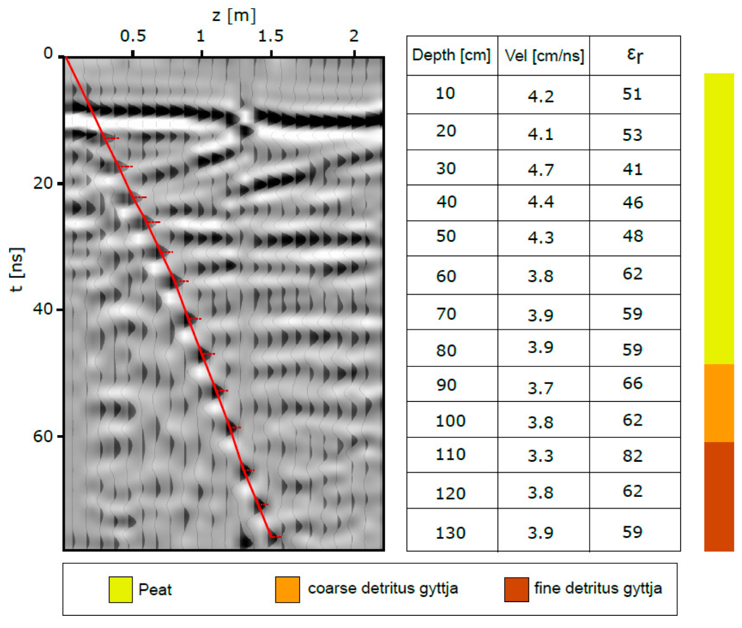
4.2.2. Guided Radar Waves

In this section, we report the results of the guided wave measurements at the location of core I.8.The red line in the wiggle plot (Figure 5) indicates the guided wave arrival, which delivered the velocities listed in the corresponding table in Figure 5. The radar velocity decreases with depth almost continuously with some local change. Focusing on the peat layer, we can notice a higher variation compared with the gyttja sediments underneath, confirming the high variability of peat properties. The gyttjas show instead a smaller variation of the velocity. The resulting average velocity associated with the peat layer is~0.042 ± 0.003 m/ns, which can be well correlated with v₁ as determined from CMP velocity analysis (Section 4.2.1). The same applies for the gyttja, which shows an average velocity of ~0.037 ± 0.002 m/ns consistent with v₂ (Section 4.2.1). This high-resolution test, focused on the determination of the GPR velocity, delivered results that are consistent with the CMP measurements carried out in the same area [31], allowing for the identification of small-scale permittivity variations, which can be correlated with local small and weaker reflections, as reported in Section 4.2.1. Below 70 ns, no arrivals are visible and, therefore, it was not possible to determine the velocity associated with calcareous gyttja and clayish-loamy gyttja. The test at location I.1 was able to deliver the GPR velocity of the sand because the deposit is located already at 0.5 m depth (v₄ = 0.068 ± 0.004 m/ns), which is consistent with the values of wet sand in the literature (Appendix A). The high water content and the presence of the water table can attenuate the radar waves and make the determination of further reflections very difficult.

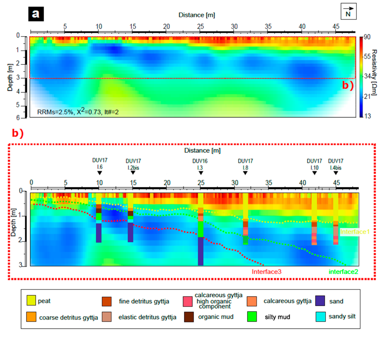
4.3. Electrical Resistivity Tomography

The tomographic inversion of the geoelectric data delivered the electric resistivity model shown in Figure 6. The tomographic computation converged after two iterations showing RMS residuals of 1 to 2.5%. In correspondence to the drilling results three major units can be identified in the ERT model. A uniformly resistive upper layer is visible with a maximum resistivity range of ~60 to 90 Ωm, underlain by a conductive unit of varying thickness (resistivity range ~ 20–35 Ωm). Below this layer, a higher resistive unit of varying thickness is found (resistivity range ~35–50 Ωm).

The upper resistive layer correlates well with the peat deposits confirmed from corings. The relatively high resistivity of the peat is attributed to the low ionic concentration of the peat pore water. The underlying conductive layer incorporates both, the fine lake sediments (fine detritus gyttja and calcareous gyttja) and the Late Glacial minerogenic silty deposits. The high conductivity of the lake sediment is caused by the higher ionic concentration of the pore water resulting from ionic input from the catchment mineral soils. The lowermost layer is defined by an increase in resistivity due to the presence of basal sandy sediments.

The GPR interfaces are superimposed for comparison (dashed yellow, green and red lines in Figure 6b). Interface3 matches very well with the top of the high-resistivity area correlated with the basal sand deposit. Interface2, the top of the clayish-silt layer, is located inside the high conductive unit indicating that the gyttjas cannot be distinguished from the clayish-silt unit by geoelectric sounding from the earth surface. Interface1 correlates well with the high-resistivity upper layer, which distinguishes between coarse organic and fine lake sediments.

In summary, it turned out that geoelectric tomography is able to distinguish between fine lake sediments and basal sand, and between the peat deposit on top and the lake sediments underneath. To better understand up to which degree the different gyttjas can be resolved, we performed the numerical modelling study reported in the supplementary material.

Figure S3a shows a simplified electric resistivity model based on the sediment layers and their depths as derived from the drill cores. To these layers, typical electric resistivity values resulting from the Direct-Push measurements were attributed. For this model, we calculated synthetic geoelectric data, which were then inverted again using the same parameters as for the tomographic inversion of field data. The inversion result is presented in Figure S3b overlain by the GPR-derived interfaces for comparison. The comparison shows that the two uppermost layers (depth <2 m) can be distinguished tomographically, and the inversion (Figure S3b) of the synthetic model (Figure S3a) matches with the tomographic image derived from the field data (Figure 6a). Moreover, a model without the internal gyttja layer was inverted and the results are reported in Figure S3d. Both models agree confirming that the different gyttjas cannot be distinguished. The upper high-resistivity layer can be well associated with the peat deposit. Within the uppermost peat layer, the real data tomographic image (Figure 6a) shows some patchy localized high-resistivity anomalies, which do not appear in the synthetic tomographic image. Therefore, we conclude that these patches are not an artefact of the tomographic computation process, but an indication of lateral inhomogeneity of the upper layer. The gradual transition between the coarse organic sediments and the lake sediments is also visible in the modelling results. Both inversion results agree in showing a gradual transition between coarse and fine sediments probably caused by a coarse detritus gyttja layer ~30 to 40 cm thick, in which the lowering of the resistivity is caused by the presence of a higher ionic concentration. We can confirm that Interface2 is not visible in the model and the sand deposit is clear, but it is less precisely defined. The higher resistivity values of the last layer are more concentrated between 15 and 30 m, but they are at a greater depth and in the first meters are not well defined. The model shows a linear dipping interface, while the GPR interface looks more rounded, this approximation can probably create the misbalance. From the resistivity diagram, we also notice any difference between coarse detritus gyttja and peat above and the lake sediments below it. This statement is also strengthened by comparing the Direct-Push values with the resistivity curve extracted from the ERT results (Figure S4). The computed curve does not show a variation correlated to the coarse gyttja layer. In addition, with the low thickness of this layer and the larger size of grid cells in the ERT model at the same depth, this layer is not visible.

Therefore, we conclude that it is not possible to resolve the difference between coarse detritus gyttja, peat and fine-grained lake sediments (therefore the different gyttjas are not distinguishable).

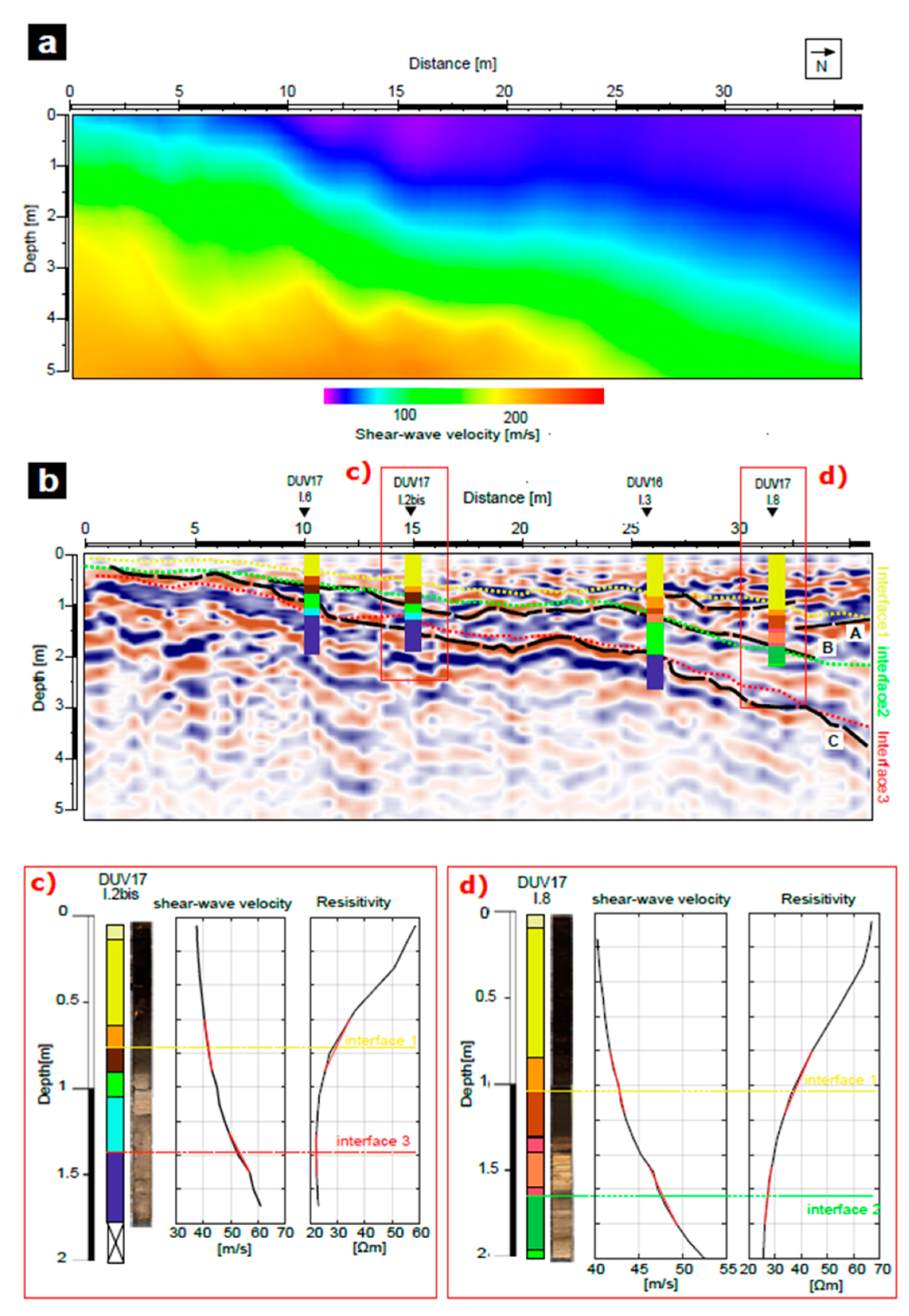
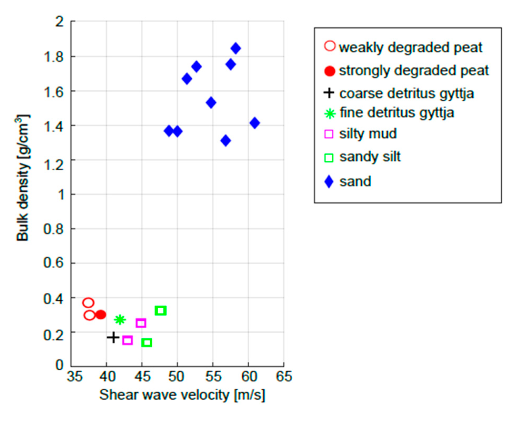
4.4. Shear Wave Seismics

The seismic results are displayed in Figure 7. Both reflection and refraction profiling provide structural information down to about 10m of depth, but, for our purpose, only the first 5 m are considered. The bulk seismic structure can be recognized easily from the depth section of shear-wave velocities (Figure 7a) generated by refraction tomography and from the reflection section (Figure 7b), which allows for a more detailed structural interpretation of the velocity field.In general, the shear-wave velocities increase towards depth with values ranging from 40 to 250 m/s. At the first glance, we can recognize an uppermost layer with velocity <80 m/s followed by two layers with higher velocity values dipping from south to north. The first is characterized by a velocity of ~100 m/s, while the lowermost layer shows velocities ~200 m/s.

The shallower low velocity values are in strong contrast to the lowermost and confirm the presence of a sediment volume at the surface, which is mechanically significantly weaker than its underlying. The observed velocity values <80 m/s indicate soft sediment such as fine-grained lake fills or swampy organic material [23]. It can be interpreted as the sediment sequence of the former lake consisting of peat and fine-grained organic sediments like gyttja and the Lateglacial fine minerogenic sediments.

Below this low-velocity layer, the S-wave velocity increases abruptly to values of 100 to 250 m/s in the vertical direction. The values of 150 to 300 m/s are typical for unconsolidated sediments of varying grain size, basically silt, sand and gravel (c.f. [24,74]).

The spatial resolution of the reflection images can be evaluated using the depth-converted reflection section, from which we can determine the effective wavelengths (Figure 7b). In the upper 2 m of the section, we notice that the wavelength is about 0.4 m, while at deeper levels it becomes wider, ~1.4 mat approximately 4 m depth. This variation is caused by the dominant frequencies changing with depth due to absorption. The higher frequencies are still in effect at shallowest depths and get increasingly absorbed with depth. This consideration shows that the resolution is about 0.20min the uppermost 2 and0.7 m in a depth > 2m. Considering the cores information, we notice that different sediment thickness is less than 0.20 m, which is comparable to the calculated resolution. Therefore, the interpretation of the basin stratigraphy is possible regarding major deposits.

A further comparison between seismic results, GPR and corings is shown in Figure 7b, in which the major GPR interfaces are indicated with dashed colored lines (yellow, green, and red lines). The most striking structure is a dipping reflection starting at about 1 m depth in the south and deepening down to4 m in the North (black line, C). Obviously, this coincides with Interface3 between lake sediment and sand. Interface3 matches with the abrupt increase in S-wave velocity, indicating the stratigraphic change at that depth.

Below this clear reflector, additional seismic events are visible, presenting a similar behavior and still an increase in the shear velocity. The comparison with the stratigraphy allows for the identification of seismic events, which can be correlated to Interface2 (green dashed line from GPR). At a depth of about 1 m, some reflectors are visible matching with the transition between gyttja sediment and the silty clayish glacial deposit (black line, B).

Interface1, between peat deposits and gyttja, shows up in the seismic reflection section, too. It coincides with the ~40 m/s contour line in the seismic velocity section. Within the peat layer, at a depth <0.7m, the resolution of the seismic reflection image breaks down. This is because of interference of reflected and direct wave arrivals. However, the uppermost peat layer can still be distinguished from the underlying peat in terms of shear wave velocity as it is characterized by a velocity of ~40 m/s, which is the smallest value measured along the profile. Some reflectors are present too at a depth of ~1/1.5m at the same location of Interface1 confirming the possibility to detect this limit, too (black line, A).At the deeper peat levels, the S-wave velocity increases to values >50 m/s due to consolidation.

Finally, we can conclude that the main interface in the reflection seismic is caused most probably by layering of sediments with changes in grain size, bulk density, and matrix rigidity with depth.

In Figure 7c,d, we compare the resistivity depth curve extracted from the inversion and the shear-wave velocity depth curve from the tomography. The slope at the main interface depths can give an indication of the gradient for each property. Considering Interface1, the resistivity slope is steeper than the seismic velocity for each core, which means that ERT can better resolve this layer. Interface2 is better resolved considering seismics because the resistivity curve presents almost no slope at this depth. This is also confirmed from the ERT tomography in whichInterface2 is not visible at all. The basal sand deposit is well defined by shear wave velocities, but almost no slope is visible in the resistivity depth curve. In the ERT tomography, it is very difficult to set a clear boundary, which can define the transition to sand between 1 and 2 m (Figure 6b).

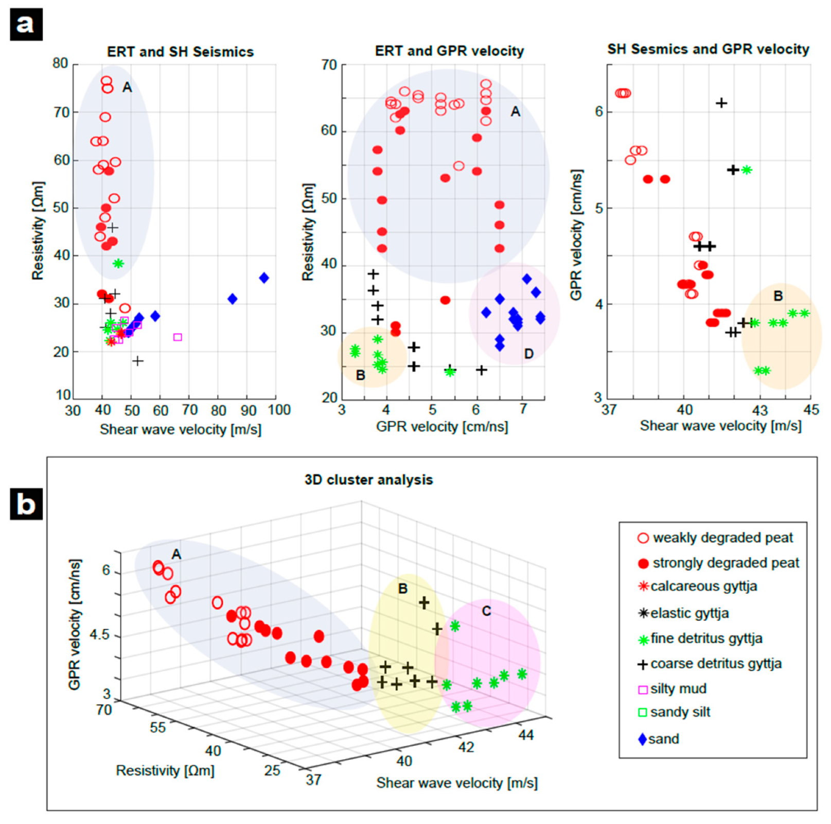
4.5. Comparison of Sedimentological and Geophysical Soil Parameters

In this section, we systematically compare and combine the physical sediment properties determined with the different geophysical methods and with the sediment analysis in order to establish whether or not they can be used to classify bog sediments. The correlation between electrical resistivity and sediment properties is shown in Figure 8 with different symbols for each sediment. In the second part of this section, we combine the physical properties resulting from the computation (Figure 9). Finally, a 3D cluster analysis is presented. For a comparison, we report in Appendix A the values of the sediment properties collected from the literature and in

Table 1. Properties of the peats and gyttjas deposits delivered from this study.

Sediment	Water Content (%)	Organic Matter (%)	Resistivity [Ωm]	Conductivity [mS/m]	εr	SH Velocity [m/s]
weakly degraded peat	66–84	89–95	37–70	27–14	41–53	~40
strongly degraded peat	70–86	87–97	24–40	42–25	59–62	~40
Fine gyttja	86	72	19	52	59–82	~80
Coarse gyttja	87	92	20	50	62–66	~80
Calcareous gyttja	42	17	22	44	n.a.	~80

the results from our study. Moreover, [41] presented a multi-site laboratory study at various peatland sites in north-east Germany, to highlight again the large variability of each property depending on the site conditions.

In the scatter plots of Figure 8, four different clusters are visible: peat (A), gyttjas (B), silty mud (C) and sand (D).Sand, and fine minerogenic sediments are easy to identify as isolated groups. Cluster D shows low water content and resistivity values between 30 and 45 Ωm, whereas cluster C presents low water content and low resistivity values (20–25 Ωm). The situation is different for peat and gyttjas. Peat sediments (Cluster A) have a high variation in resistivity values, but can be clearly separated from the gyttjas, except for some outliers, which have characteristics more like coarse detritus gyttja. The weakly degraded peat is also distinguishable from the strongly degraded peat because of its higher resistivity values. The different gyttjas are not always clearly distinguishable from each other considering the bulk density and water content, the coarse detritus gyttja, fine detritus gyttja and calcareous gyttja belong to a common cluster. The water content enables these paration of the calcareous gyttja from the other gyttja types. A distinction between fine gyttjas and calcareous gyttja is possible in terms of organic matter.

To characterize the correlations between electric resistivity and the other properties of gyttja and peat in a more quantitative way, we applied the Pearson correlation coefficient (r), which varies between 0 (no) and 1 (perfect correlation). Water content and organic matter have the strongest correlation with resistivity, particularly for the coarse detritus gyttja (r = 0.88 for water content and r = 0.87 for organic matter). For peat, we obtained r = 0.32 for the water content and r = 0.58 for the organic matter, they are weaker and probably explained by the high variability associated with this type of sediment. The high variation of this property is site dependent and our results are in line with [18]. The fine gyttjas show a value of r = 0.78 for the water content and r = 0.67 for the organic matter. Coarse detritus gyttja presents similar characteristics to strongly degraded peat, which makes it somewhat difficult to distinguish them.

Figure 9a shows scatter plots of the geophysical parameters obtained from the field measurements’ interpretation. Electrical resistivity and shear wave velocity from the tomographies (uppermost 3 m) are able to distinguish between different degrees of peat degradation (Cluster A). The gyttjas are concentrated in one cluster and show similar characteristics as clayish loamy sediments. The plot of electric resistivity versus GPR (uppermost 2 m) velocities reveals different clusters, particularly the differently degraded peats (Cluster A). The weakly degraded peat is concentrated on the top of the plot (resistivity values ~65 Ωm, GPR velocity 4–6 cm/ns), which makes its identification possible. The strongly degraded peat shows a high variability of both resistivity (~40–60 Ωm) and GPR velocity (4–6.6 cm/ns). Despite its high variability, this sediment is well separated from the others. Some outliers are located close to the detritus gyttja, which makes it difficult to well separate this sediment from the strongly degraded peat and fine detritus gyttja. The sand (Cluster D) and fine detritus gyttja (Cluster B) are more concentrated in separated clusters. In this regard, the fine detritus gyttja could be separated from the coarse one. In the scatter plot of seismic and GPR velocity, we notice that the different clusters can be identified, too, but they show some overlap. Only fine detritus gyttja seems to be concentrated within an isolated cluster (Cluster B).

Combining the three geophysical parameters, a 3D cluster analysis was performed and the results are shown in Figure 9b. Cluster A indicates the peat deposit, which can be distinguished in two subclusters: weakly degraded peat and strongly degraded peat. Moreover, it is promising that the different gyttjas (coarse and fine) seem to belong to different groups (Cluster B and C). Unfortunately, the other sediments are not inserted because it was not possible to measure the GPR velocity below a depth of 1.3 m.

In summary, the identification of different degrees of peat decomposition is possible considering sediment and geophysical properties. The detritus gyttja is often displayed as having similar characteristics to the strongly degraded peat, but the 3D cluster analysis shows that it is possible to distinguish it. The same is true for fine detritus gyttja, which belong to a different cluster.

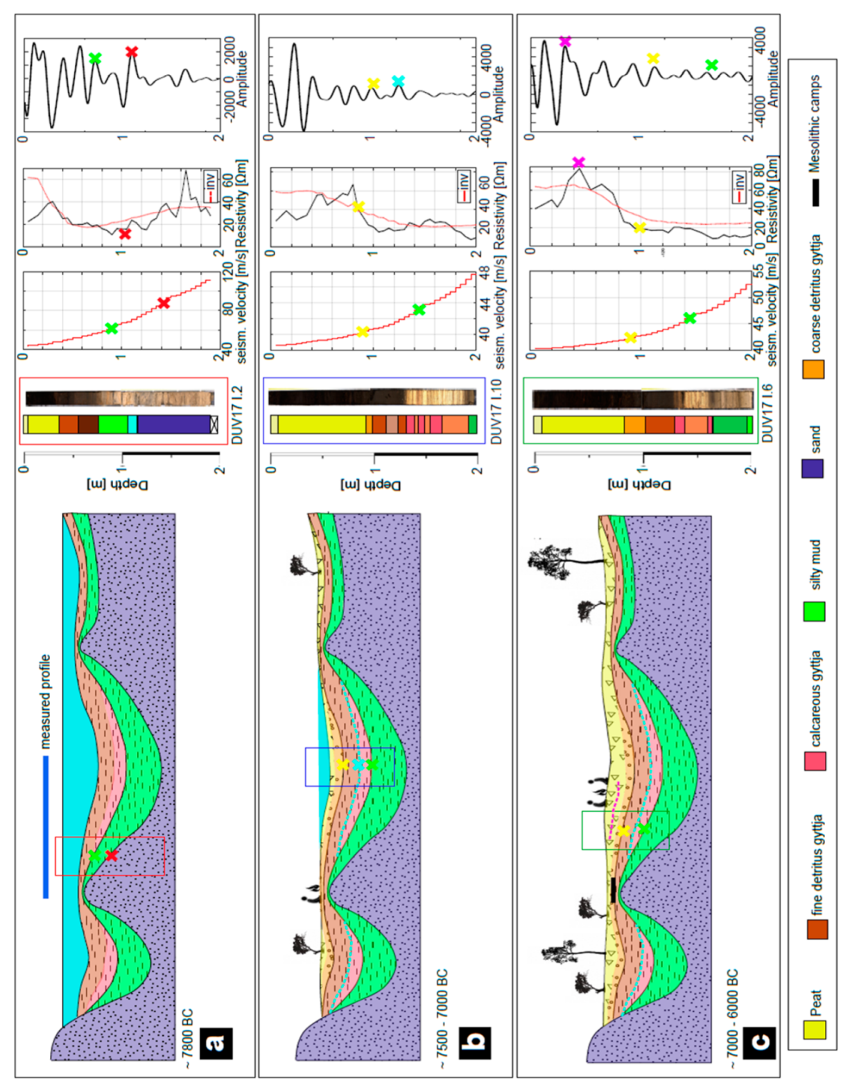
4.6. Peatland Development

The basin stratigraphy and morphology inferred from the geophysical results can be explained in terms of the classical phases of peat bog formation confined in a basin. The initial basin was composed of glacial sands where, above it, Late Glacial clayey silt was deposited in a lake (Figure 10a). The applied geophysical methods can identify the glacial sands characterized by low conductivities compared with the surrounding fine sediments. During the Early Holocene warming, organic-rich lake sediments were deposited, and peat formation began at the lakeshore. By a rapid filling of the lake basin, that occurred already during the Early Holocene, the peat covered a successively larger area of the former lake (Figure 10b,c). In the lake basin, the sequence is more complicated due to the fluctuating water levels during the Preboreal to Boreal, but this sequence is (normally) the common deposition series [52]. Due to the multimethod approach, we were able to identify almost all the stratigraphic units. The basal sand is very easy to identify and to map for the identification of former islands with Mesolithic occupation [31]. Figure 10a shows how this interface (Interface3) is visible in each applied method (red cross), allowing for a reconstruction of the ancient basal deposits. The late glacial clayey silt and the peat unit on top were mapped as well, allowing a first reconstruction of the lake development. Figure 10a–c (green cross) highlights how Interface2 was detected mainly by GPR and seismics because of the low contrast in electrical resistivity between fine lake sediments and the Late Glacial clayey silt. Interface1 (yellow cross, Figure 10a–c) is visible in each method and it can be connected with the bottom of the peat layer, often correlated with coarse detritus gyttja presenting similar properties. Between Interface1 and Interface2, different gyttja sediments (fine detritus gyttja and calcareous gyttja) are visible from the stratigraphy but are not clear in the geophysical results. Some changes in the GPR amplitude are visible (cyan cross, Figure 10) but without a regular behavior that allows for the identification of a defined layer. The calcareous gyttja is visible only in the deep part of the ancient lake but geophysically it does not differentiate from the surrounding lake sediments. The identification of this layer would be important also for timing aspects in a way to better understand the sequence of deposition. Sediment analysis helps the distinction of this layer from the others but, from the geophysical point of view, it is still not defined. The transition between coarse detritus gyttja and peat is also not possible because this sediment presents some similarities with the strongly degraded peat. This is also visible comparing the resistivity curves form the inversion with the measured resistivities in the cores (dashed red lines in Figure 10). In this regard, we can highlight the possibility of separating strongly degraded peat from weakly degraded peat (pink cross in Figure 10). This is an important achievement which can be used for the archaeological research (e.g., preservation conditions of organic remains). As reported in [18], gyttja layers at the base of peat deposits that can often be found in fens of north-east Germany reduce the contrast in electrical conductivity; thus, the delineation of peat is not that clear anymore. The former islands had already started to become overgrown with peat during the Early Holocene, and the Mesolithic camps are indeed not directly located on the mineral soils but embedded in peat. Having more detail about the first layer can be particularly important for further research because it hosts the archaeological record. Our proposed scheme of the stratigraphy is based on the detected units and not on the time of deposition, because this topic needs another approach (e.g., including dating) [31]. A suggestion of the measured profile location is proposed in Figure 10.

5. Discussion

5.1. Stratigraphy of Bogs

5.1.1. GPR Survey

The results of the presented research together with the work of [31] provide vivid information regarding the development of the paleo-landscape at the ancient Lake Duvensee. Physical properties and geophysical investigations helped gain more details about the characteristics of the sediments.

GPR is able to detect different layers at ancient Lake Duvensee, in particular Interface1 (transition between peat, coarse detritus gyttja and the underlying fine detritus gyttja, calcareous gyttja), Interface2 (fine detritus gyttja and underlying clayish-loamy sediments), and Interface3 (transition between clayish-loamy layer and the basal sand deposits).

Conductivity and permittivity are strongly influenced by water and clay content; these properties increase with increasing clay and water content [76,77]. Since permittivity and velocity are indirectly proportional, an increase in those properties means a decrease in the velocity of the electromagnetic waves [76]. Clay minerals are also negatively charged and, therefore, able to exchange cations, if they are in solution [78]. The result is that an additional surface conductivity is present, increasing the bulk conductivity for clayey sediments. Fine organic particles can have similarly high cation exchange capacities than clay minerals but usually exhibit a lower bulk density.

For the reasons illustrated above, Interface3 is well visible in the radargrams, marking the transition between clayish-loamy sediments and sand [31]; this transition is also confirmed considering the organic matter content, which decreases quickly from 30% to <5% at about 1.2 m of depth in core I.2 and also considering the change in water content and bulk density. The bulk density is higher, and the porosity is smaller, reducing the water content, which causes a visible reflection. Organic matter influences the propagation of the radar waves too, because a high value of it enables higher water contents due to the larger surface of particles where water can adhere [79]. Therefore, the permittivity increases in sediments with high organic matter.

Interface2 is also recognizable because of a significant change in organic matter content at about ~2.5 m in core I.4 (from ~30% to ~10%) associated by a change in bulk density. The grain size distribution indicates a change in the clay content which is higher considering the gyttja than the clayey silt below this limit. The reflection is (indeed) weaker compared to Interface3, but it can be followed through the profiles.

Interface1 is instead very difficult to follow without stratigraphic information because the reflection amplitude is somewhere weak and GPR seems to encounter difficulties detecting the transition between different sediments. In the first meter of I.2bis and the first 2 m of I.4 the water and organic matter content do not present large variations. The resistivity can instead give more information about the first recognizable interface because a change of that property occurs at ~0.7 m, defining the transition between peat/coarse detritus gyttja and organic mud in core I.2. and the same for I.4b. A small variation is also present concerning the grain size between coarse and fine sediments.

In the peat layer, discontinuous scattered reflections are present too, which are caused by the heterogeneous character of the peat and it poses a challenge in interpreting reflections within peatlands. Chaotic reflections can be caused by small-scale variations in the degree of decomposition, peat type or wood remains as well. The transition between fine gyttjas and calcareous gyttja has the characteristics to be detected as well, but, in the radargram, we can only see scattered weak reflections (Figure 4). The grain size slightly varies between the two deposits and the organic matter varies too, but more information about the GPR velocity variation would help in this direction.

Regarding GPR, we confirmed that the velocity of electromagnetic waves and therefore dielectric permittivity through peat can be highly variable. Compared to former studies in wetlands, our results fit well with that found by [25,32] for fen peats. The authors of [25] demonstrated that the degree of waterlogging does have an impact on the dielectric permittivity in fen peat; for this reason, the range of variability on peat deposits is very high. Measuring in different seasons can also be a factor that can affect the results, dry conditions give a higher value of the electromagnetic wave velocity than wet conditions [25] as well as the temperature variations.

From the values found in the literature (Appendix A), we know that clay- and silt-rich minerogenic sediments have lower dielectric permittivity than (any of the) peat deposits. Both peat and clay deposits are fully saturated, and the peat has the capacity to hold more water than coarse grained minerogenic sediments due to the pore structure of the sediment [11]. The authors of [25] found an electromagnetic wave velocity of 0.05 m/ns (dielectric permittivity of 36) for the silty to clayey wetland sediments and they are at the upper end of the range given by [34]. Our results are even lower (velocity of 0.039–0.037 m/ns) compared to the literature, probably due to the high water content, which slows down the radar waves.

The guided waves method gave results that are consistent with the CMP measurements reported in [31] and in the literature (Appendix A). Moreover, it delivered higher-resolution information about the variation of the radar velocity in the uppermost 1.3 m. Indeed, these methods allowed for the determination of the GPR velocities every 10 cm. Unfortunately, the high water content of the subsurface made it difficult to gain mode detail at a major depth. Therefore, only peat, coarse detritus gyttja and fine detritus gyttja were reported.

In summary, it is evident that the ability of GPR to delineate structures within the organic deposits depends on the site-specific stratigraphy. It depends on the layer differences in peat type, the degree of decomposition, water saturation, the type of gyttja and small-scale variations in physical properties. Therefore, it is difficult to define general implications for other sites. A step forward would be to use small scale information as constraints [24,60] to improve and validate the geophysical models to be able to predict the stratigraphy and (maybe) define their characteristics.

5.1.2. ERT Survey

The tomographic section of the resistivity shows regions of varying resistivity, which were associated with the major sediments. Within the peat layer, high-resistivity regions are visible, but they cannot be explained by distinct layers. Interface1 was difficult to follow in the GPR profiles but with ERT, it is very clear. The local variations (red spots in the uppermost 1m) are probably associated with the different peat decomposition, which creates differences in the cation exchange capacity, but this is not supported by the statistical analysis of samples. Another explanation for these variations may be a different soil moisture. The statistical analysis of the sample indicates a slight correlation of water content and resistivity providing evidence for this explanation. The decrease in the resistivity within the peat layer is a good indicator of a different degree of humification of these deposits according to [8].

The transition between peat and coarse detritus gyttja is gradual considering the resistivity curve, which does not show an evident change. The detection of gradual changes in property is well documented for ERT in comparison to GPR. The authors of [80] used both approaches to investigate peatland sites and identified regions of varying resistivity within peatland, which could not be resolved by GPR. Thus, we concluded that a gradient layer with continuously changing dielectric permittivity was present, which cannot be detected by GPR.

With respect to the gyttja layers, ERT fails to differentiate between the different types of gyttja. The resistivity of the gyttjas is not significantly higher than the resistivity of the mineral deposits. A masking effect of a high ionic concentration of the permanent groundwater body that fills the pores of this section of the sediment sequence could explain this observation. According to modern times, the lowering of the groundwater level, the upper part of the sediment sequence (peat), is not connected to the permanent groundwater level anymore. This is indicated by the much lower conductivity values of the pore water of the peat compared to the lying gyttja layers. Instead, parts of the pore water of the peat might originate from rainwater, explaining the much lower ion concentrations of the peat.

5.1.3. SH-Wave Survey

The presented refraction tomography and reflection profile have shown different velocity variations and reflectors corresponding to the change in grain size of the sediments, like GPR. The identification of the silty-clay/basal sand is very clear in both methods while concerning Interface2 and Interface1 only partial reflectors are visible. The match between these seismic events is visible, but further measurements would confirm this hypothesis. The incredibly low shear wave velocity at the top of the profile indicates that swampy sediments are very well correlated with the organic peat deposit. The high velocities at the bottom of the section are instead clearly correlated with sand sediment. However, the organic matrix as such is mechanically weaker than the matrix of inorganic sandy and silty soils. Therefore, the related contrasts in shear rigidity (shear modulus) are one of the reasons why shear wave sounding turned out to be successful in determining the shape of the former island. Moreover, the shear wave velocity, which is proportional to the square root of rigidity, is determined mainly by the matrix and is not affected by the pore fill, making SH-wave contrasts independent by the degree of water saturation.

This is very much in contrast to electric conductivity and dielectric permittivity, which are essentially determined by the soil water content. In our field example, the general increase in water saturation with depth led to decreasing lateral contrast between the island and the surrounding lake sediments. For the same reason, GPR absorption increases strongly with depth.

Site effects primarily depend on the shear modulus of layers, which is also related to density. Attempts have been made to propose a relation between the bulk density and shear wave velocity [81,82], and our case study is in line with the literature giving a correlation factor of r = 0.85 (Figure 11).

Focusing on Figure 11, we can notice that the sand deposit is well isolated from the rest of the sediments. At a first glance peat presents the lower velocity values and it can be separated from the fine lake sediments and gyttja, but more data would be necessary to implement that.

Efforts have been made to propose a general trend between shear wave velocities and porosity, permeability under different environmental conditions. Due to the different arrangement and composition of grains, there are differences in density, porosity, and permeability as a result of differences in shear wave and compressional wave velocity. In particular, the higher the density, the lower the porosity and thus the higher the wave velocity [82].

5.2. Degradation and Compaction of the Peat

As we presented in the paper, the extrusion of the sediment from the Usinger core barrel can lead to a strong compaction of the core. In our case, the compaction affected only the first layer made up of peat and coarse detritus gyttja, while the minerogenic and calcareous sediment were marginally or not affected. Taking the depth of the main transitions from the GPR survey in [31], a more focused estimation of the compaction has been done also including the degree of decomposition of the sediments. As we can see from our results the estimation of the compression through the peat is quite variable but combining the sediment parameters with geophysical results (GPR in our case) can give a promising methodology to understand more about this topic. In any case, more tests are needed to understand how peat can be compressed during core extraction.

Another important remark about in-situ peat compaction regards its contribution to total subsidence, which influences temporal and spatial sedimentation patterns.

The work of [12] found no evidence of an easy way to access peat compressibility. They argue that peat from different locations exhibited different compressibility characteristics and they concluded that more commonly and relatively easily measured sediment parameters (e.g., bulk density, state of decomposition) are no proper indicators of soil compressibility. In any case, peat is a highly compressible material and consequently the water storage changes produce volume changes in the peat.

Where changes in water table elevations are large, significant storage changes may arise from surface elevation changes. The nature of the surface elevation change depends on the compressibility of the peat [83].

So far, peat compaction has mainly been quantified using empirical models [84], resulting in estimated compaction rates in Holocene alluvial sequences (about <2 mm/year). However, these results should be verified with field data. The authors of [85] tried to estimate the rate of peat compaction at the Rhine–Meuse delta using bulk density and organic matter and radiocarbon dated peats. He presented a subsidence of up to 3 m in a 10 m thick Holocene sequence (0.6 mm/year), comparing the dry bulk density of compacted and uncompacted peat with an estimated error of about 15%. He also found that, in two of the four cases, the LOI and compaction are positively correlated, but no rule is possible to define.

The degree of decomposition determines the physical properties of peat, too. Undecomposed peat has a low bulk density and high fibre content [8]; therefore, it contains many large pores and may have a total porosity of~97%. During the decomposition, peat becomes denser and its porosity reduces to 81–85% for strongly decomposed peats [37]. In theory, if peat is fully water-saturated, the undecomposed peat has a higher water content and ε_r; thus, the GPR velocity is lower compared to the decomposed one. In our case study, the water content is almost constant in the peat deposits, which means that higher velocities on the top are caused by organic undecomposed materials that can increase the velocity values. As a result of the dual-porosity character of peat, the immobile region presents a negligible fluid flow velocity that can be translated in a decrease as well as the resistivity. Our study reveals this relationship, as we can see from Figure 5, in which the lowermost peat presents lower GPR velocities indicating the more degraded part. This behavior is also confirmed considering the electrical resistivity which decreases with depth in the same sediment according to [8]. In any case to prove this suggestion, additional GPR data against decompositional types of peat is needed.

The degree of composition of peat will also vary according to the plant species making up the peat [11]. Peats containing vascular plant remains often are more decomposable than those containing Sphagnum remains [86]. The pattern of lower and higher permeability peat in the deposit can be expected to affect the water flow through the peat which in turn may affect the patterning of vegetation. Such trends have been explored by [87,88], who showed that complex patterns of vegetation and of peat transmissivity may emerge from relatively simple interactions between vegetation type and water table position. However, a problem of these studies is that they have not been tested with field data, and sometimes the number of boreholes is too small to also understand horizontal variations.

To test models and to find correlations, it would be very useful if the peat could be mapped non-invasively and in detail over large areas. In these regards, GPR can be the best cost-effective method to apply.

In wetland contexts, the fluctuating water table interacting with the sediments and any underlying or overlying depositional material also plays a role. In our case, we do not have information about the depth of the water table, which would help us to understand the depth of penetration of GPR. An estimation can be done considering the geochemistry and the iron concentration, which is expected at the maximum height of the water table. Below this limit the iron concentration decreases with depth due to the sensitivity to redox state and pH in bogs [89]. High concentrations of aluminum indicate a certain amount of minerogenic input into the lake basin from the catchment area. The Late Glacial to Early Holocene lake sediments of the lower part of the sequence expose clearly higher amounts of Al. This reflects a considerable minerogenic input from the catchment area, probably enabled by a sparse vegetation cover on the catchment soils. Towards the upper part of the lake sediment sequence (between 2.3 and 1.9 m) the Al content decreases dramatically, indicating a trend of stabilization of the catchment surface by the succession of a vegetation cover in the lake catchment area. One later phase, that divides the peat deposition, is characterized by high minerogenic input, too. This might reflect a re-opening of the catchment vegetation caused by natural processes, e.g., Early Holocene climate variability (e.g., [90] or local human activity. Copper and zinc are indicative for redox processes at the water table [25]. The high concentration of iron associated with high values of copper and zinc at about ~1.10 m depth (Figure S5) indicates the presence of the long-term mean water table at this depth.

5.3. Methodological Questions

To reconstruct the stratigraphy at ancient Lake Duvensee, a multi method approach has been used in a way to understand which method can deliver the best understanding of the layering.

Soil parameters have been implemented to cover small-scale variations. In the following subsection, we are first going to discuss which method was the most successful for the research foci and what can be improved to better define the stratigraphy. At the end of the section, we will discuss what soil and petrophysical parameters are suitable for identifying different sediments. The fen basin is successfully delineated with GPR and ERT due to the high contrast in electrical properties between the organic and the surrounding mineral basal deposits. SH-wave seismics can recognize and separate the layers that differ in seismic impedance and grain sizeas well. GPR and seismic tomography display sharp interfaces, whereas ERT shows gradual transitions, and these methodical differences are described by other authors as well [28,91]. The investigated peatland is embedded in low conductive glacial sands typical of fens in northern Germany [41], which means that the electrical conductivity of the organic deposits (peat and gyttja) is higher than that of the surrounding material. The delineation of peatland deposits with GPR is more achievable, and, in our case, we were even able to differentiate a different degree of decomposition of peat and somewhere some weak reflections were correlated to different gyttjas (fine detritus gyttja and calcareous gyttja).

We propose SH-wave seismic as an alternative tool to investigate the stratigraphy of such environments. In this regard a comment about the resolution of GPR and S-wave Seismic is needed. GPR shows a resolution between 5–8 cm (Section 4.2), while Seismic 20–70 cm. Concerning the goals of this research GPR would be the best method to use for reconstructing the shallow subsurface and to try to identify also internal layering concerning different gyttjas. The interpretation of the very shallow subsurface (first meter in particular) is very difficult with reflection seismic because of different factors, for instance, it is difficult to separate direct waves, surface waves and shallow reflections in the near field close to the source. This makes GPR more suitable for detecting shallow interfaces. However, seismics is also sensitive to sediments that differ in grain size and it provides information about the density and compaction of different deposits. The depth of penetration differs significantly, making seismic more suitable for surveys focused on the ancient lake bottom. Interface3 is, indeed, very clear and it can be followed in higher depth than with GPR. In the center of the ancient lake, for instance, the core information shows that the sand layer lies at a depth of about 6 m which is difficult to reach with GPR. The authors of [11] used a 200 MHz antenna achieving a depth of 3 m, also enabling the extension of the different peat humifications possible. The authors of references [16,20] used a 50, 100 and 200 MHz antenna, claiming that the second was the best compromise between depth of investigation and resolution reaching a depth of about 10 m having a peat layer of about ~4 m on top. Using antennae of 50 MHz or 100 MHz means that the resolution with S-wave Seismics can be comparable but the depth of penetration would be always more for seismic. For this case study, the best choice would be to keep measuring with a 200MHz antenna; otherwise, with a lower central frequency antenna, we would lose resolution, which could be useful for layering interpretation. However, some improvements can also be planned regarding seismics. The distance between the receivers can be reduced to 0.25 m, but the time of measurements will increase, losing the cost-effective character of the survey. Another remark to make would be about the source used for seismic waves. A higher frequency source would produce waves with smaller wavelength and therefore the resolution would be higher, but, in the SH-wave case, the higher frequencies would be quickly attenuated and difficult to measure.

Moreover, compressional waves (P-waves) can be a tool to test in this case study despite the longer wavelength and thus coarser resolution compared to shear waves. Nevertheless, P-waves are dependent on the compressional modulus and this might be a parameter that is changing between sedimentary layers, too. For example, V_p increases with a decrease in porosity, and increases with an increase in density.

The Full Waveform Inversion (FWI) is a recent tool which is able to improve the resolution of seismic data. At the Fossa Carolina FWI was able to improve the definition of the canal basement and to resolve small-scale velocity anomalies correlated with features in the archaeological documentation [47,48,92]. A further application of this tool could foster the identification of shallow structures and improve the understanding of the seismic signals visible in the reflection profile. The multichannel analysis of surface waves (MASW, e.g., [48,93]) and spectral analysis of surface waves (SASW) can also be used to improve resolution for mapping subsurface stratigraphy.

Magnetic measurements are also common in geoarchaeological research, but, in our case, it did not provide satisfying results. The magnetic susceptibility was measured along the core I.4 and the results are shown in Figure S4. The survey pointed out that between peat and gyttja sediments the magnetic susceptibility does not present any variation. The only visible change is the transition between the calcareous gyttja and the underlying clayey silt deposits, which is already visible with GPR. Therefore, we decided to neglect a survey of magnetic susceptibility. We tested Electromagnetic Induction instead (EMI), and the result is shown in Figure S4. The EMI inversion shows a high-resistivity layer at the top of the profile which can be associated with the peat layer. Underneath this unit, a high conductive area is present correlated to the lake sediments. The identification of the sand deposits is difficult because of the low instrument depth of penetration. For future investigations, the use of EMI with higher depth penetration, e.g., by using an instrument with larger coil spacing, is promising.

Combining geophysics and soil characterization is currently required to aid the rapid discovery and characterization of buried wetland archaeology. For instance, the identification of different peat degradation can be an indicator of the layers preservation which can address the archaeological research. The characterization of the deposits prior to a full survey is therefore an essential step in conducting geophysical surveys in wetlands. We presented a range of different parameters (e.g., dielectric permittivity, resistivity, and SH-wave seismics), which, connected with soil information (water content organic matter), can delineate different deposits. The dielectric permittivity is well defined using the guided wave measurements, which can be improved by also using a motor pulling the metal rod into the ground allowing a more detailed survey of the GPR velocity. Evaluating with more accuracy the degree of decomposition of peat for instance would help the determination of soil compressibility and porosity. Using Direct-Push is the most successful way to determine the conductivity/resistivity values.

6. Conclusions

To study the landscape development of the early Mesolithic sites of ancient Lake Duvensee, a multi-methodological approach has been applied. Fens of the temperate zone of central Europe are still not studied frequently with these methods. The combined use of different geophysical methods (GPR, ERT and SH-wave Seismics) and stratigraphic information from corings helped finding additional information about the stratigraphy of the former lake. Special attention is given to the investigation of different types of gyttja, which can often be found at the base of peat deposits in this region. Based on our field survey, we found that the ancient lake basin prospection can be performed with different methods, each of them sensible to different variations of physical parameters:

• GPR can identify the main transition between sediments that differ in grain size, and the boundary between the uppermost poorly decomposed peat (“acrotelm”) and underlying well-decomposed peat (‘’catotelm’’). Moreover, the distinction between different gyttjas is locally visible with small scattered reflection but without an orientation.

Internal GPR velocity variations, which are represented with sporadic reflections, can be detected using the guided wave measurements, which provide a high-resolution image of the permittivity in the subsurface.

• ERT is capable of distinguishing between sediments with different grain sizes but is not able to distinguish between different fine-grained lake sediments; therefore, the different gyttja types are not detected. However, depending on site conditions, ERT is able to indicate regions of gradually changing properties, such as the solutes in the pore fluid. Perhaps the high ionic concentration of the permanent groundwater body present in the lower part of the ancient lake basin is masking differences in sediment properties. The small-scale variations, due to different degrees decomposition and organic remains, in the peat layer were visible as resistivity changes.

Moreover, using GPR together with stratigraphic information was useful to estimate the peat compaction due the extraction after drilling. It turned out that the compaction is higher for the shallower peat layer associated with the weakly degraded peat, while the underlying more degraded peat presents a lower compaction. But no trend was observed.

We proposed SH-wave seismics as alternative tool for investigating wetlands and it delivered the following results:

• SH-wave seismics enables exploring the deepest stratigraphy (up to ~19m depth), in which the major interfaces can be found from the S-wave velocity distribution as provided by refraction tomography. The method can distinguish between sediments with different grain sizes. The vertical resolution is ~0.2–0.7 m through SH-wave reflection imaging allowing for the detection of the main interfaces as GPR. SH-wave velocity values of the organic sediments are in the range of 40 to 80m/s, whereas the glacial sands have velocities of 100 to 250 m/s. This means that sediments presenting a weaker matrix can be very easily defined and mapped.

Due to the specific sensitivities of each technique on different soil properties, a joint application is recommended. In this regard GPR and seismics are able to reconstruct the stratigraphy combining high resolution and depth information. It is also interesting to notice how ERT and SH-wave seismics work vice versa for detecting different interfaces.

Regarding the characterization of the sediments, we came to the following conclusions:

• Strongly degraded peat presents physical parameters similar to detritus gyttja.
• Fine detritus gyttja can be distinguished from the coarse detritus gyttja.
• The calcareous gyttja can be detected using a combination ofphysical parameters and soil analysis.
• Resistivity is well correlated with water content and organic matter for distinguishing between different peat degrees of decomposition and different gyttjas (calcareous/fine).
• ERT and GPR guided waves allowed for the distinction between different degrees of peat decomposition, but the depth of investigation was not enough to statistically separate the different gyttjas.
• Sesmics allows for an estimation of sediment density.

Due to the variety of ecological conditions and stratigraphy in wetlands, the results of this study are also valuable in complementing existing case studies. The delineation of different gyttja layers is especially promising for the calculation of the total carbon content of peatlands.

A further aim is to make the researchers able to map large areas with geophysics enabling the geoarchaeologist to reduce the time-consuming drilling procedure; therefore, this study provides a very important planning tool for future investigations. The direction would be using geophysics in a way to extrapolate the coring results from single point to large areas. However, the comparison with corings will be always necessary because of the site-specific conditions that affect these kinds of environments. And most importantly, this prospective will enable the archaeological and palaeoenvironmental research groups to reconstruct palaeolandscapes and to identify possible areas of interest.

References

1. Van de Noort, R.; O’Sullivan, A. Rethinking Wetland Archaeology; Gerald Duckworth and Co. Ltd.: London, UK, 2006. [Google Scholar]
2. Lillie, M.; Ellis, S. Wetland Archaeology and Environments: Regional Issues, Global Perspectives; Oxbow Books: Oxford, UK, 2007. [Google Scholar]
3. Menotti, F. Wetland Archaeology and Beyond: Theory and Practice; OxfordUniversity Press: Oxford, UK, 2012. [Google Scholar]
4. Brown, A.G. Alluvial Geoarchaeology-Floodplain Archaeology and Environmental Change; Cambridge Manuals in Archaeology; Cambridge University Press: Cambridge, UK, 1997. [Google Scholar]
5. Utsi, E. Ground-penetrating radar time-slices from North Ballachulish Moss. Archaeol. Prospect 2004, 11, 65–75. [Google Scholar] [CrossRef]
6. Doran, G.H. Excavating wet sites. In The Oxford Handbook of Wetland Archaeology; Menotti, F., O’Sullivan, A., Eds.; Oxford University Press: Oxford, UK, 2013; pp. 483–494. [Google Scholar]
7. Soil Classification Working Group. Canadian System of soil Classification; Agric. And Agri-Food can. Publ: Ottawa, ON, Canada, 1998. [Google Scholar]
8. Boelter, D.H. Important physical properties of peat materials. In Proceedings of the 3rd International Peat Congress, Quebec, QC, Canada, 18–23 August 1968; pp. 150–154. [Google Scholar]
9. Rezanezhad, F.; Quinton, W.L.; Price, J.S.; Elrick, D.; Elliot, T.R.; Heck, R.J. Examining the effect of pore size distribution and shape on flowthrough unsaturated peat using 3-D computed tomography. Hydrol. Earth Syst. Sci. 2009, 13, 1993–2002. [Google Scholar] [CrossRef] [Green Version]
10. Rezanezhad, F.; Price, J.S.; Quinton, W.L.; Lennartz, B. Structure of peat soils and implications for water storage, flow and solute transport: A review update for geochemists. Chem. Geol. 2016, 429, 75–84. [Google Scholar] [CrossRef]
11. Kettridge, N.; Comas, X.; Baird, A.; Slater, L.; Strack, M.; Thompson, D.; Jol, H.; Binley, A. Ecohydrologically important subsurface structures in peatlands revealed by ground-penetrating radar and complex conductivity surveys. J. Geophys. Res. 2008, 113, 1–15. [Google Scholar] [CrossRef] [Green Version]
12. Price, J.S.; Cagampan, J.; Kellner, E. Assessment of peat compressibility: Is there an easy way? Hydrol. Process. 2005, 19, 3469–3475. [Google Scholar] [CrossRef]
13. Kennedy, G.W.; Price, J.S. A conceptual model of volume-change controls on the hydrology of cutover peats. J. Hydrol. 2005, 302, 13–27. [Google Scholar] [CrossRef]
14. Heller, C.; Zeitz, J. Stability of soil organic matter in two northeastern German fen soils: The influence of site and soil development. J. Soils Sediments 2012, 12, 1231–1240. [Google Scholar] [CrossRef]
15. Von Post, H. Studier öfver nutidens koprogena jordbildningar; gyttja, dy och mylla (Studies about soil formation of coprogenic origin; gyttja, dy, turf/sod and silt/load). Kongliga Sven. Vetensk. Akad. Handl. 1862, 4, 1–59. (In Swedish) [Google Scholar]
16. Comas, X.; Slater, L.; Reeve, A. Geophysical evidence for peat basin morphology and lithologic controls on vegetation observed in a northern peatland. J. Hydrol. 2004, 295, 173–184. [Google Scholar] [CrossRef]
17. Stegmann, H.; Succow, M.; Zeitz, J. Muddearten (Types of Gyttja). In Landschaftsökologische Moorkunde; Succow, M., Joosten, H., Eds.; Schweizerbart: Stuttgart, Germany, 2001. [Google Scholar]
18. Walter, J.; Hamann, G.; Klingenfuss, C.; Zeitz, J. Stratigraphy and soil properties of fens: Geophysical case studies from northeastern Germany. Catena 2016, 142, 112–125. [Google Scholar] [CrossRef]
19. Becker, A.; Bucher, F.; Davenport, C.; Flisch, A. Geotechnical characteristics of post-glacial organic sediments in Lake Bergsee, southern Black Forest, Germany. Eng. Geol. 2004, 74, 91–102. [Google Scholar] [CrossRef]
20. Comas, X.; Slater, L.; Reeve, A. Stratigraphic controls on pool formation in a domed bog inferred from ground penetrating radar (GPR). J. Hydrol. 2005, 315, 40–51. [Google Scholar] [CrossRef]
21. Hadler, H.; Vött, A.; Newig, J.; Emde, K.; Finkler, C.; Fischer, P.; Willershäuser, T. Geoarchaeological evidence of marshland destruction in the area of Rungholt, present-day Wadden Sea around Hallig Südfall (North Frisia, Germany), by the Grote Mandrenke in 1362 AD. Quat. Int. 2018, 473, 37–54. [Google Scholar] [CrossRef]
22. Zielhofer, C.; Rabbel, W.; Wunderlich, T.; Vött, A.; Berg, S. Integrated geophysical and (geo) archaeological explorations in wetlands. Quat. Int. 2018, 473, 1–2. [Google Scholar] [CrossRef]
23. Corradini, E.; Eriksen, B.V.; Fischer Mortensen, M.; Krog Nielsen, M.; Thorwart, M.; Krüger, S.; Wilken, D.; Pickartz, N.; Panning, D.; Rabbel, W. Investigating lake sediments and peat deposits with geophysical methods—A case study from a kettle hole at the Late Palaeolithic site of Tyrsted, Denmark. Quat. Int. 2020. under review. [Google Scholar]
24. Wunderlich, T.; Fischer, P.; Wilken, D.; Hadler, H.; Erkul, E.; Mecking, R.; Günther, T.; Heinzelmann, M.; Vött, A.; Rabbel, W. Constraining Electric resistivity Tomography by direct push electric conductivity logs and vibracores: An exemplary study of the fiume Morto silted riverbed (Ostia Antica, western Italy). Geophysics 2018, 83, 1–58. [Google Scholar] [CrossRef]
25. Milton, C.J. Geophysics and geochemistry: An interdisciplinary approach to archaeology in wetland contexts. J. Archaeol. Sci. Rep. 2018, 18, 197–212. [Google Scholar] [CrossRef]
26. Warner, B.G.; Nobes, D.C.; Theimer, B.D. An application of ground penetrating radar to peat stratigraphy of Ellice Swamp, southwestern Ontario. Can. J. Earth Sci. 1990, 27, 932–938. [Google Scholar] [CrossRef]
27. Theimer, B.D.; Nobes, D.C.; Warner, B.G. A study of the geoelectrical properties of peatlands and their influence on ground-penetrating radar surveying. Geophys. Prospect. 1994, 42, 179–209. [Google Scholar] [CrossRef]
28. Slater, L.; Reeve, A. Understanding peatland hydrology and stratigraphy using integrated electrical geophysics. Geophysics 2002, 67, 365–378. [Google Scholar] [CrossRef] [Green Version]
29. Persico, R.; Soldovieri, F.; Utsi, E. Microwave tomography for processing of GPR data at Ballachulish. J. Geophys. Eng. 2010, 7, 164–177. [Google Scholar] [CrossRef]
30. Ruffell, A.; McKinley, J. Forensic geomorphology. Geomorphology 2014, 206, 14–22. [Google Scholar] [CrossRef] [Green Version]
31. Corradini, E.; Wilken, D.; Zanon, M.; Groß, D.; Lübke, H.; Panning, D.; Dörfler, W.; Rusch, K.; Mecking, R.; Erkul, E. Reconstructing the palaeoenvironment at the early Mesolithic site of Lake Duvensee: Ground-penetrating radar and geoarchaeology for 3D facies mapping. Holocene 2020, 30. [Google Scholar] [CrossRef]
32. Lowry, C.S.; Fratta, D.; Abdreson, M.P. Ground penetrating radar and spring formation in a groundwater dominated peat wetland. J. Hydrol. 2009, 373, 68–79. [Google Scholar] [CrossRef]
33. Davis, J.L.; Annan, A.P. Ground-penetrating radar for high-resolution mapping of soil and rock stratigraphy. Geophys. Prospect. 1989, 37, 531–551. [Google Scholar] [CrossRef]
34. Conyers, L.B. Ground-Penetrating Radar for Archaeology; Altamira Press: Plymouth, MA, USA, 2004. [Google Scholar]
35. Styles, P. Environmental Geophysics: Everything You Ever Wanted (Needed!) to Know but Were Afraid to Ask; EAGE: Amsterdam, The Netherlands, 2012. [Google Scholar]
36. Comas, X.; Terry, N.; Slater, L.; Warren, M.; Kolka, R.; Kristiyono, A.; Sudiana, N.; Nurjaman, D.; Darusman, T. Imaging tropical peatlands in Indonesia using ground-penetrating radar (GPR) and electrical resistivity imaging (ERI): Implications for carbon stock estimates and peat soil characterization. Biogeosciences 2015, 12, 2995–3007. [Google Scholar] [CrossRef] [Green Version]
37. Plado, J.; Sibul, I.; Mustasaar, M.; Jõeleht, A. Ground-penetrating radar study of the Rahivere peat bog, eastern Estonia. Est. J. Earth Sci. 2011, 60, 31–42. [Google Scholar] [CrossRef]
38. Eggelsmann, R.; Heathwaite, A.L.; Grosse-Brauckmann, G.; Küster, E.; Naucke, W.; Schuch, M.; Schweickle, V. Physical processes and properties of mires. In Mires: Processes, Exploitation and Conservation; Göttlich, K., Heathwaite, A.L., Eds.; Wiley: New York, NY, USA, 1993. [Google Scholar]
39. Meyer, J.H. Investigation of Holocene organic sediments: A geophysical approach. Int. Peat J. 1989, 3, 45–57. [Google Scholar]
40. Wunderlich, T.; Petersen, H.; al Hagrey, S.A.; Rabbel, W. Pedophysical Models for Resistivity and Permittivity of Partially Water-Saturated Soils. Vadose Zone J. 2013, 12, 1–14. [Google Scholar] [CrossRef]
41. Walter, J.; Lück, E.; Bauriegel, A.; Richter, C.; Zeitz, J. Multi-scale analysis of electrical conductivity of peatlands for the assessment of peat properties. Eur. J. Soil Sci. 2015, 66, 639–650. [Google Scholar] [CrossRef]
42. Wunderlich, T.; Wilken, D.; Erkul, E.; Rabbel, W.; Vött, A.; Fischer, P.; Hadler, H.; Heinzelmann, M. The river harbour of Ostia Antica—Stratigraphy, extent and harbour infrastructure from combined geophysical measurements and drillings. Quat. Int. 2017, 473, 55–65. [Google Scholar] [CrossRef]
43. Rabbel, W.; Stümpel, H.; Woelz, S. Archeological prospecting with magnetic and shearwave surveys at the ancient city of Miletos (western Turkey). Lead. Edge 2004, 23, 690–703. [Google Scholar] [CrossRef]
44. Rabbel, W.; Wilken, D.; Wunderlich, T.; Bödecker, S.; Brückner, H.; Byock, J.; von Carnap-Bornheim, C.; Kalmring, S.; Karle, M.; Kennecke, H.; et al. Geophysikalische Prospektion von Hafensituationen—Möglichkeiten, Anwendungen und Forschungsbedarf. In Häfen im 1. Millennium A.D.—Bauliche Konzepte, Herrschaftliche und Religiöse EINFLÜSSE; Schmidts, T., Vučetić, M., Eds.; Romano-Germanic Central Museum Press (RGZM): Mainz, Germany, 2015; ISBN 978-3-79543-039-9. [Google Scholar]
45. Wunderlich, T.; Wilken, D.; Erkul, E.; Rabbel, W.; Vött, A.; Fischer, P.; Hadler, H.; Ludwig, S.; Heinzelmann, M. The harbour(s) of ancient Ostia. Archaeological prospection with shear-wave seismics, geoelectrics, GPR and vibracorings. Special Theme: Archaeological Prospection. Archaeol. Pol. 2015, 53, 539–542. [Google Scholar]
46. Obrocki, L.; Vött, A.; Wilken, D.; Fischer, P.; Willershäuser, T.; Koster, B.; Lang, F.; Papanikolaou, I.; Rabbel, W.; Reicherter, K. Tracing tsunami signatures of the AD 551 and AD 1303 tsunamis at the Gulf of Kyparissia (Peloponnese, Greece) using direct push in situ sensing techniques combined with geophysical studies. Sedimentology 2018, 67, 1274–1308. [Google Scholar] [CrossRef]
47. Köhn, D.; Wilken, D.; De Nil, D.; Wunderlich, T.; Rabbel, W.; Werther, L.; Schmidt, J.; Zielhofer, C.; Linzen, S. Comparison of time-domain SH waveform inversion strategies based on sequential low and bandpass filtered data for improved resolution in near-surface prospecting. J. Appl. Geophys. 2018, 160, 69–83. [Google Scholar] [CrossRef]
48. Schwardt, M.; Köhn, D.; Wunderlich, T.; Wilken, D.; Seeliger, M.; Schmidts, T.; Brückner, H.; Başaran, S.; Rabbel, W. Characterisation of silty to fine-sandy sediments with SH-waves: Full waveform inversion in comparison to other geophysical methods. Near Surf. Geophys. 2020, 18, 217–248. [Google Scholar] [CrossRef] [Green Version]
49. Lamair, L.; Hubert-Ferrari, A.; Yamamoto, S.; Fujiwara, O.; Yokoyama, Y.; Garret, E.; De Batist, M.; Heyvaert, V.M.A.; Boes, E.; Nakamura, A.; et al. Use of high-resolution seismic reflection data for paleogeographical reconstruction of shallow Lake Yamanaka (Fuji Five Lakes, Japan). Palaeogeogr. Palaeoclimatol. Palaeoecol. 2019, 514, 233–250. [Google Scholar] [CrossRef]
50. Groß, D.; Lübke, H.; Schmölcke, U.; Zanon, M. Early Mesolithic activities at ancient lake Duvensee, northern Germany. Holocene 2018, 29, 197–208. [Google Scholar] [CrossRef]
51. Roessler, L. Erdgeschichte des Herzogtums Lauenburg; Ratzeburg: Albrechts, Germany, 1957. [Google Scholar]
52. Averdieck, F.R. Palynological investigations in sediments of ancient lake Duvensee, Schleswig-Holstein (North Germany). Hydrobiologica 1986, 143, 407–410. [Google Scholar] [CrossRef]
53. Bokelmann, K. Spade paddling on a Mesolithic lake—Remarks on Preboreal and Boreal sites from Duvensee (Northern Germany). In A Mind Set on Flint. Studies in Honour of Dick Stapert; Niekus, M.J.L.T., Barton, R.N.E., Street, M., Eds.; Groningen Archaeological Studies: Groningen, The Netherlands, 2012; pp. 369–380. [Google Scholar]
54. Groß, D.; Piezonka, H.; Corradini, E.; Schmölcke, U.; Zanon, M.; Dörfler, W.; Dreibrodt, S.; Feeser, I.; Krüger, S.; Lübke, H.; et al. Adaptations and transformations of hunter-gatherers in forest environments: New archaeological and anthropological insights. Holocene 2019, 29, 1531–1544. [Google Scholar] [CrossRef] [Green Version]
55. Wunderlich, T.; Rabbel, W. Absorption and frequency shift of GPR signals in sandy and silty soils: Empirical relations between quality factor Q, complex permittivity and clay and water contents. Near Surf. Geophys. 2013, 11, 117–127. [Google Scholar] [CrossRef]
56. Igel, J.; Stadler, S.; Günther, T. High-resolution investigation of the capillary transition zone and its influence on GPR signatures. In Proceedings of the 16th International Conference of Ground Penetrating radar (GPR), Hong Kong, China, 13–16 June 2016. [Google Scholar]
57. Loke, M.H. Tutorial: 2D and 3D Electrical Imaging Surveys 2016. Available online: www.geotomosoft.com (accessed on 13 August 2020).
58. Günter, T.; Rücker, C. A general approach for introducing information into inversion and examples from dc resistivity inversion. Annu. Eur. Meet. Environ. Eng. Geophys. 2006. [Google Scholar] [CrossRef] [Green Version]
59. Hansen, P.C.; O’Leary, D.P. The use of the L-curve in the regularization of discrete ill-posed problems. J. Sci. Comput. 1993, 14, 1487–1503. [Google Scholar] [CrossRef]
60. Fischer, P.; Wunderlich, T.; Rabbel, W.; Vött, A.; Willershäuser, T.; Baika, K.; Rigakou, D.; Metallinou, G. Combined electrical resistivity tomography (ERT), direct-push electrical conductivity logging (DP-EC) and coring—A new methodological approach in geoarchaeological research. Archaeol. Prospect. 2016, 23, 213–288. [Google Scholar] [CrossRef]
61. Harrington, G.A.; Hendry, M.J. Using Direct-Push EC Logging to delineate heterogeneity in a clay-rich aquitard. Ground Water Monit. Remediat. 2006, 26, 92–100. [Google Scholar] [CrossRef]
62. Direct Image, Electric Conductivity (EC) Logging. Standard Operating Procedure, Kansas, 2008.
63. Stümpel, H.; Kähler, S.; Meissner, R.; Milkereit, B. The use of seismic shear waves and compressional waves for lithological problems of shallow sediments. Geophys. Prospect. 1984, 32, 662–675. [Google Scholar] [CrossRef]
64. Yilmaz, Ö. Seismic Data Analysis; Society of Exploration Geophysicists: Tulsa, OK, USA, 2001; Volume 1. [Google Scholar]
65. Fujie, G.; Kasahara, J.; Murase, K.; Mochizuki, K.; Kaneda, Y. Interactive analysistools for the wide-angle seismic data 440 for crustal structure study (Technical Report). Explor. Geophys. 2008, 39, 26–33. [Google Scholar] [CrossRef] [Green Version]
66. Korenaga, J.; Holbrook, W.S.; Kent, G.M.; Kelemen, P.B.; Detrick, R.S.; Larsen, H.-C.; Hopper, J.R.; Dahl-Jensen, T. Crustal structure of the Southeast Greenland margin from joint refraction and reflection seismic tomography. J. Geophys. Res. 2000, 105, 21591–21614. [Google Scholar] [CrossRef]
67. Mingram, J.; Negendank, J.F.W.; Brauer, A.; Berger, D.; Hendrich, A.; Köhler, M.; Usinger, H. Long cores from small lakes—Recovering up to 100 m-long lake sediment sequences with a high-precision rod-operated piston corer (Usinger-corer). J. Paleolimnol. 2007, 37, 517–528. [Google Scholar] [CrossRef]
68. Dearing, J. Environmental Magnetic Susceptibility: Using the Bartington MS2 System, 2nd ed.; Bartington Instruments Ltd.: Witney, UK, 1999. [Google Scholar]
69. Dean, W.E. Determination of Carbonate and Organic Matter in Calcareous Sediments and Sedimentary Rocks by Loss on Ignition: Comparison with Other Methods. J. Sediment. Petrol. 1974, 44, 242–248. [Google Scholar]
70. Dreibrodt, S.; Furholt, M.; Hofmann, R.; Hinz, M.; Cheben, I. P-ed-XRF-geochemical signatures of a 7300 year old Linear Band Pottery House ditch fill at Vráble-Ve’lké Lehemby, Slovakia—House inhabitation and post-depositional processes. Quat. Int. 2017, 438, 131–143. [Google Scholar] [CrossRef] [Green Version]
71. Boelter, D.H. Physical properties of peat as related to degree of decomposition. Soil Sci. Soc. Am. J. 1969, 33, 606–609. [Google Scholar] [CrossRef]
72. Conyers, L.B. Ground-Penetrating Radar for Archaeology, 3rd ed.; Altamira Press: Lanham, MD, USA, 2013. [Google Scholar]
73. Deutsche Bundesstiftung Umwelt. Steckbriefe Moorsubstrate; Hochschule für nachhaltige Entwicklung (FH): Eberswalde, Germany, 2011. [Google Scholar]
74. Gomberg, J.; Waldron, B.; Schweig, E.; Hwang, H.; Webbers, A.; van Arsdale, R.; Tucker, K.; Williams, R.; Street, R.; Mayne, P.; et al. Lithology and shear-wave velocity in Memphis, Tennessee. Bull. Seismol. Soc. Am. 2003, 93, 986–997. [Google Scholar] [CrossRef] [Green Version]
75. Bokelmann, K. Duvensee, Wohnplatz 9: Ein präboreal-zeitlicher Lagerplatz in Schleswig-Holstein. Offa 1991, 48, 75–114. [Google Scholar]
76. Neal, A. Ground-penetrating radar and its use in sedimentology: Principles, problems and progress. Earth Scie. Rev. 2004, 66, 261–330. [Google Scholar] [CrossRef]
77. Curtis, J.O. Moisture effects on the dielectric properties of soils. IEEE Trans. Geosci. Remote Sens. 2001, 39, 125–128. [Google Scholar] [CrossRef]
78. McNeill, J.D. Electrical Conductivity of Soils and Rocks; Geonics Limited: Mississauga, ON, Canada, 1980. [Google Scholar]
79. Gustavsen, L.; Cannell, R.J.; Nau, E.; Tonning, C.; Trinks, I.; Kristiansen, M.; Poscetti, V. Archaeological prospection of a specialized cooking-pits at Lunde in Vestfold, Norway. Archaeol. Prospect. 2018, 25, 17–31. [Google Scholar] [CrossRef]
80. Groß, R. Untersuchung zur Ausbreitung Elektromagnetischer Wellen in Wassergesättigt Medien und Kartierung von Mooren mit dem EMR-Verfahren (Investigation of the Dispersion of Electromagnetic Waves in Water-Saturated Media and Mapping of Peatlands with the EMR-Techniques). Ph.D. Thesis, University of Münster, Muenster, Germany, 1997. [Google Scholar]
81. Anbazhagan, P.; Uday, A.; Moustafa, S.S.; Al-Arifi, N.S. Correlation of densities with shear wave velocities and SPT N values. J. Geophys. Eng. 2016, 13, 320–341. [Google Scholar] [CrossRef] [Green Version]
82. Garia, S.; Pal, A.K.; Ravi, K.; Nair, A.M. A comprehensive analysis on the relationship between elastic wave velocities and petrophysical properties of sedimentary rocks based on laboratory measurements. J. Pet. Explor. Prod. Technol. 2019, 9, 1869–1881. [Google Scholar] [CrossRef] [Green Version]
83. Price, J.S.; Schlotzhauer, S.M. Importance of shrinkage and compression in determining water storage changes in peat: The case of a mined peatland. Hydrol. Process. 1999, 13, 2591–2601. [Google Scholar] [CrossRef] [Green Version]
84. Van Asselen, S.; Stouthamer, E.; Van Asch, T.W. Effects of peat compaction on delta evolution: A review on processes, responses, measuring and modeling. Earth Sci. Rev. 2009, 92, 35–51. [Google Scholar] [CrossRef]
85. Van Asselen, S. The contribution of peat compaction to total basin subsidence: Implications for the provision of accommodation space in organic-rich deltas. Basin Res. 2011, 23, 239–255. [Google Scholar] [CrossRef]
86. Frolking, S.; Roulet, N.T.; Moore, T.R.; Richard, P.J.H.; Lavoie, M.; Muller, S.D. Modeling northern peatland decomposition and peat accumulation. Ecosystems 2001, 4, 479–498. [Google Scholar] [CrossRef]
87. Swanson, D.K.; Grigal, D.F. A simulation model of mire patterning. Oikos 1988, 53, 309–314. [Google Scholar] [CrossRef]
88. Couwenberg, J.; Joosten, H. Self-organisation in raised bog patterning: The origin of microtope zonation and mesotope diversity. J. Ecol. 2005, 93, 1238–1248. [Google Scholar] [CrossRef]
89. Mighall, T.M.; Dumayne-Peaty, L.; Cranstone, D. A record of atmospheric pollution and vegetation change as recorded in three peat bogs from the Northern Pennines Pb-Zn Orefield. Environ. Archaeol. 2004, 9, 13–38. [Google Scholar] [CrossRef]
90. Dreibrodt, S.; Lomax, J.; Nelle, O.; Lubos, C.; Fischer, P.; Mitusov, A.; Reiss, S.; Radtke, U.; Grootes, P.M.; Bork, H.-R. Are mid Latitude slope deposits sensitive to climatic oscillations? Implications from an Early Holocene sequence of slope deposits and buried soils from Eastern Germany. Geomorphology 2010, 122, 351–369. [Google Scholar] [CrossRef]
91. Comas, X.; Slater, L.; Reeve, A. Poolpatterning in a northern peatland: Geophysical evidence for the role of postglacial landforms. J. Hydrol. 2011, 399, 173–184. [Google Scholar] [CrossRef]
92. Köhn, D.; Wilken, D.; Wunderlich, T.; DeNil, D.; Rabbel, W.; Werther, L.; Schmidt, J.; Zielhofer, C.; Linzen, S. Seismic SH full waveform inversion as new prospection method in archaeo-geophysics. In Proceedings of the 80th Conference and Exhibition, EAGE, Copenhagen, Denmark, 11–14 June 2018. [Google Scholar]
93. Socco, L.; Foti, S.; Boiero, D. Surface-wave analysis for building near-surface velocity models—Established approaches and new perspectives. Geophysics 2010, 75, A83–A102. [Google Scholar] [CrossRef]
94. Schwärzel, K.; Renger, M.; Sauerbrey, R.; Wessolek, G. Soil physical characteristics of peat soils. J. Plant Nutr. Soil Sci. 2002, 165, 479–486. [Google Scholar] [CrossRef]
95. Malloy, S.; Pice, J.S. Consolidation of hyttja in a rewetted fen peatland: Potential implications for restoration. Mires Peat 2017, 19, 1–15. [Google Scholar]
96. Quinton, W.L.; Gray, D.M.; Marsh, P. Subsurface drainage from hummock-covered hillslope in the Arctic tundra. J. Hydrol. 2000, 237, 113–125. [Google Scholar] [CrossRef]
97. Constable, S.C.; Parker, R.L.; Constable, C.G. Occam’s inversion: A practical algorithm for generating smooth models from electromagnetic sounding data. Geophysics 1987, 52, 289–300. [Google Scholar] [CrossRef]
Figure 1. Area of investigation including geophysical and coring surveys; (a) the location of ancient Lake Duvensee; (b) geophysical measurements, corings and Direct-Push done in the area of interest (color coded dots).
Geosciences 10 00314 g001
Figure 2. (a) Guided ground-penetrating radar (GPR) wave setup with a 400 MHz antenna on the ground surface and waveguide lowered by hammering; (b) Direct-Push (DP-EC) equipment; (c) laboratory measurements of the resistivity along the cores.
Geosciences 10 00314 g002
Figure 3. Laboratory analysis belonging to core I.2bis (a) and I.4 (b). The different properties are shown in comparison with the stratigraphy.
Geosciences 10 00314 g003aGeosciences 10 00314 g003b
Figure 4. GPR results for the reference profile. (a) GPR profile including the recognized interfaces (after [31]); (b) GPR profile with interpretation of the visible reflections, the black lines indicate stronger-amplitude reflections, and the dark red lines indicate the reflections with a lower amplitude; (c) focus on core I.2bis together with GPR; (d) focus on core I.10 together with GPR. In all cores, the compression of the peat layer has been reconstructed using the depth of the GPR reflections; (e) estimation of the peat compaction caused by the drilling process. The original layer thicknesses were determined from the travel times of GPR reflections, which were then compared with the compacted thicknesses measured after the extrusion on the drill core. The error interval due to the uncertainty from the GPR velocity determination is reported, too.
Geosciences 10 00314 g004
Figure 5. Field data of guided waves with picked traveltimes (red line). Z is the depth of the lower waveguide end in the hole. The table reports the GPR velocities and dielectric permittivity calculation from the guided wave measurements at core I.8. The stratigraphy is indicated with different colors for comparison.
Geosciences 10 00314 g005
Figure 6. Results of the geoelectric measurements: (a) resistivity tomography of the reference profile; (b) focus on the uppermost 3 m of the resistivity tomography together with the stratigraphy and the GPR interfaces (Interface1, Interface2, Interface3).
Geosciences 10 00314 g006
Figure 7. Shear-wave tomography and the reflection seismic section of the measured profile. (a) Color-coded shear-wave velocities tomography. (b)Time-migrated and depth-converted reflection seismic, together with stratigraphy, GPR interfaces and their interpretation. The GPR interfaces are color coded (Interface1, Interface2 and Interface3). The main reflectors from the seismic reflection profile associated with GPR interfaces are marked with black lines (A,B,C). For the legend, see Figure 6. (c) Comparison between the shear-waves velocity depth curve and resistivity depth curve at the location of core I.2bis. The interfaces from GPR are indicated with dashed lines (yellow and red). (d) Comparison between the shear-waves velocity depth curve and resistivity depth curve at the location of core I.8. The interfaces from GPR are indicated with dashed lines (yellow and green).
Geosciences 10 00314 g007
Figure 8. Relation between electrical resistivity to soil parameters for core I.2bis (upper 2 m) and I.4 (upper 4 m). The different symbols indicate the different sediments. The errors associated with the laboratory resistivity measurements are indicated with bars.
Geosciences 10 00314 g008
Figure 9. (a) Relation between geophysical properties resulting from the computation. From left to right: scatter plots of resistivity vs. seismic velocity (uppermost 3 m), resistivity vs.GPR velocities derived from the guided wave measurements (uppermost 2 m), and GPR velocities vs. seismic velocity (uppermost 2 m); (b) 3D cluster analysis considering the three properties. The different sediments are displayed with different symbols and colors.
Geosciences 10 00314 g009
Figure 10. Interpreted model for the Duvensee Moor development from ~7800 BC (a) to ~7000 (b) and ~6000 BC (c) illustrating the gradual sediment deposition within the basin during the Mesolithic period (after [52,75]). The 1D traces belonging to each applied geophysical method are reported on the side and the main changes are indicated with colored crosses. The blue line indicates a suggestion for the location of the measured profile.
Geosciences 10 00314 g010
Figure 11. Shear wave velocity versus bulk density regarding core I.2bis.
Geosciences 10 00314 g011