Article

Seismic Coda-Waves Imaging Based on Sensitivity Kernels Calculated Using an Heuristic Approach

1
Istituto Andaluz de Geofisica, Universidad de Granada, 18071 Granada, Spain
2
Istituto Nazionale di Geofisica e Vulcanologia, Osservatorio Vesuviano, 80124 Napoli, Italy
3
Istituto Nazionale di Geofisica e Vulcanologia, Osservatorio Etneo, 95125 Catania, Italy
*
Author to whom correspondence should be addressed.
Geosciences 2020, 10(8), 304; https://doi.org/10.3390/geosciences10080304
Submission received: 23 July 2020 / Revised: 3 August 2020 / Accepted: 4 August 2020 / Published: 8 August 2020
(This article belongs to the Special Issue 2020: A 10 Years Journey-Advances in Geosciences)

Abstract

:
In this paper we review and discuss the seismic method based on the analysis of seismic coda waves used in the last 10 years by the present authors and/or their co-workers, to produce separate images of intrinsic- and scattering attenuation in zones of peculiar geological interest (mainly volcanoes). Such separate attenuation images are considered by the scientific community as complementary to those from ordinary velocity-tomography and useful to improve the geological interpretation in volcanoes and in tectonically active zones. In this review we only list but do not discuss the most significative papers showing the images obtained, as we are focused to review the method and not the interpretation of data analysis. For sake of completeness, we anyway show also a new analysis applied to data from Stromboli volcano. We thus first introduce the physical model describing the seismogram Energy Envelope (derived from the solution of the Energy Transport integral Equation) and discuss its asymptotic approximations (Diffusion- and Single-scattering model). Then, we describe a numerical method to heuristically calculate the Sensitivity Kernels for the propagation of the scattered waves in the assumption of isotropic scattering. We attribute to these Sensitivity Kernels the physical meaning of probability that for a single source-receiver couple the measured attenuation parameters can be associated with the space coordinates. Based on this definition, the attenuation image can be obtained mapping the estimated attenuation parameters onto the zone under study weighting with the Sensitivity Kernels. We further discuss how to estimate the uncertainties associated with the results and report the list of the papers describing the (separated) scattering- and intrinsic-attenuation structures investigated using this approach.

1. Introduction

Seismic attenuation imaging performed using coda waves provides novel information on the distribution of geological heterogeneities inside the earth crust and upper mantle. Coda waves for local earthquakes, being composed of diffusive radiation lasting much longer than the ballistic waves, sample repeatedly the earth medium and are thus much more sensitive than direct waves to small changes of the elastic properties [1]. This is the reason why coda waves derived parameters (such as seismic attenuation coefficients) are always more often utilized in applications, yielding stable and robust estimates [2]. Interesting is the historical evolution of the coda waves studies, starting from the early pionieering studies from [3,4,5]. We report in a next section of the present review a summary of this evolution, trying to adapt the (apparently) different definitions and parameters of the oldest studies to a unified formulation based on a more general model.
In the last ten years, researchers in seismology are repeating the experiences of colleagues in acoustics and optics, designing useful experiments and novel methods to obtain attenuation images from diffusive seismic fields (see e.g., [6] and references therein). Methods span from Coda wave interferometry [7] able to locate small temporal and/or spatial changes of the earth medium heterogeneity distribution, to the coda waves imaging ([8,9]). Crucial in this kind of studies is the estimation of the Sensitivity Kernels for the diffusive (scattering) elastic field. Sensitivity Kernels for scattering radiation are based on the concept of “Average Local Time”, defined as the time spent by the Elastic Wave Energy at a given space position [10,11,12]. Rossetto [10] describe the theoretically derived Sensitivity Kernels for the Elastic Diffusion Model (in a 2 and 3 D half-space), while [12] obtain volcano images based on the use of these Kernels.
Interesting are however the attempts done before the introduction in the scientific debate of the Sensitivity Kernels. We report in a next section of the present paper a review of the approximate methods developed to retrieve the first scattering images. A pioneering paper introducing the Sensitivity Kernels is that from [13]; interesting developments can be found in [14,15] and references therein. A complementary and heuristic method to estimate space Sensitivity Kernels was used by [16]; their paper was followed by a number of other papers based on the same approach, whose references will be cited later, in which several applications of the Sensitivity Kernels for diffusive waves to obtain attenuation maps of active volcanoes are carried out. In the present review paper we discuss this last method and give a summary of the results thus obtained. In particular we (1) introduce the theoretical models which are at the base of the Imaging methods based on the present Sensitivity Kernels. Then, we (2) mathematically describe the Kernels and how we heuristically derived them; we (3) explain how we apply them to the imaging process, and finally (4) we propose an application example. The readers may also find all the results achieved till today summarized in an explicative Table.

2. The Theoretical (Energy Transport) Model

2.1. The Energy Transport Model and Its Approximations

It is today almost universally accepted that seismic coda radiation can be successfully described by the transport of elastic energy inside an heterogeneous medium. In a stochastic approach, the propagation medium can be assumed as “random”, filled by point-like, randomly (but uniformily) distributed scatterers. In this scheme, the transport of energy produce scattering phenomena [2]. Despite in this approach, all of the wave phase information is lost, the seismogram Energy space-time density can be easily and usefully described by the solution of the Boltzmann’s Transport Equation (or Energy Transport Model, hereafter ETM). In the formulation of [17], this equation was named “Scattered Wave Energy Equation”. In the formulation of [2], it is given by
E ( r , t ) = W 0 δ ( t r v ) e x p ( L e 1 v t ) 4 π v t 2 +
W 0 v B 0 L e + d t + δ ( t r v ) e x p ( L e 1 v t ) 4 π v t 2 E ( r , t ) d r
where δ is the Dirac’s Delta, t is the time elapsed from the source origin time. The quantity t measured from the origin time is currently called “lapse time”. Because of the presence of Dirac’s delta, the first addend of the right hand part of Equation (2) is always null except for lapse time, t = r / v , which coincides with the travel time for S-waves. W 0 is the source energy, v is the seismic velocity (a constant in the whole space), B 0 and L e 1 are, respectively, the Seismic albedo and the Extinction Length-inverse, linked to the earth medium attenuation parameters by:
B 0 = η s η s + η i = Q s 1 Q i 1 + Q s 1 ; L e 1 = η s + η i = 2 π f v ( Q s 1 + Q i 1 ) = 2 π f v Q T 1
where η s and η i are the intrinsic- and scattering- attenuation coefficients, in turn expressed in terms of Q i and Q s , the intrinsic- and scattering- quality factors, or in terms of Q T , the total-Q which is the sum of their inverses.
As the solution of Equation (2) does not (still) exist in an analytical form, researchers use approximate solutions. In seismology, the first approximate solution in 3D of this integral equation was obtained by [17]: more recently, [18] found a better (approximate) solution calculated through an interpolation between the 2D solution and the 4D solution. The Paasschens (approximate) solution of ETM is (Remembering that Dirac’s delta function show the inverse dimension of their argument, the physical dimensions of Paasschens solution of ETM is E n e r g y 1 T i m e 1 S p a c e V o l u m e that is a space-time Energy density)
E ( r , t , B 0 , L e 1 , v ) = W 0 e x p ( L e 1 v t ) 4 π r 2 v δ ( t r v ) + W 0 H ( t r v ) · ( 1 r 2 v 2 t 2 ) 1 / 8 ( 4 π v t 3 B 0 L e 1 ) 3 / 2 · e x p ( L e 1 v t ) F ( v t B 0 L e 1 ( 1 r 2 v 2 t 2 ) 3 / 4 )
where F ( x _ ) = 8 ( 3 x ) 3 / 2 N = 1 x N Γ 3 N 4 + 3 2 N ! Γ 3 N 4 ; δ is the Dirac’s delta, Γ is the Euler’s Gamma function, and H is the Heaviside function. The expression for F can be approximated by F ( x _ ) = 2.026 x + 1 exp ( x ) ; Equation (4) represents the Energy density in the volume space and in the time d t .
The attenuation parameter of the Earth materials can be obtained by the fit of ETM solution to experimental data (the Seismogram Energy Envelope, hereafter SEE). In special cases (later discussed), separate estimates of the intrinsic and scattering attenuation coefficients of the earth medium can be obtained. Modeling the coda wave propagation becomes thus crucial for understanding how the Earth materials absorb and diffuse the Energy produced at the earthquake source; together with the study of direct waves, coda waves add information about the part of energy lost by intrinsic attenuation (the elastic energy heats the rocks), and by the generation of secondary (scattering) radiation (produced by the coupling of direct waves with earth inhomogeneities), which arrives at the receiver in times longer than the direct travel-time [2,18].
The solution of Equation (2) has two important asymptotic approximations: on one side, the so called single scattering model (SSM, the first order approximation of the ETM solution) valid in case of low heterogeneity in the propagation medium; and, on the other side the diffusion model (DM), valid when the earth medium is highly heterogeneous (no direct waves arrive at receiver, only the scattered radiation). The benchmark paper by [17] clearly reports the mathematical expressions of both asymptotic approximations.
The single-scattering (SSM) approximation is given by:
E s s ( r , t , B 0 , L e 1 , v ) = W 0 δ ( t r / v ) 4 π v r 2 e x p ( r L e 1 ) + W 0 H ( t r / v ) B 0 L e 1 4 π r v t L n ( 1 + r / v t 1 r / v t ) e x p ( v t L e 1 )
The diffusion model (DM, the asymptotic approximation of ETM at long lapse time, including causality) is
E d ( r , t , B 0 , L e 1 , v ) = W 0 δ ( t r / v ) 4 π v r 2 e x p ( r L e 1 ) + W 0 H ( t r / v ) 1 ( 4 3 π v t B 0 L e 1 ) 3 / 2 e x p ( 3 B 0 L e 1 r 2 4 v t L e 1 ( 1 B 0 ) v t )
It is important to remind that ETM, DM and SSM described in Equations (4)–(6) are based on the assumptions of constant velocity (in a half space), uniform scattering pattern, and space-time impulsive source with uniform radiation pattern. Sometimes the angular pattern of scattering intensity is called “Scattering Indicatrix”. Equation (5) is also called “Single-scattering Sato’s model” in the current literature. In its approximation of a source very close to the receiver, it is generally called ”Aki and Chouet’s model” [4]
E s s E 0 t 2 E x p ( ω t / Q c )
where direct wave term is neglected (only coda starting after the arrival of S waves is considered) and v L e 1 = π f / Q c , where Q c universally is named “Q-coda”.

2.2. 2D Formulations of ETM

The solution of ETM in 2D is given by
E 2 D ( r , t ) = W 0 e x p ( 1 L e v t ) 2 π v r δ ( t r v ) + W 0 B 0 L e H ( t r v ) e x p ( B 0 L e ( v t ) 2 r 2 B 0 L e v t ) 2 π ( v t ) 2 r 2 e x p ( L e 1 ( 1 B 0 ) v t )
The single scattering approximation (weak scattering and small lapse time) is given by
E 2 D S S ( r , t ) = W 0 e x p ( 1 L e v t ) 2 π v r δ ( t r v ) + W 0 B 0 L e H ( t r v ) e x p ( B 0 L e v t ) 2 π ( v t ) 2 r 2 e x p ( L e 1 ( 1 B 0 ) v t )
while, in the opposite case (diffusion with causality), the equation becomes
E 2 D D i f ( r , t ) = W 0 E x p ( 1 L e v t ) 2 π v r δ ( t r v ) + W 0 2 π v B 0 t L e H ( t r v ) e x p ( r 2 B 0 2 v t L e t ) e x p ( L e 1 ( 1 B 0 ) v t )
The above formulations may be useful in the cases where the wave propagation is essentially superficial.

2.3. Scattering Regimes

In order to decide which approximations of ETM (DM and SSM) are applicable, it is necessary to introduce two new quantities, l a and l g :
(1)
l a is the “absorption” or “intrinsic attenuation” mean path. l a = v Q i 2 π f .
(2)
l g is the “scattering” mean free path. l g = v Q s 2 π f .
As it will be described in this Section, the definitions are valid until both l a and l g are much greater than λ . In the case l a is comparable with l g a new quantity, the transport mean free path, l * , should be introduced. l * represents the distance from the source, along the ray-path, after which the “memory” of the initial direction is completely lost [18]. l * results to be given by [12]
l * = l g 1 < C o s [ ϑ ] >
where ϑ is the scattering angle and the symbols < > indicate the directional average of the Cosine. It is clear that, when this average approaches 0, the two mean free paths tend to be the same. In this case, we enter in a “Diffusion” regime. The scattering mean free path is a parameter describing the degree of heterogeneity of the material, and it is associated with the average distance between two successive scattering events. The higher the degree of heterogeneity, the shorter the mean free path. The “absorption” mean path has an analogue physical meaning: the higher the intrinsic attenuation, the shorter the absorption mean path.
In the so called “Single Scattering” regime, the waves encounter the scatterer just once before being recorded at the receiver. In this regime
λ < < l a < l g
In the opposite case, called “Multiple Scattering” regime, the waves encounter scatterers more than once. In this regime,
λ < < l g < l a
For l g < < l a , we enter in the “Diffusion” regime. It is noteworthy that λ is always much smaller than any l. Moreover, due to the definition of “quality factor” [19]: Δ E / E = 2 π / Q where Δ E is the wave energy lost in a wave cycle, in the assumption that Δ E < < E , the a-dimensional quantity Q should never be less than, we guess, 30–50.
Here, below we report in the nomogram of Figure 1, where scattering regimes should be considered in the applications. In the axes, the quantities are a-dimensional, as they are normalized by the wavelength ( λ ). This plot may result in also being practically useful when interpreting the results obtained from data analysis.

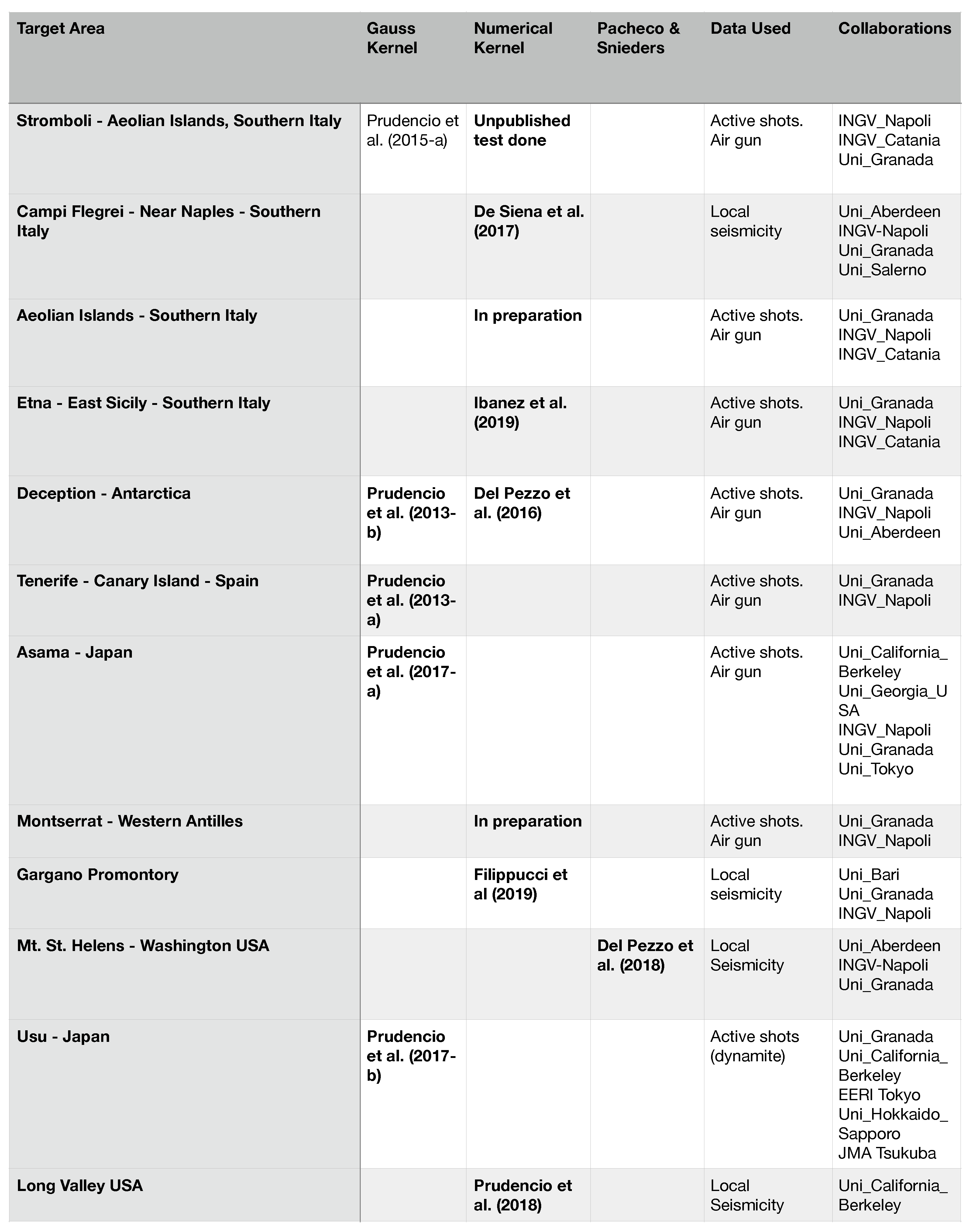
2.4. Application to Real Data to Estimate the Seismic Attributes

The application of the above scattering models to the observations is done estimating the fit of the SEE to the model, in order to retrieve the attenuation parameters B 0 and L e 1 or their equivalents in Equation (3). In some recent attempts to obtain a separate estimate of intrinsic- and scattering-attenuation coefficients some researchers (see e.g., [20]) succeeded in the estimation of l * , the mean free path for Energy transport (see the previous definitions) in association with Q c , Q-coda, calculated for early coda. In reality, while Q c approaches the true Q i when estimated soon after the S-wave train (early coda), l * cannot be, in general, considered as a good estimate of l g ( l g = v Q s 2 π f ) . However, in the case of Diffusion regime, the two procedures (measure of the time delay between S-wave onset and maximum of SEE or the fit to the Diffusion model should yield the same results inside the uncertainties). We do not describe the details of this approach in the present Section. Imaging methods are almost necessarily based on a single station estimation of B 0 and L e 1 . A severe problem arises in the fit of ETM to the SEE, caused by a trade-off occurring when the two parameters, B 0 and L e 1 , are jointly estimated from the same seismogram. Fortunately, when shallow source events occur in very heterogeneous media (Diffusion regime), like for example the seismograms recorded in volcanoes from natural seismic events or from artificial events, an almost unbiased separate estimate of B 0 and L e 1 can be achieved ([21,22] and references therein). In all other cases (media with medium-to-low heterogeneity, seismograms recorded from deep natural sources), the trade-off problem prevents the possibility of obtaining separate estimates of B 0 and L e 1 . In these cases, the unique option is to use the asymptotic approximation of the model (SSM) to the data, inverting for L e 1 parameter. Looking at Equation (5), one could think to separately obtain the product B 0 L e 1 and L e 1 , knowing the effective source intensity W 0 . This is, in principle, possible when the single scattering regime effectively prevails (see e.g., [23]). In all the other cases, an improper model assumption (the single scattering regime does not prevail) introduces a severe bias.
It is important to remark here that the base assumption made until now on the nature of the scattered waves is that they are essentially Shear waves. This assumption is corroborated by many experimental observations from passive data (see [2] for a review on this subject) which all demonstrate that shear waves prevail inside the coda wave radiation. Moreover, due to the unfavorable S to P and largely advantageous P to S wave conversion in the scattering, the artificial events that are generated by explosions also show a coda wave train largely composed by shear waves. This last experimental evidence is based the possibility to use the artificial events seismic coda for the evaluation of the space attenuation pattern, as shown in this review paper.

2.5. The Time Evolution of Coda Waves Studies

Really interesting and instructive is the historical evolution of the studies on coda waves. Scientists trying to measure the attenuation parameter of a given area from coda waves, often for seismic risk purposes, initially (and then widely) applied the SSM to experimental coda envelopes from local earthquakes, generally measuring only Q c . In the pioneering works of [3,4,5], among many others, SSM was used to retrieve the space averaged attenuation parameter from local earthquakes, even in the cases of highly heterogeneous earth media, causing problems in the interpretation of the measured attenuation parameters. Due to the use of an inappropriate model, Q-coda cannot be considered in facts an unbiased estimate of the average total Q (being the single-scattering approximation far from being realistic in most cases). Despite this problem, Q-coda still remains a widely measured parameter (due to the mathematical simplicity of SSM) used to relatively compare different tectonically active zones each other, or, much more recently, to obtain coda-Q images in zones of tectonic interest (see e.g., [20]).
DM was instead successfully used to invert for separate attenuation parameters in volcanoes ([21,22] and references therein; [9]). The main results from these studies is the striking observation that scattering attenuation largely prevails on the intrinsic absorption in volcanoes.

3. The Heuristic Method to Calculate Sensitivity Kernels

3.1. Early Q-Coda Images

Once the first measures of seismic attenuation based on coda waves studies were experimentally obtained, researchers tried to interpret the different physical properties of the propagation medium in association with the tectonic regimes of the area under study. The main problem to solve for a correct interpretation of the experimental results was the association of the measured attenuation parameters with the earth volumes sampled by the coda radiation in order to add information to the structural, tectonics or geodinamic maps. Researchers formerly found that Q-coda is an indicator of the tectonic properties. Aki and Chouet [4] calculated Q-coda as a function of frequency, fitting SSM to SEE for data from different areas with peculiar tectonic characteristics, finding different frequency patterns in different tectonic domains. Dainty [24] found that Q-coda has a dependence on frequency of the type
Q c = q 0 ( f / f 0 ) n
where q 0 is Q-coda at the reference frequency, f 0 , and f is the central frequency of the frequency band where Q c has been estimated. A great number of successive papers implicitly chose f 0 = 1 Hz as reference and interpreted q 0 and n as parameters that are associated with the tectonic activity in a given region (see e.g., [25] and the references in [2]). Singh and Herrmann [26] measured a significant space variation of q 0 through United States of America and plotted a 2D image of q 0 (corresponding to Q c at the reference frequency of 1 Hz) for USA. The paper by [26] can be considered as the first (at our knowledge) attempt to obtain a 2D Q-coda image (space distribution). The successive (really very few) studies aimed at obtaining the space distribution of Q-coda anomalies in a given area, were carried out using the simple technique of assigning the single source-receiver Q-coda to a point in the space—generally the middle point between source and receiver—and eventually plotting the isolines of equal Q-coda in the map after a kriging process [26]. This procedure is simple but highly approximate, as the signals from scattered waves composing the coda seismogram are all generated (at different times) inside the ellipsoid (an ellipse in 2D) whose max axis length is proportional to the coda max lapse time considered. This ellipsoid is generally called “scattering volume”. The equation of its boundary in 3D is given by
x 2 ( v t l a p s e 2 ) 2 + y 2 ( v t l a p s e 2 ) 2 x d 2 + z 2 ( v t l a p s e 2 ) 2 x d 2 = 1
which in 2D (scattering ellipse) reduces to
x 2 ( v t l a p s e 2 ) 2 + y 2 ( v t l a p s e 2 ) 2 ( 2 x d ) 2 4 = 1
where the source is located at { x d , 0 } and the receiver at { x d , 0 } and t l a p s e is the maximum lapse time measured along the coda from the origin time (see e.g., [27]). An example is reported in Figure 2.
Xie and Mitchell [28] described a back-projection method based on Q-coda estimates calculated fitting data to the single-scattering model. These authors assumed that Q-coda was representative of the attenuation averaged inside the scattering ellipse, which, in their case, was implicitly assumed as a (very) simplified Sensitivity Kernel for Q-coda.

3.2. The Introduction of Peak Delay Time and the First Attempts to Separate Intrinsic from Scattering Q

More recently, [29] mapped Q c for Japan, finding a strict correlation of Q-coda anomalies with intrinsic-Q anomalies. Calvet et al. [30] used both Q-coda and peak delay measurements as observables for calculating the space distribution of attenuation in the Pyrenees. Even in these more recent papers, the space distribution of attenuation parameters deduced by the SEE is empirically calculated mostly in two dimensions, in the simplifying assumption that the measured parameters can be reasonably attributed to an ellipsoidal area or, simplifying, to a rectangular strip, covering source, and receiver, which should represent the area where most of the scattered waves come from.
However, the geometrical shape of this area (or volume in 3D) and the true space distribution of the scattering secondary sources should be more precisely calculated in order to avoid further (and sometimes unjustified by the physical point of view) approximations. Attenuation estimates derived from scattered waves should thus be associated with the corresponding scattering volume, and not with a single point or with a simple area inside it. Sensitivity Kernels for scattering mathematically represent this association, and their knowledge is thus necessary for Q-coda imaging. In particular, Sensitivity Kernels for scattering represent important means to spatially individuate the scattering time anomalies detected by coda-wave interferometry [15].
A deep and exhaustive review on the state of art on Sensitivity Kernels is reported in the Introduction of [14], in [15] and in the book of [11]. Here, we do not review neither the above cited theoretical studies nor the experimental results based on the theoretically derived Sensitivity Kernels, but we will focus the present paper on the calculation of the Sensitivity Kernels with an heuristic, but fast and easy, Monte Carlo-based method and on their use in coda wave imaging.

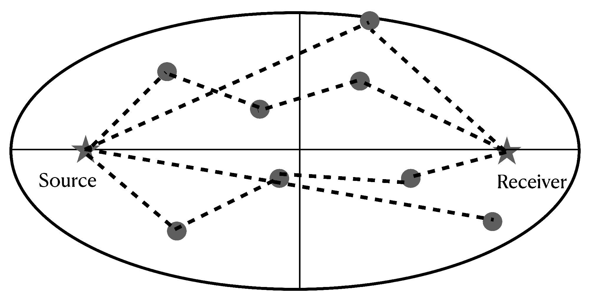
3.3. Sensitivity Kernels for Scattering Radiation

Sensitivity Kernels can be thought as the space functions describing the effective spatial sampling of the scattered waves. They permit to spatially confine the attenuation anomalies measured through coda waves, thus increasing the possibility to unveil heterogeneous Earth structures and interpret them in terms of rock quality. Their precise knowledge is essential for any attempt to obtain an attenuation image from coda waves.
Several studies have proposed physically grounded approaches to calculate these Kernels. Among these, Pacheco and Snieder [13] derived a 2D sensitivity function able to locate a scattering anomaly producing a sensible variation in the pattern of the SEE; Obermann et al. [12] based the estimation of the sensitivity function on the so called “locadiff” kernel introduced by [6,31], and further developed by [10,11] and more recently by [32]. Mayor et al. [14] calculated 2D Sensitivity Kernels for coda waves in the assumption of isotropic scattering and [15] in the case of 2D anisotropically scattering media, while [33] in the case of 3D single scattering. All the above papers adopted a theoretical approach in the framework of Radiative Transfer Theory or the Diffusion model, focusing their results at mapping the spatial changes in attenuation on the base of coda wave observations from distributed sources recorded at a seismic network. For all of the details, the reader may refer to the above cited papers and to the Appendix A4 of [16]. However, we remark that the heuristic approach discussed in the present review may represent a progress in direction of practical use of the imaging methods in non-homogeneous media, because the numerical simulation, differently from the above cited rigorous and physically grounded approaches, can be easily carried out in the heuristic approach, even in non uniform media.

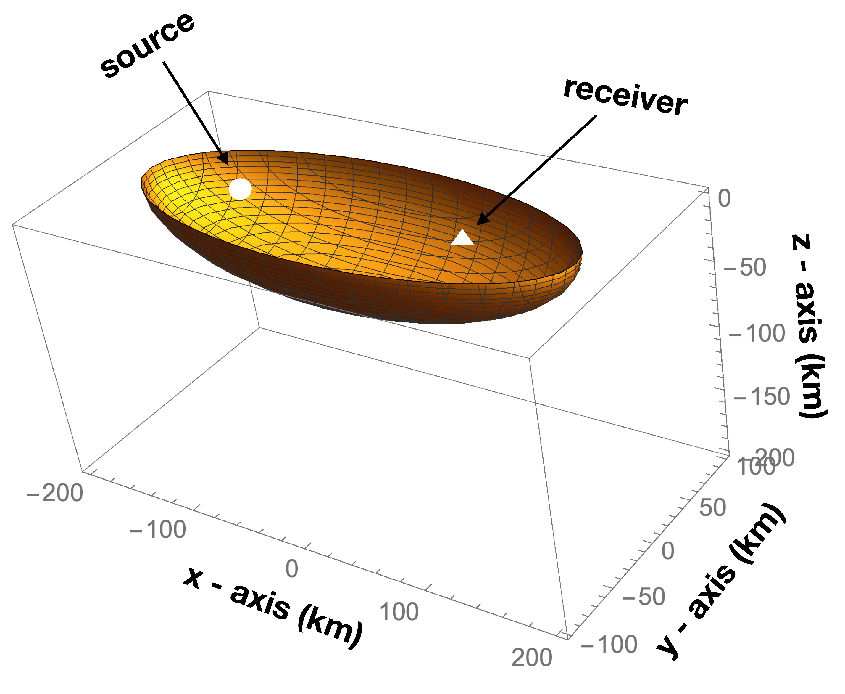
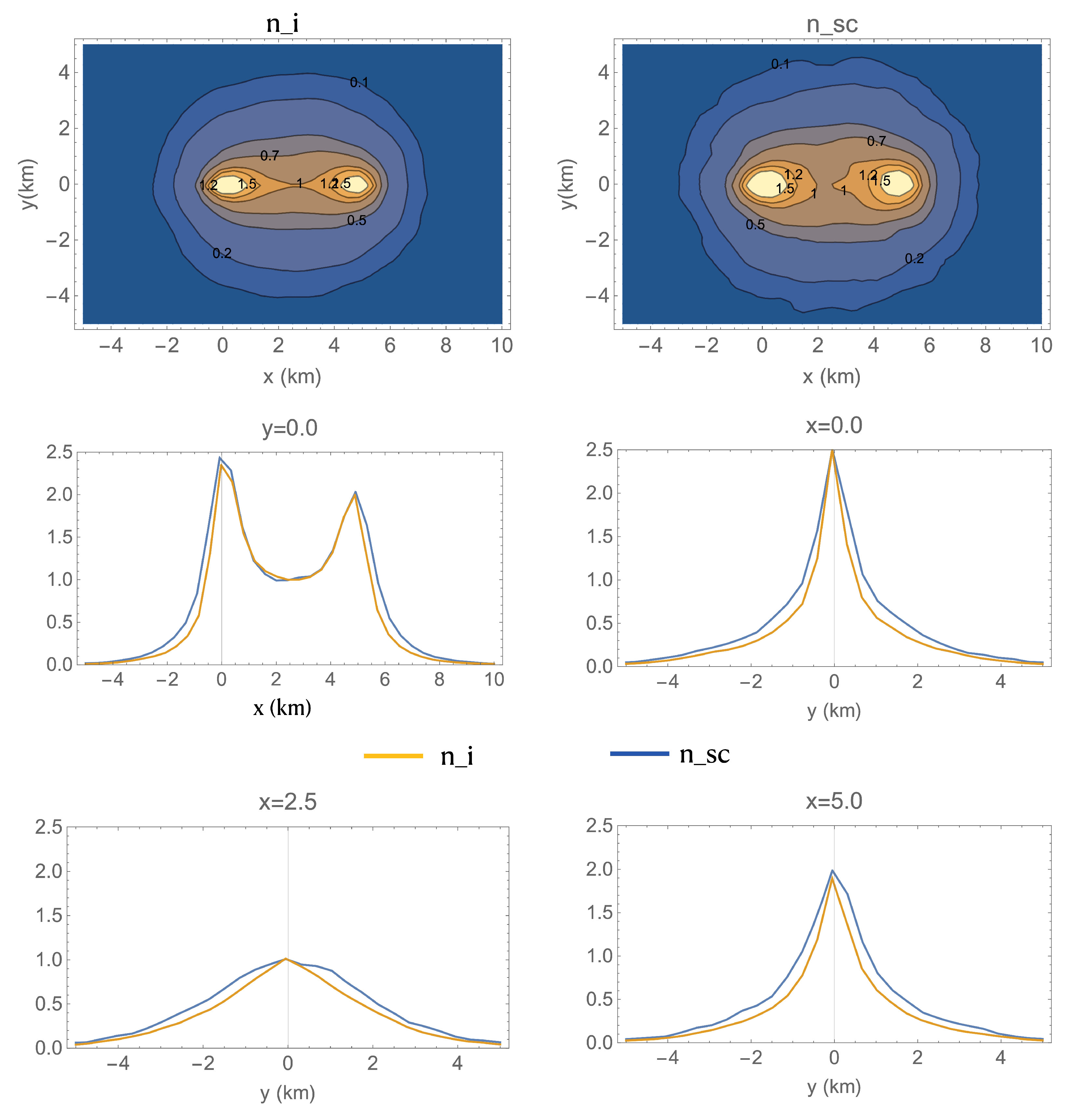
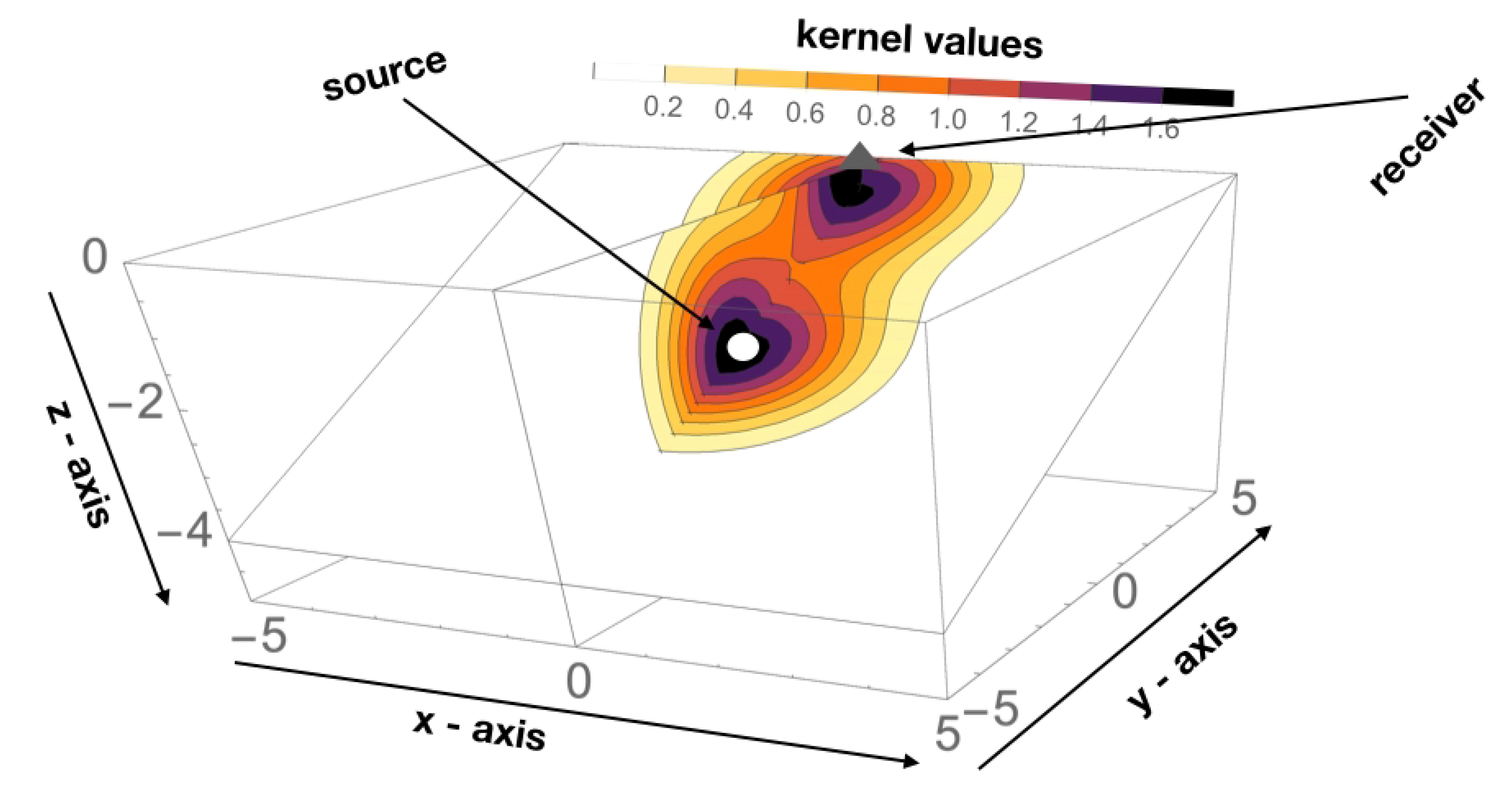
3.4. Numerical Simulation to Estimate the Sensitivity Kernels for Coda Waves

Theoretical approaches to calculate the Sensitivity Kernels in 2D and 3D have been adopted in the assumption of constant velocity in a half space. To take into account realistic velocity models (with velocity increasing vs depth together with the presence of velocity discontinuities), numerical simulations are necessary. We use a Montecarlo approach to solve the transport equation following the scheme of [34]. In this approach, the total seismic energy is simulated splitting the Source Energy, E 0 in a number, N, of energy “particles” of unit energy u, so that E 0 = N u . Each particle is emitted with a uniformly distributed random angle from the source. When a single particle encounters a scatterer, it changes direction randomly in the interval 0 2 π (isotropic scattering). The probability that a particle of unit energy encounters a scatterer is given by 1 E x p [ η s v t ] η s v t (Yoshimoto, 2000) where η s is given by Equation (3); at the travel time t, a fraction of its energy, 1 E x p [ η i v t ] , is absorbed by the propagation medium and transformed into heat, while collisions are assumed as purely elastic, with no Energy damping. After a random number of collisions, the particle reaches the receiver at a given lapse time, measured from the origin time, t l a p s e . The energy time envelope is finally obtained by the time histogram of all the particles arriving at the receiver, corrected for the quantity E x p [ η i v t l a p s e ] .Thus, the value of the energy envelope (at a given lapse time) is the sum of the energies carried out by the particles at the end of all the scattering process, altogether arriving in a small time interval around t. The details of this procedure are reported in [34]. A sketch of the simulation is shown in Figure 3.
The energy particles forming the Energy envelope sample a portion of the propagation medium associated with the attenuation parameters assumed in the simulation. Thus, we can heuristically assume that the volume elements (in which the whole medium is divided) crossed by more particles weight more in forming the energy envelope of each seismogram. Counting the number of times a particle crosses a volume element and the number of collisions inside the same element, we can calculate these weights for all of the propagation volume.
Thus, the weighting functions are thus determined in the following steps. (1) The Energy envelope is generated, assuming a propagation medium marked by three parameters: the half space velocity, v, (or the velocity depth pattern, v [ z ] ) , the scattering attenuation coefficient, η s , and the intrinsic attenuation coefficient, η i . The computation is stopped at a given lapse time: t l a p s e . (2) During the propagation, the position of the Energy particle and the position where the collisions occur are stored in two separate memory registers. (3) At the end of simulation, the spatial density of collisions, n s c ( x , y , z , x r , y r , x s , y s , z s ) and the path density, n i ( x , y , z , x r , y r , x s , y s , z s ) are calculated in a volumetric cell Δ V = Δ x Δ y Δ z , , where Δ x , Δ y , Δ z are small spatial coordinate intervals. The quantities n s c and n i are proportional, respectively, to the probability that the volumetric cell centered at { x , y , z } affects the Energy Envelope formation. The general spatial pattern of n s c and n i thus depicts the contribution of each cell to the coda formation. n i and n s c can be thus considered as Sensitivity Kernels, respectively, for intrinsic dissipation and scattering attenuation, to be used for imaging purposes. It is important to remark that n i and n s c depend on space, source, and receiver position and on v , η i , η s , and t l a p s e , despite these last are dropped out for simplicity. An example of their two-dimensional plot is shown in Figure 4. Hereafter, we will call them Space Weighting Functions (SWF).
The example shown in Figure 4 represents typical patterns in a very inhomogeneous earth medium, like that characterizing a volcano.

4. Analytical Approximation of the Space Weighting Functions

The two numerically calculated Space Weighting Functions n i ( x , y , z , x r , y r , x s , y s , z s ) and n s c ( x , y , z , x r , y r , x s , y s , z s ) , experimentally result similar to each other for a wide set of { η i , η s } couples, corresponding to values of quality factors (both intrinsic and scattering) smaller than 300–400 and short (less than 30 s) t l a p s e . Assuming a constant wave speed in this range of values, we can thus approximate both n i ( x , y , z , x r , y r , x s , y s , z s ) and n s c ( x , y , z , x r , y r , x s , y s , z s ) by a single analytical function, n ( x , y , z , x r , y r , x s , y s , z s ) . In different assumptions, this simplification is not possible, and a numerical simulation of SWF becomes necessary for each source receiver couple.
We adopted the following method to find the analytical approximation of n ( x , y , z , x r , y r , x s , y s , z s ) , valid in the range of values above described.
(1) The Space Weighting Functions are first calculated in two dimensions, while using the Monte Carlo method for a wide set of feasible parameters and distances, setting the source at the origin and receiver at a point on the horizontal axis, at a distance D = ( x s x r ) 2 + ( y s y r ) 2 + z s 2 from the source. The shape of the weighting functions result to be insensitive to η i , and depending on η s , D and t l a p s e . We first set t l a p s e = 15 s, a value that is characteristic of the duration of the small energy artificial events fired in the sea nearby some volcanoes for Tomography purposes.
(2) We calculated a suite of weighting functions, assuming that the quantity D spans from 5 to 20 km and η s from 0.8 to 0.04, which are typical values measured in volcanoes [2]. The calculations were carried out using 3 × 10 5 energy particles and a half-space constant velocity, v = 2.0 km s 1 .
(3) We used a trial and error approach for finding the analytical expression of a function that fits well the pattern shape of the numerical weighting functions. These last were normalized at their value at the middle point between source and receiver.
(4) The function
K n u m 2 D ( x , y , x r , y r , x s , y s ) = 1 6 π ( D δ ) 2 e x p x x r + x s 2 2 2 δ D 2 + y y r + y s 2 2 2 δ D 2 + 1 2 π ( δ D ) 2 e x p x x s 2 2 δ D 2 + y y s 2 2 δ D 2 + 1 2 π ( δ D ) 2 e x p x x r 2 2 δ D 2 + y y r 2 2 δ D 2
visually fits the gross features of the numerical weighting function, in a wide interval of D values. δ represents the spatial aperture of the weighting function in 2D. We trial and error found that δ = 0.2 is the best choice in the interval 1 < D < 60 even tough the numerically evaluated weighting function shows a sharper pattern around source and receiver coordinates. However, it is worth saying that the use of Equation (16) in the imaging procedure (see later in this paper) instead of its numerical counterpart produces almost similar images. For a wider discussion about this point see [16]. In the Figure 2 of the paper of [16], the comparison between the numerical result and the analytical function (1) is shown as an example. The use of this approximation greatly reduces the computer time, avoiding the numerical synthesis of n s c for each source-receiver couple available in the data set.
(5) Being the velocity, v , constant (half-space approximation), Equation (16) can be easily extended to 3D upon consideration of symmetry around the segment connecting source to receiver. Here, we report the 3D extension of Equation (16)
K n u m 3 D ( x , y , z , x r , y r , x s , y s ) = 1 6 π ( δ D ) 3 e x p x x r + x s 2 2 2 δ D 2 + y y r + y s 2 2 2 δ D 2 + z z r + z s 2 2 2 δ D 2 + 1 2 π ( δ D ) 3 e x p x x s 2 2 δ D 2 + y y s 2 2 δ D 2 + ( z z s ) 2 2 δ D 2 + 1 2 π ( δ D ) 3 e x p x x r 2 2 δ D 2 + y y r 2 2 δ D 2 + z 2 2 δ D 2
In Figure 5 and Figure 6 are shown, respectively, examples in 2D and one example in 3D.

5. Sensitivity Kernel for Q-Coda

In the case of buried sources (or natural earthquakes with depth comparable with epicentral distance), the assumptions made in calculating the approximation of SWF given by Equation (17) are invalid. This is due to the the strong heterogeneity present in the shallowest layers and disappearing in the deepest layers, where the diffusion regime does not still strictly hold. In this case, a multiple scattering model fit SEE better than a diffusion model. However, fitting Equation (4) to the experimental energy envelopes, the single path separate estimate of B 0 and L e 1 results, as already discussed, affected by a severe trade-off between the two parameters.
The only possibility is to fit the envelope data to a simpler and approximate equation, which avoids the coupling of of B 0 and L e 1 in the fit, strongly reducing the trade-off. A simple way to overcome the problem is to estimate L e 1 and B 0 from the fit of SEE (normalized for the source intensity) to the first order approximation of the ETM model Equation (5) reported by [2] and successively by [17], which is here rewritten to facilitate the readers:
E s s ( r , t , B 0 , L e 1 , v ) = W 0 δ ( t r / v ) 4 π v r 2 e x p ( r L e 1 ) + W 0 H ( t r / v ) B 0 L e 1 4 π r v t L n ( 1 + r / v t 1 r / v t ) e x p ( v t L e 1 )
Fitting this equation to SEE after excluding a time interval around the direct arrival, severe trade-off problems between B 0 and L e 1 disappear, as one could estimate L e 1 from the slope of the Log Energy Envelope while the product B 0 L e 1 from the Envelope level at the origin. It is noteworthy that Equation (18) is equivalent to the single-scattering model developed by [5] (excluding the source term). It becomes valid in the case of media with low heterogeneity and short lapse times. In such a case L e 1 , being η s small, is controlled by intrinsic attenuation (see Equation (3)). However, when Equation (18) is fit to SEE recorded in media with high heterogeneity, the physical meaning of the retrieved parameters B 0 and L e 1 becomes controversial, being the fitting function based on improper assumptions. It is anyway worth reminding that L e 1 = 2 π f v Q c o d a 1 , Q c o d a being the coda quality factor [5] often used to compare areas with different attenuation properties [30]. Therefore, in principle, L e 1 (or Q c o d a ) space distribution can be used to depict an attenuation image once that the corresponding SWF that may be called K c o d a , can be calculated. Taking Q c o d a formerly into account the total attenuation, SWF should weight the sum of energy lost by scattering and intrinsic dissipation.
It is worth remembering that, in practice for most experimental data, Q c o d a is far from being an unbiased estimate of total-Q. This parameter results much closer to Q i , the intrinsic-Q, than to Q T , the total-Q, in media with medium-low heterogeneity. In other words, Q c o d a tends to Q i for increasing Q s . This essentially depends on the use of the single scattering approximation of Paasschen’s solution for the Energy Transport Equation in the data fitting, which, on the other hand, became necessary to avoid the trade off in the parameter estimates. Q c o d a can be thus defined as an hybrid parameter, valid to discriminate between different attenuation regimes, but unable to reach a correct interpretation on which type of attenuation mechanism prevails (see e.g., [35]).
To show how severe is the bias introduced in using the First Order Approximation of ETM when fit to the data, we have fit the First Order Approximation of ETM (in practice, the single-scattering model) to Equation (4) calculated for different couples of Q i and Q s , truncated at short (30 s) lapse time. The results are shown in Figure 7, where the contour plot of Q-coda as a function of Q i 1 and Q s 1 is shown. For earth media characterized by an intermediate heterogeneity (left panel), Q c o d a 1 is practically independent of Q s 1 and similar to Q i 1 . Differently (right panel) Q c o d a depends on both Q i and Q s
K c o d a can be approximated by Equations (16) and (17), respectively, in 2D and 3D. To avoid the approximation done in Equations (16) and (17), a possibility could be the procedure that was described by [13]:
K c o d a ( ρ , T , B 0 , L e 1 , v ) = 0 t l a p s e E ( r s ϱ , τ , B 0 , L e 1 , v ) E ( r ϱ r , T τ , B 0 , L e 1 , v ) d τ E ( r s ϱ , t l a p s e , B 0 , L e 1 , v )
where ϱ is the space point with coordinates { x , y , z } , t l a p s e is the maximum lapse time, τ is the integration variable (dimensionally a time). The integral can be numerically calculated, as shown in the Appendix of [36].
In Figure 8, we reproduce the SWF calculated using both Equations (19) and (16) in the case of a shallow source at distance of 10 km from receiver, for a lapse time of 50 s, B 0 = 0.5 , L e 1 = 0.01 , and a half space velocity, v = 3.0 km/s. The patterns are quite similar, both showing maxima at the source and receiver positions. The SWF are both normalized at their value in the middle of the source-receiver segment.
To give a short summary of the practical criteria of application of the SWF previously discussed, we refer to the scheme of Figure 9. In this scheme, we show that for increasing heterogeneity and shallow sources (surface propagation), diffusion regime is appropriate. In this case it is simpler to estimate the 2D or 3D polynomial approximation of numerically calculated SWF. In the case of any other regime (low or intermediate heterogeneity, source depths not superficial), as already said, there is a trade off between the two parameters B 0 and L e 1 when jointly estimated by the fit of ETM to the single Energy Envelope. In this case one could more simply estimate the approximate parameter Q c o d a and use one of the SWF that is shown in Figure 8 to image the effective Q i space pattern.

6. Imaging Methods Based on SWF

This method is based on measuring, for each receiver-source pair, the seismic attributes given by the couple ( B 0 , L e 1 ) or the correspondent couple { Q i , Q s } or the single parameter Q c . In the scientific literature, well sounded methods describing how to obtain such estimates by fitting data with models are available (see e.g., [2]). However, we remark that separate single source-receiver couple estimates of Q i and Q s can only be obtained in strongly heterogeneous earth media (diffusive earth media, like volcanoes, [21]). This is possibility due to the particular shape of seismogram envelopes in such media, characterized by a maximum that does not coincide with the S-wave direct arrival, but it is late with respect to this arrival by a time delay (of several seconds), depending only on the amount of scattering and not on the intrinsic dissipation. The fit to the diffusion model is thus well constrained by this time delay, allowing for an almost unbiased estimate of separate Q i 1 and Q s 1 . In a seismogram of a local low-magnitude earthquake that occurred in a non-diffusive earth medium, the time delay between the S-wave onset and the time corresponding to the Envelope maximum is not proportional to the scattering mean free path, l g , but to l * , the transport mean free path. The two quantities are different, the difference becoming smaller when heterogeneity increases. In practice, except some cases (see e.g., [37]), it is possible to only measure Q c that is formally a combination of intrinsic and scattering attenuation from the Envelope shape. To give a very simple rule, when diffusion model is a reasonable approximation of the geological reality, a separate estimate of intrinsic and scattering attenuation coefficient at a single source-receiver couple is possible (for shallow sources). For all other cases, the separation is almost impossible and the only measurable (unbiased) parameter is Q c .
Hereafter we will denote with K n u m (stands for “Numerically calculated Kernel”) the generic Space Weighting Function. The suffix 3 D (conversely 2 D ) indicated the space dimensions and index k the single source receiver couple for which the SWF is calculated. K n u m in other words can represent the scattering-, the intrinsic- or the coda-Q Sensitivity Kernel.

6.1. Imaging Methods Based on SWF’s in Diffusive Media

In Section 4, we stated that, for values of quality factors (both intrinsic and scattering) smaller than 300–400 and short (less than 20 s) lapse times the two numerical functions n s c and n i have a similar form and can be usefully approximated by the Equation (17) or by Equation (16) in 2D. The above range of values ( Q i < 400 ; Q s < 400 ) corresponds to highly heterogeneous media (see also the scheme of Figure 1). In such media, diffusion approximation of Equation (6) is appropriate ([22,38]). One of the possible methods to fit the SEE to the Diffusion Equation (6) to retrieve simultaneously the couple { Q i , Q s } (or the corresponding parameters: see Equation (3)) is described in [21].

6.2. The Projection Method

In the Projection Method, the value of the attenuation parameters couple, Q i 1 and Q s 1 (or the corresponding parameters: see equations 3), estimated for a single source-receiver couple, is assigned to the whole space volume, weighted by the SWF associated to the same source-receiver couple, K n u m 3 D (or its equivalent in 2D). Discretizing the the study area or volume in cells, for each cell a number, N, of weighted measures will be thus available, where N is the number of source-receiver couples. However, for many cells, the value of the SWF will be extremely small. Finally, the best estimator for the value of { Q i 1 , Q s 1 } is calculated in the assumption of Gaussian statistics (the weighted arithmetical average):
Q 1 ( x , y , z ) = k = 1 N K n u m k 3 D ( x , y , z , x r k , y r k , x s k , y s k ) Q k 1 k = 1 N K n u m k 3 D ( x , y , z , x r k , y r k , x s k , y s k )
where Q 1 ( x , y , z ) is the estimate in the space point { x , y , z } (center cell), k is the source-receiver index spanning from 1 to N, Q k 1 is the k t h estimate (we drop out the indexes i or s for simplicity, being the K n u m the same for both intrinsic and scattering attenuation) and K n u m k is the k-th SWF. { x r k , y r k } and { x s k , y s k } are, respectively, the coordinates of receiver and source for the k-th source-receicer couple.

6.3. The Inversion Method

The Inversion Method assumes that Q k 1 can be written as the space weighted average of the set of the true values, characteristic of each volume cell:
Q k 1 = c e l l s K n u m k 3 D ( x , y , z , x r k , y r k , x s k , y s k ) Q 1 ( x , y , z ) c e l l s K n u m k 3 D ( x , y , z , x r k , y r k , x s k , y s k )
where Q 1 ( x , y , z ) are the unknowns and {x,y,z} represents the space position of the single cell. The linear system of N equations can be solved with an optimization procedure (Linear Least Squares, or SVD). We remain that Q k 1 represents indifferently Q i n t r i n s i c or Q s c a t t e r i n g and that n s c and n i are a good approximation of K n u m k 3 D . n s c and n i are actually similar for a wide set of { Q i 1 , Q s 1 } couples (see above in Section 4).

6.4. Equivalency of the Two Approaches

We would like to remark that the two imaging methods described in Section 6.2 and Section 6.3 are, in principle, not equivalent, but it can be demonstrated (see e.g., [39]) that the two approaches tend to give the same result for large values of N. It is also worth to say that the term “Projection” associated with the method of Section 6.2 may be misinterpreted: it is not a formal Back-Projection method, as described i.e. by [40], where Back-Projection is described as one of the methods apt to solve an inverse problem. It can be seen instead as a generalization of the simple procedure of assigning a single estimate of Q i 1 or Q s 1 to a point (or to a volume) in the space. In this generalization, the single estimate of Q i 1 or Q s 1 is assigned to each space point, this last being however weighted for the correspondent SWF.

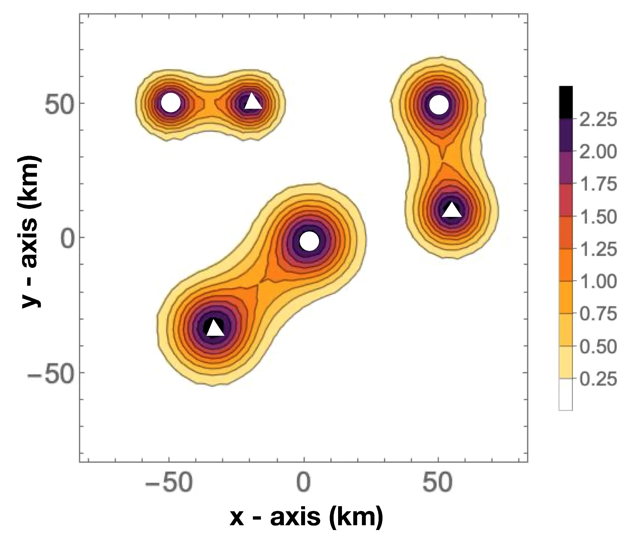
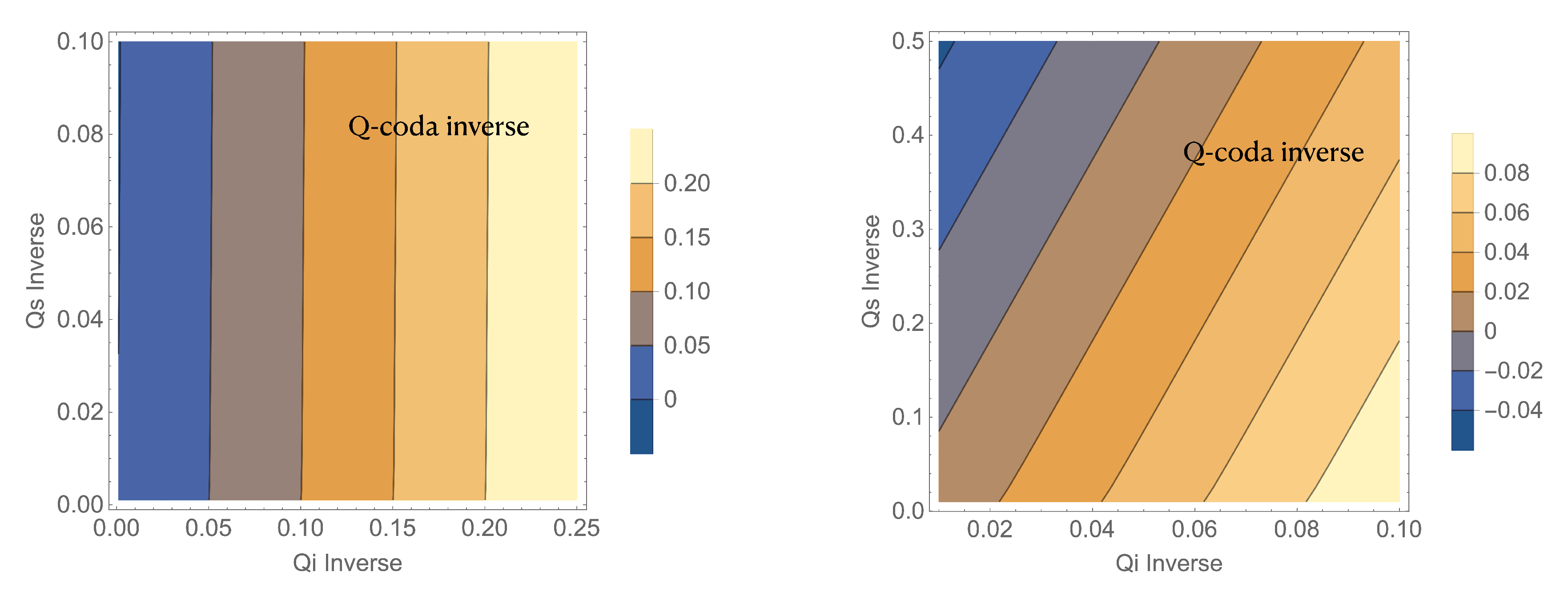
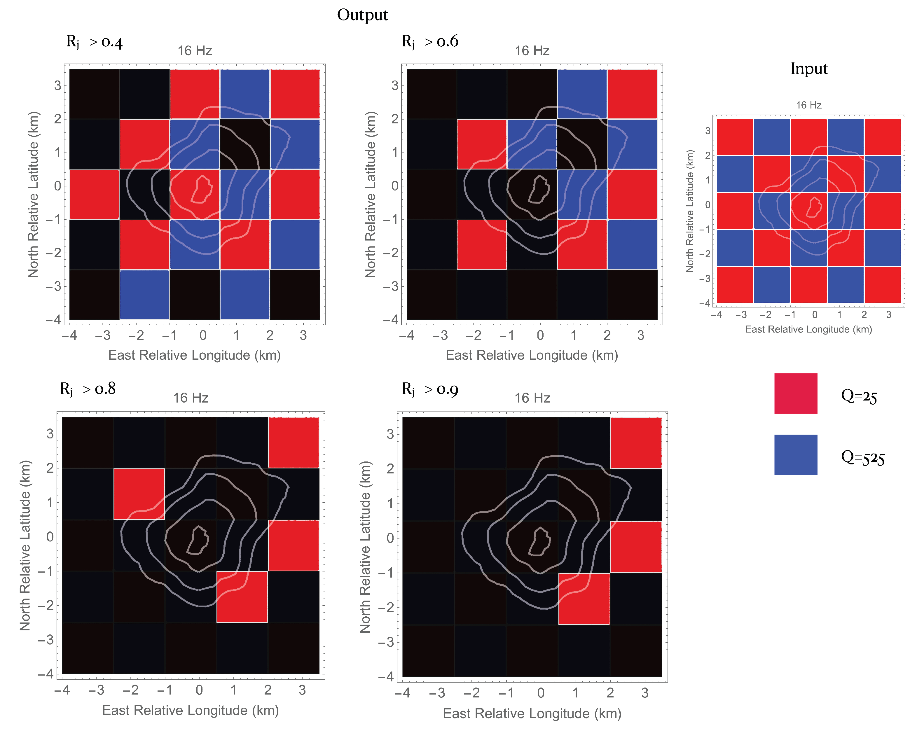
6.5. Sensitivity Tests

Usually, sensitivity tests check capability and accuracy of the obtained results. They are carried out: (a) solving the forward problem for a pre-determined input, (b) using the results thus obtained as input for the method utilized, and (c) comparing results with input. This approach is possible for the Inversion method using as forward model Equation (21), while it is formally impossible for the Projection method, which is not based on any forward model. In this last case, we empirically define a “Resolution” function that assigns to the space cells a weight proportional to the probability that results in the cell approach the true values. Alternatively, we can use an hybrid approach as a sensitivity test for the Projection method: starting from a given input (for example, a checkerboard structure with alternatively high and low attenuation parameters) we can use Equation (21) as forward model and use Projection method to compare input and output. The shortcomings are that (1) the empirical “Resolution” function, as it will be specified in the next sub-Section, does not give information on the effective resolution (how the input checkerboard cells are effectively resolved), while (2) the hybrid method is based on an “assumed” forward model.

6.6. The “Resolution” Function for the Projection Method

The weighting functions K n u m 3 D ( x , y , z , x r k , y r k , x s k , y s k ) or the 2D correspondent K n u m 2 D , represent the probability that, for the k-th source-receiver couple with coordinates, respectively, { x s k , y s k } and { x r k , y r k }, the estimated parameter couple ( Q k i 1 and Q k s 1 ) is effectively the true value at the space point with coordinates x, y and z. We remain that in highly heterogeneous media the weighting functions are practically equal for Q i 1 and Q s 1 ; therefore, the test is carried out for a generic Q 1 .
In order to simplify the equations, we slightly modify the notations with no substantial changes in the above equations.
  • The weighting functions (each normalized for their maximum) are represented by the quantities w i j where i is the event-source index and j represents the j- t h pixel of generic coordinates { x , y } . i spans from 1 to N where N is the number of source-receiver couples in the data set. j spans from 1 to M where M is the number of pixels (square regions in which the input image is divided).
  • q i j ¯ is the j- t h Q-value (or its inverse) measured for the i- t h source-receiver couple
  • q j is the output of the method for the j- t h pixel.
The “back-projection” method (using this notation) yields
q j = i q i j ¯ w i j i w i j
We remain that w i j represents thus the un-normalized probability that the actual i- t h measure, q i j ¯ , can be associated with the j- t h pixel.
Let us assume that the standard deviation, σ , is the same for all of the measures q i j ¯ . Applying the error propagation equation to Equation (22), we obtain
σ q j 2 = σ 2 i q j q i j ¯ 2
Because q j q i j ¯ = w i j i w i j , then it results that
σ q j 2 = σ 2 i w i j i w i j 2 = σ 2 ( i w i j ) 2 i w i j 2
As can be immediately seen, for the quantities w i j all equal to 1, σ q j = 1 N , as in a ordinary un-weighted average. Thus, it is natural to assume that the quantity proportional to standard error inverse (normalized by σ ) , σ / σ q j , represents an estimate of the resolution of the method. In other words, the cells showing smaller resolution should be associated with higher errors and vice-versa.
The Resolution at the j- t h pixel is thus given by
R j = ( i w i j ) 2 i w i j 2

7. Application to Real Data

7.1. Projection Method in the Diffusion Assumption

Several volcanoes have been studied with the aim of obtaining seismic velocity tomography images of their inner structures, mostly using active data (fired shots surrounding the target area). The complete waveform recorded at receivers located inside or around volcanoes are also a perfect input for the above described Projection (or Inversion) methods, being generated at surface in very heterogeneous geological environments. Untill now several applications of the Projection method have been carried out in 2 dimensions, using the approximate SWF described in the present paper. A comparison of results achieved using other kinds of SWF (of Gaussian Form, mainly) with those obtained using the SWF discussed in the present paper guarantees that in a first approximation the images are similar in the two cases. However, the small differences between the images achieved using SWF of Gaussian Form and the present one have never been investigated quantitatively. The reader can thus refer to the references of [16] and to the scheme of Figure 10 for an almost complete view of these results. We do not report here the images published in the papers referenced in the scheme, in order to avoid a too much heavy text, being this review focused mainly onto the methods. Detailed interpretations for every single volcano based on the images cited above can be found in the relative papers. It is however interesting to note that images of Stromboli (Southern Italy), Tenerife Deception Island (Antarctica), Asama (Japan), and Montserrat (Antilles - paper in press) show common interesting patterns which, in extreme synthesis, are: (1) the images of intrinsic attenuation are different from those of scattering attenuation; (2) the geological structures of the area, when they are known by independent geological studies, result to be generally well correlated with the pattern of the scattering attenuation contrasts. (3) the velocity anomalies are generally anti-correlated with the intrinsic attenuation anomalies. The above reviewed methods prove thus to be promising and useful, adding constraints to the interpretation of the velocity tomography images.

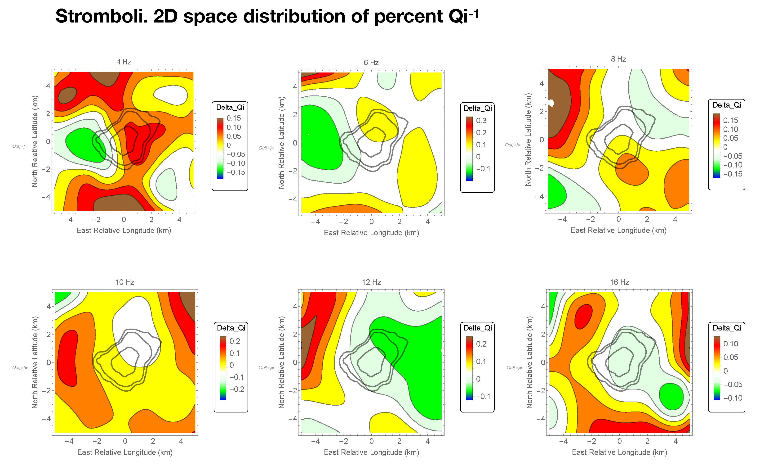
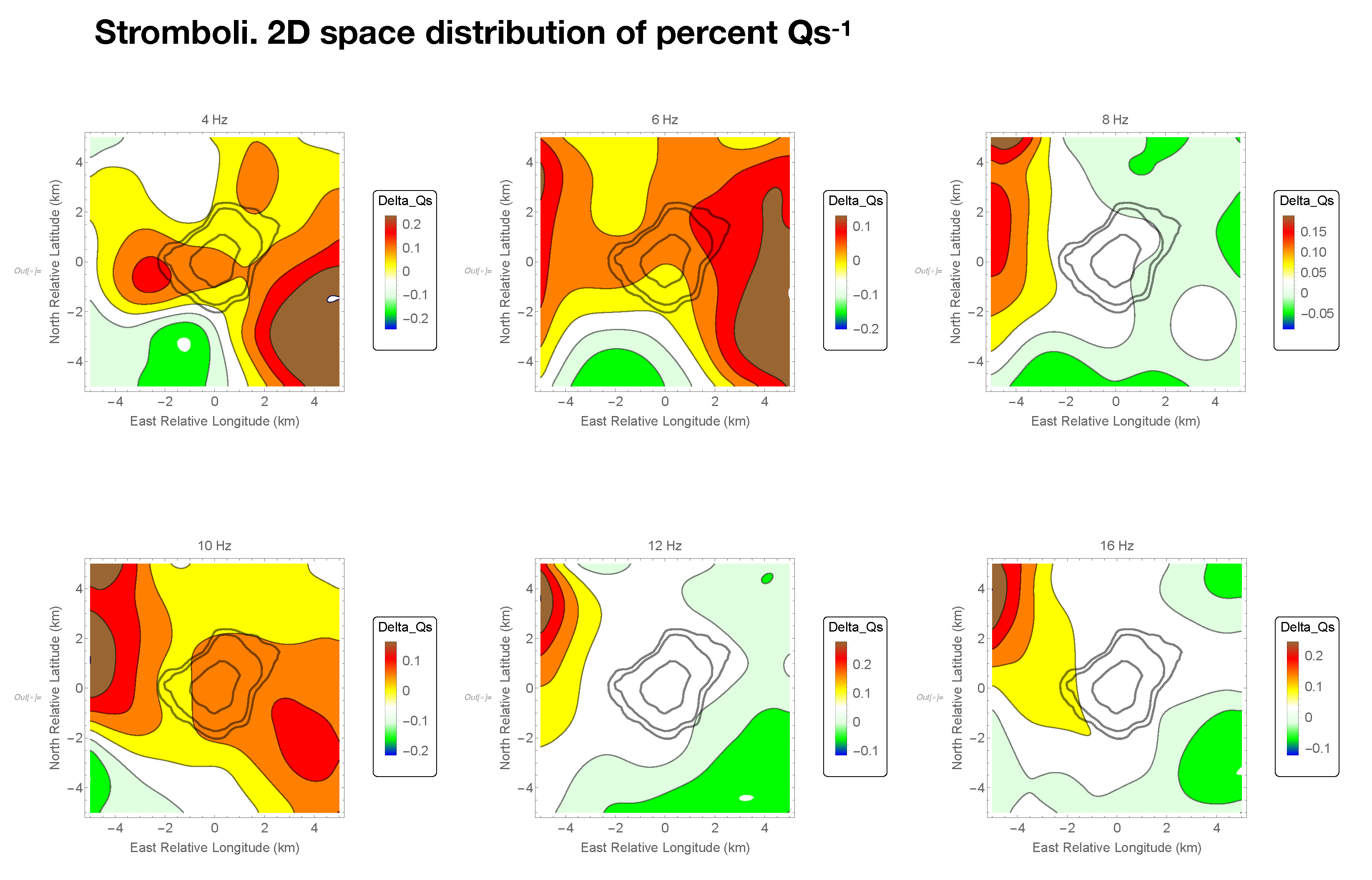
7.2. Projection Method Applied to Stromboli Volcano: A Revision of the Results

In the present paper, we show an application example of the 2D Projection Method to real data recorded at Stromboli volcano during an active (air gun) seismic survey carried out for velocity tomography purpose in November–December 2006 at Stromboli Volcano and surrounding areas [41]. More than 1500 offshore shots (see Figure 1 of [42]) were recorded by 33 in-land three-component receivers and by 10 OBS (ocean bottom seismometers), providing a data set composed of 21,953 waveforms. Original data used in the present work are the same of that used by [42], but in the present example we used a much more severe selection criterium: after a selection of the seismograms showing a signal to noise ratio at the end of coda signal higher than 2, we fit the SEE to equation (6). Subsequently, we further excluded all the data that showed an insufficient correlation coefficient in the fit and/or an attenuation parameter external to the interval 2.5–1000.
The results are shown in Figure 11 and Figure 12, where the 2D images of the Q 1 fluctuations with respect to the average are shown in the frequency bands centered at 4, 6, 8, 10, 12, and 16 Hz.
The resolution of the images shown in Figure 11 and Figure 12 is given by the space representation of Equation (25), as reported in Figure 13. In this figure, we show the resolution for a synthetic checkerboard-like input of alternate relatively high attenuation ( Q = 25 ) and low attenuation ( Q = 525 ) . Resolution is represented by a grey color grid overimposed to the checkerboard structure, with opacity inversely proportional to the Resolution. In this way, the original colors (represented aside the Figure at the right) are darkened when the sensitivity is low. From the same Figure, it is quite clear that there is a cell that is completely obscure in the North-Eastern sector of the Island (coast and main altitude isolines superimposed). Moreover, the Westernmost and Southernmost cells show a very low resolution.
.

7.3. Inversion Method in the Single Scattering Approximation

The Inversion method has been applied to Mt. St. Helens [20] and Campi Flegrei [43]. At Mt. St. Helens data allowed the extension of the method to the third dimension (depth) while at Campi Flegrei, being seismicity extremely shallow, the images show 2D lateral variations. In both zones, being the earth medium far from being described by a diffusion model, the separation between intrinsic- and scattering-attenuation was impossible. Q-coda was thus the estimated parameter. Interpretation, in this case, results in being more difficult, as one cannot directly attribute an attenuation anomaly to an increase/decrease of the earth heterogeneity or to a intrinsic attenuation anomaly. Despite this difficulty, the obtained results have helped in mapping debris flow, feeding paths and tectonic features of Mt. St. Helens, and in constraining the location of the magma source that is responsible of the pronounced ground uplift phenomena characteristic for Campi Flegrei area.

8. Conclusions

In the present review, we have discussed the methods based on coda wave imaging associated with the use of the numerically estimated SWF. The present SWF assumes an heuristic meaning, describing, cell by cell, the probability that the scattering phenomena are generated inside each pixel. In addition, this Kernel describes in the same way the probability that intrinsic dissipation has occurred in any pixel. Differences between scattering and intrinsic attenuation SWF may occur in media characterized by a sparse scatterers distribution, leading to many pixels being crossed by radiation with no or poor scattering phenomena inside.
Despite in literature the images are mostly bi-dimensional, they always result as an interesting complement to the ordinary velocity and direct (total) attenuation tomography images. Zones that are characterized by high total attenuation could actually be interpreted as highly fractured (when scattering attenuation prevails over intrinsic absorption) or as marked by the presence of fluids (as magma patches, when intrinsic absorption prevails over scattering attenuation). Moreover, the association of velocity and (separated) attenuation images may greatly help the interpretation, as fluid filled rocks are characterized by high Vp/Vs ratios. We would briefly summarize a scheme of applicability of the Sensitivity Kernels for scattering described in the the present review. Dealing with highly heterogeneous target zones (volcanoes) investigated using active shallow sources (as the case of Stromboli, described in a previous Section of the present review), the assumption of a Diffusion regime may be appropriate. In this case, a separate estimate of B 0 and L e 1 or of the correspondent quantities in Equation (3) is possible and two separate images of intrinsic- and scattering-attenuation can be obtained. In all other cases, being strongly biased the single path estimation of intrinsic- and scattering-attenuation, due to the trade-off between these two parameters [44] it is recommendable the use of Q-coda Kernels to obtain a Q-coda image of the region under study. To conclude, the pros in the utilization of these methods is that it is, in principle, possible to obtain separate intrinsic- and scattering-attenuation images, at least in the cases where earth heterogeneity is very high (and consequently a diffusion models holds well). Thus, volcanoes become the perfect candidates for the application of Sensitivity Kernels for coda waves to attenuation imaging.

Author Contributions

Conceptualization, E.D.P. and J.M.I.; software, E.D.P.; validation, E.D.P.; writing—original draft preparation, E.D.P. and J.M.I.; editing, E.D.P. and J.M.I.; Both authors have read and agreed to the published version of the manuscript. All authors have read and agreed to the published version of the manuscript.

Funding

This research received no external funding.

Acknowledgments

Researches reviewed were partly carried out under Grants No. PID2019-106260GB-I00.

Conflicts of Interest

The authors declare no conflict of interest.

Abbreviations

SymbolExplanation
NNumber of wave-particles in the simulation
η s Scattering coefficient. g = η s = 2 π f v Q s where f is the frequency
vWave speed
t l a p s e Lapse time (measured from origin)
η i Intrinsic attenuation coefficients. η i = 2 π f v Q i where f is the frequency
B 0 Seismic Albedo. B 0 = η s η i + η s
L e Extinction Length. L e 1 = η i + η s
n s c , n i Space density of scatterers and paths, respectively, or Space Weighting Functions
{ x s , y s } Source coordinates
{ x r , y r } Receiver coordinates
D ( x s x r ) 2 + ( y s y r ) 2 source-receiver distance
δ t time step used in simulations
Q i , Q s Intrinsic and Scattering Quality Factor
K n u m 3 D , K n u m 2 D Analytical expression of n s c , n i for high heterogeneity (diffusion)
EEnergy envelope
E d Energy envelope in the Diffusion approximation
E s s Energy envelope in case of Single scattering
q ¯ Measured Q-value
w i j The same of K n u m (to simplify notations)
R j Resolution function at j- t h pixel
AcronymExplanation
ETMEnergy Transport Model
DMDiffusion Model
SSMSingle Scattering Model
SEESeismogram Energy Envelope
SWFSpace Weighting Functions

References

  1. Obermann, A.; Planes, T.; Hadziioannou, C.; Campillo, M. Lapse time dependent coda wave depth sensitivity to local velocity perturbations in 3-D heterogeneous elastic media. Geophys. J. Int. 2016, 207, 59–66. [Google Scholar] [CrossRef] [Green Version]
  2. Sato, H.; Fehler, M.; Maeda, T. Seismic Wave Propagation and Scattering in the Heterogeneous Earth, 2nd ed.; Springer: Berlin/Heidelberg, Germany, 2012. [Google Scholar]
  3. Aki, K. Analysis of the Seismic Coda of Local Earthquakes as Scattered Waves. J. Geophys. Res. Solid Earth 1969, 74, 615–631. [Google Scholar] [CrossRef]
  4. Aki, K.; Chouet, B. Origin of coda waves: Source, attenuation, and scattering effects. J. Geophys. Res. Solid Earth 1975, 80, 3322–3342. [Google Scholar] [CrossRef]
  5. Sato, H. Single isotropic scattering model including wave convesions Simple theoretical model of the short period body wave propagation. J. Phys. Earth 1977, 25, 163–176. [Google Scholar] [CrossRef]
  6. Larose, E.; Planes, T.; Rossetto, V.; Margerin, L. Locating a small change in a multiple scattering environment. Appl. Phys. Lett. 2010, 96, 204101. [Google Scholar] [CrossRef] [Green Version]
  7. Snieder, R. Coda wave interferometry. In McGraw-Hill 2004 Yearbook of Science & Technology; McGraw-Hill: New York, NY, USA, 2004; p. 3. [Google Scholar]
  8. Mayor, J.; Calvet, M.; Margerin, L.; Vanderhaeghe, O.; Traversa, P. Crustal structure of the Alps as seen by attenuation tomography. Earth Planet. Sci. Lett. 2016, 439, 71–80. [Google Scholar] [CrossRef]
  9. Prudencio, J.; Del Pezzo, E.; Garcia Yeguas, A.; Ibanez, J.M. Spatial distribution of intrinsic and scattering seismic attenuation in active volcanic islands-I: Model and the case of Tenerife Island. Geophys. J. Int. 2013, 195, 1942–1956. [Google Scholar] [CrossRef] [Green Version]
  10. Rossetto, V. Local time in diffusive media and applications to imaging. Phys. Rev. E 2013, 88, 022103. [Google Scholar] [CrossRef] [PubMed] [Green Version]
  11. Planès, T.; Larose, E.; Margerin, L.; Rossetto, V.; Sens-Schönfelder, C. Decorrelation and phase-shift of coda waves induced by local changes: Multiple scattering approach and numerical validation. Waves Random Complex Media 2014, 24, 99–125. [Google Scholar] [CrossRef]
  12. Obermann, A.; Planès, T.; Larose, E.; Sens-Schönfelder, C.; Campillo, M. Depth sensitivity of seismic coda waves to velocity perturbations in an elastic heterogeneous medium. Geophys. J. Int. 2013, 194, 372–382. [Google Scholar] [CrossRef] [Green Version]
  13. Pacheco, C.; Snieder, R. Time-lapse traveltime change of singly scattered acoustic waves. Geophys. J. Int. 2006, 485–500. [Google Scholar] [CrossRef] [Green Version]
  14. Mayor, J.; Margerin, L.; Calvet, M. Sensitivity of coda waves to spatial variations of absorption and scattering: Radiative transfer theory and 2-D examples. Geophys. J. Int. 2014, 197, 1117–1137. [Google Scholar] [CrossRef] [Green Version]
  15. Margerin, L.; Planes, T.; Mayor, J.; Calvet, M. Sensitivity kernels for coda-wave interferometry and scattering tomography: Theory and numerical evaluation in two-dimensional anisotropically scattering media. Geophys. J. Int. 2016, 204, 650–666. [Google Scholar] [CrossRef] [Green Version]
  16. Del Pezzo, E.; Ibañez, J.; Prudencio, J.; Bianco, F.; De Siena, L. Absorption and scattering 2-D volcano images from numerically calculated space-weighting functions. Geophys. J. Int 2016, 206, 742–756. [Google Scholar] [CrossRef] [Green Version]
  17. Zeng, Y.; Su, F.; Aki, K. Scattering wave energy propagation in a random isotropic scattering medium. Part 1. Theory. J. Geophys.-Res.-Solid Earth 1991, 96, 607–619. [Google Scholar] [CrossRef]
  18. Paasschens, J. Solution of the time-dependent Boltzmann equation. Phys. Rev. E 1997, 56, 1135–1141. [Google Scholar] [CrossRef]
  19. Aki, K.; Richards, P.G. Quantitative Seismology; University Science Books: Sausalito, CA, USA, 2002. [Google Scholar]
  20. De Siena, L.; Calvet, M.; Watson, K.J.; Jonkers, A.R.T.; Thomas, C. Seismic scattering and absorption mapping of debris flows, feeding paths, and tectonic units at Mount St. Helens volcano. Earth Planet. Sci. Lett. 2016, 442, 21–31. [Google Scholar] [CrossRef] [Green Version]
  21. Wegler, U.; Luhr, B. Scattering behaviour at Merapi volcano(Java) revealed from an active seismic experiment. Geophys. J. Int. 2001, 145, 579–592. [Google Scholar] [CrossRef] [Green Version]
  22. Del Pezzo, E. Seismic Wave Scattering in Volcanoes. Adv. Geophys. 2008, 50, 353–371. [Google Scholar]
  23. Del Pezzo, E.; Zollo, A. Attenuation of coda waves and turbidity coefficient in central Italy. Bull. Seismol. Soc. Am. 1984, 74, 2655–2659. [Google Scholar]
  24. Dainty, A. High-frequency acoustic backscattering and seismic attenuation. J. Geophys. Res. 1984, 89, 3172–3176. [Google Scholar] [CrossRef]
  25. Jin, A.; Cao, T.; Aki, K. Regional change of coda Q in the oceanic lithosphere. J. Geophys. Res. 1985, 90, 8651–8659. [Google Scholar] [CrossRef]
  26. Singh, S.; Herrmann, R.B. Regionalization of Crustal Coda Q in the continental United States. J. Geophys. Res. 1983, 88, 527–538. [Google Scholar] [CrossRef]
  27. Pulli, J.J. Attenuation of coda waves in New England. Bull. Seism. Soc. Am. 1984, 74, 1149–1166. [Google Scholar]
  28. Xie, J.; Mitchell, B. A Back-Projection Method for Imaging Large-Scale Lateral Variations of Lg Coda Q with Application to Continental Africa. Geophys. J. Int. 1990, 100, 161–181. [Google Scholar] [CrossRef] [Green Version]
  29. Carcolé, E.; Sato, H. Spatial distribution of scattering loss and intrinsic absorption of short-period S waves in the lithosphere of Japan on the basis of the Multiple Lapse Time Window Analysis of Hi-net data. Geophys. J. Int. 2010, 180, 268–290. [Google Scholar] [CrossRef] [Green Version]
  30. Calvet, M.; Sylvander, M.; Margerin, L.; Villasenor, A. Spatial variations of seismic attenuation and heterogeneity in the Pyrenees: Coda Q and peak delay time analysis. Tectonophysics 2013, 608, 428–439. [Google Scholar] [CrossRef] [Green Version]
  31. Rossetto, V.; Margerin, L.; Planès, T.; Larose, É. Locating a weak change using diffuse waves (LOCADIFF): Theoretical approach and inversion procedure. arXiv 2010, arXiv:1007.3103. [Google Scholar]
  32. Xie, F.; Larose, E.; Moreau, L.; Zhang, L.; Planes, T. Characterizing extended changes in multiple scattering media using coda wave decorrelation: Numerical simulations. Waves Random Complex Media 2018, 1, 1–14. [Google Scholar] [CrossRef]
  33. Nakahara, H.; Emoto, K. Deriving Sensitivity Kernels of Coda-Wave Travel Times to Velocity Changes Based on the Three-Dimensional Single Isotropic Scattering Model. Pure Appl. Geophys. 2017, 174, 327–337. [Google Scholar] [CrossRef]
  34. Yoshimoto, K. Monte Carlo simulation of seismogram envelopes in scattering media. J. Geophys. Res. 2000, 105, 6153–6161. [Google Scholar] [CrossRef]
  35. Fehler, M.; Hoshiba, M.; Sato, H.; Obara, K. Separation Of Scattering And Intrinsic Attenuation for the Kanto-tokai Region, Japan, Using Measurements of S-wave Energy Versus Hypocentral Distance. Geophys. J. Int. 1992, 108, 787–800. [Google Scholar] [CrossRef] [Green Version]
  36. Del Pezzo, E.; De La Torre, A.; Bianco, F.; Ibanez, J.; Gabrielli, S.; De Siena, L. Numerically Calculated 3D Space-Weighting Functions to Image Crustal Volcanic Structures Using Diffuse Coda Waves. Geosciences 2018, 8, 175. [Google Scholar] [CrossRef] [Green Version]
  37. Gusev, A.; Abubakirov, I. Vertical profile of effective turbidity reconstructed from broadening of incoherent body-wave pulses-I. General approach and the inversion procedure. Geophys. J. Int. 1999, 136, 295–308. [Google Scholar] [CrossRef] [Green Version]
  38. Wegler, U. Diffusion of seismic waves in a thick layer: Theory and application to Vesuvius volcano. J. Geophys. Res. 2004, 109. [Google Scholar] [CrossRef]
  39. Nishigami, K. A new inversion method of coda waveforms to determine spatial distribution of coda scatterers in the crust and uppermost mantle. Geophys. Res. Lett. 1991, 18, 2225–2228. [Google Scholar] [CrossRef]
  40. Nolet, G. A Breviary of Seismic Tomography; CUP: Cambridge, UK, 2008. [Google Scholar]
  41. Castellano, M. Seismic Tomography Experiment at Italy’s Stromboli Volcano. EOS AGU 2008, 30. [Google Scholar] [CrossRef] [Green Version]
  42. Prudencio, J.; Del Pezzo, E.; Ibanez, J.; Giampiccolo, E.; Patane, D. Two-dimensional seismic attenuation images of Stromboli Island using active data. Geophys. Res. Lett. 2015, 42. [Google Scholar] [CrossRef]
  43. De Siena, L.; Amoruso, A.; Pezzo, E.D.; Wakeford, Z.; Castellano, M.; Crescentini, L. Space-weighted seismic attenuation mapping of the aseismic source of Campi Flegrei 1983–1984 unrest. Geophys. Res. Lett. 2017, 44, 1740–1748. [Google Scholar]
  44. Gusev, A.A.; Abubakirov, I.R. Monte-Carlo simulation of record envelope of a near earthquake. Phys. Earth Planet. Inter. 1987, 49, 306. [Google Scholar] [CrossRef]
Figure 1. The units in the axes are normalized for λ , the wavelength. The blue transparent zone marks the domain in which Q definition fails. The central strip (multiple scattering) separates the zone where the “Diffusion” and “Single Scattering” regimes properly hold.
Geosciences 10 00304 g001
Figure 2. Scattering ellipsoid in case of surface source and receiver, at a distance of 230 km for max lapse time of 100 s.
Geosciences 10 00304 g002
Figure 3. Energy particles emitted by the source travel (dashed paths) inside the scattering ellipse, following the Fermat’s rules. Collisions with heterogeneities are marked with dark grey circles. When arrived at the Receiver, the particles are counted and a time histogram is calculated.
Geosciences 10 00304 g003
Figure 4. Redrawn from [16]. Contour plots (upper panels) of the numerically generated SWF (2D) for η i = 0.001 km 1 , η s = 0.628 km 1 t l a p s e = 15 s v = 2 km/s. The time step in the simulation was set at 0.05 s. Source and receiver are positioned at {0 km, 0 km}, and { 5 km, 0 km}, respectively. Both SWF are normalized at the middle point between source and receiver. In the central panels, the values of normalized n i and n s c at y = 0.0 are plotted as a function of x (left panel) and the corresponding pattern at x = 0.0 as a function of y (right panel). In the lowermost panels the values of normalized n i and n s c at x = 2.5 are plotted as a function of y (left panel) and the corresponding pattern at x = 5.0 as a function of y (right panel). In this example, scattering attenuation predominates and n i and n s c are practically coincident.
Geosciences 10 00304 g004
Figure 5. Three examples of 2D Kernels. Sources are indicated with a small white circle. Receivers with a small white triangle. Isoline values in the color scale. Kernel values are normalized at the midpoint between the source and receiver.
Geosciences 10 00304 g005
Figure 6. Isolines of the 3D Kernel are depicted in a plane (parallel to x-axis) and in a vertical plane, both cutting source and receiver. Kernel values are normalized at the midpoint between source and receiver.
Geosciences 10 00304 g006
Figure 7. Contours of Q c 1 as a function of Q i 1 and Q s 1 calculated fitting ETM with SSM in the time interval between origin time and 30s lapse. (Left) Q c 1 does not depend on Q s 1 for media with low Q s 1 . (Right) in the case of high heterogeneity ( Q s 1 > 0.1 ) the trade off appears.
Geosciences 10 00304 g007
Figure 8. Contour plot of Equations (19) (Rightmost panel) and (16) with source (white circle) at {−5.0,0.0} and receiver (white triangle) at {5.0,0.0}.
Geosciences 10 00304 g008
Figure 9. Qualitative scheme to show how SEE should be fitted. SEE measured from single seismograms recorded in media with increasing heterogeneity and shallow source depths are candidate for being fitted to DM.
Geosciences 10 00304 g009
Figure 10. Sensitivity Kernels applied to Volcanoes and Tectonic zones.
Geosciences 10 00304 g010
Figure 11. 2D space distribution of intrinsic attenuation parameters. Instead of the absolute values of inverse Q i 1 , we plot their percent fluctuations respect to the space average of Q i 1 . In this way, the reader is focused to the attenuation space changes, more useful for the geological interpretation. The six panels represent the intrinsic attenuation fluctuations in six frequency bands, indicated at the top of each panel.
Geosciences 10 00304 g011
Figure 12. The same of Figure 11 for the space fluctuations of Q s 1 .
Geosciences 10 00304 g012
Figure 13. To the input checkerboard (rightmost panel, 1.5 × 1.5 km cells) is superimposed a black cell when R j of Equation (25) is smaller than 0.4 (upper left panel), 0.6 (upper right panel), 0.8 (down left panel), and 0.9 (down right panel). Once assumed, an acceptable level for R j , for example, R j > 0.6 , the cells with insufficient resolution are colored in black. We remark here that the quantity R j is just proportional to the Resolution. In other words these plots are useful for a relative comparison among different images, once that a given value of R j is assumed for all the images.
Geosciences 10 00304 g013

