Review

A Review of Data Cleaning Approaches in a Hydrographic Framework with a Focus on Bathymetric Multibeam Echosounder Datasets

1
Bathymetry Department, Service Hydrographique et Océanographique de la Marine (SHOM), 13 rue du Châtellier, 29200 Brest, France
2
Institut Mines-Télécom Atlantique Atlantique, Laboratoire des Sciences et Techniques de l’Information, de la Communication et de la Connaissance (Lab-STICC), F-29238 Brest, France
3
École Nationale supérieure de Techniques Avancées Bretagne (ENSTA Bretagne), Lab-STICC, Unité Mixte de Recherche (UMR) du Centre National de la Recherche Scientifique (UMR CNRS) 6285, 2 rue François Verny, 29806 Brest, France
*
Author to whom correspondence should be addressed.
Geosciences 2020, 10(7), 254; https://doi.org/10.3390/geosciences10070254
Submission received: 29 April 2020 / Revised: 19 June 2020 / Accepted: 28 June 2020 / Published: 3 July 2020

Abstract

:
Automatic cleaning of MultiBeam EchoSounder (MBES) bathymetric datasets is a critical issue in data processing especially with the objective of nautical charting. A number of approaches have already been investigated in order to provide solution in views of operationally reaching this still challenging problem. This paper aims at providing a comprehensive and structured overview of existing contributions in the literature. For this purpose, a taxonomy is proposed to categorize the whole set of automatic and semi-automatic methods addressing MBES data cleaning. The non-supervised algorithms that compose the majority of the methods developed in the hydrographic field, are mainly described according to both the features of the bathymetric data and the type of outliers to detect. Based on this detailed review, past and future developments are discussed in light of both implementation and test on datasets and metrics used for performances assessment.

1. Introduction

More and more bathymetric information is being acquired, motivated by the evolution of the sensors, the democratization of shallow water sensors through simplified system integration, citizen science (with crowdsourced bathymetry projects) or from global initiatives such as the European Marine Observation and Data network (EMODnet) Bathymetry, the Seabed 2030 General Bathymetric Chart of the Oceans (GEBCO) or the United Nations (UN) Decade of Ocean Sciences for Sustainable Development. Alongside this increase of bathymetric information, data processing is a critical step in order to ensure the best quality for multiple applications related principally to safety of navigation for all sea users and digital terrain modeling.
By collecting dense datasets of high-resolution and accurate soundings, modern MBES systems have considerably improved our knowledge of the seafloor. Nevertheless, experience shows that the collected information contains sparse erroneous soundings that have to be invalidated before delivering digital bathymetric models (DBM).
In the hydrographic context, the detection and cleaning of erroneous soundings is critical, as the final objective is to plot bathymetric information on nautical charts, which have a legal status. Processing bathymetric data in the context of navigation safety led hydrographic offices to implement manual cleaning procedures. In this context, deciding whether or not soundings have to be invalidated only relies on the decision of a trained hydrographer [1]. While requiring dedicated visualization software for a detailed inspection of all soundings, this task is tedious, time-consuming and does not guarantee that all bathymetric features that could pose a navigational risk have been preserved (potential subjectivity of this type of processing). Moreover, the use of automatic processing tools for data cleaning are recommended by the International Hydrographic Organization (IHO) S-44 standard [1] as long as the technique has been tested and well documented.
Bathymetric data cleaning procedures have gradually become automated. The fully manual approach was firstly replaced by a hybrid one. The validation of the data is still the responsibility of the trained operator who decides to validate or invalidate the doubtful soundings pointed out by an algorithm or a set of algorithms. The first filters built by National Oceanic and Atmospheric Administration (NOAA) or Shom (service hydrographique et océanographique de la marine) [2,3] up to the Combine Uncertainty and Bathymetric Estimator (CUBE) algorithm [4], now being used by several hydrographic services, are part of this approach. Shom (service hydrographique et océanographique de la marine) is a French public establishment of an administrative nature in charge of hydrography and maritime cartography. The data producer remains responsible for the validation and the implementation of these (semi-)automatic data processing methods within its production workflow.
The last generation of shallow water MBES systems reveals finer seafloor morphology details of areas at a local or regional scale (see Table 1). These technological advances come together with an increase in data volume. As depicted in Figure 1, the volume of data stored in the Shom (taken as representative of a major organization handling bathymetric datasets) bathymetric database has been multiplied by a factor of 10 over a period of 6 years, which is a trend also observed by other similar organizations.
Since manual post-processing of MBES datasets usually requires two working days per day of data acquisition, the need for outlier detection techniques to (semi-) automatically process bathymetric datasets is essential. By reducing the post-processing time (24.7:1) [5], such an approach also eases the observation of the entire dataset and the homogeneity of its processing which is increasingly difficult to reach with a team of operators. Moreover, since this ensures the traceability of the processing steps, going back to litigious areas becomes much easier.
The need for outlier detection is not new, as statisticians already experienced it at the end of the 19th century. Over time, interest in the problem has been growing, even giving rise to a specific branch of the statistics. Nowadays, outlier detection is a clearly identified research problem which has implications in a variety of applications (e.g., fraud detection, medical diagnosis). The profusion of scientific manuscripts devoted to outlier detection, such as the book of Aggarwal [6], or book chapter of Kotu [7], clearly points out the importance and also the complexity of this task.
Intuitively, an outlier is an unordinary value, an unusual measure, an exception or as Hawkins states “an observation which deviates so much from other observations as to arouse suspicions that it was generated by a different mechanism” [8]. Consequently, outlier detection refers to the problem of finding points in a dataset which have characteristics that are different from those expected.
Outlier detection in MBES datasets is a crucial task as it aims to optimize these manual tasks. However, the main difficulty is that the origin of the outlier soundings under consideration may have multiple physical explanations, hence leading to different analytical responses.
Moreover, bathymetric data are barely acquired in areas with available with ground truth sea bottoms or even redundant independent bathymetric information. Even today, 80% of the World Ocean remains unmapped with modern high-resolution mapping [9,10]. As a result, outlier detection techniques based on a comparison with existing information is not often helpful.
Our knowledge of the seabed is not only limited, but also inhomogeneous. In the very few areas where bathymetric data are previously available, outlier detection process could make use of knowledge coming from previous surveys provided that the possible evolution of the sea bottom (evolution of the sea bottom in case of soft material, such as in dune migration, or submerged man-made like wrecks) and different sounder characteristics have been taken into account.
In such complex and safety critical environments, finding a boundary between the most probable occurrence of the seafloor and outliers becomes particularly challenging. The major difficulty is to distinguish the different types of outliers in noisy datasets and therefore to precisely know how the measurement process was done (considering metadata and survey reports). This is not always possible, especially when considering crowdsourced bathymetry and/or poorly documented datasets. Outlier detection techniques are required to process bathymetric data of various qualities and, most of the time, without metadata availability. In this paper, the objective is to provide a structured and comprehensive overview of the techniques addressing the automatic data cleaning step. This is a mandatory step while processing MBES bathymetric data. To date, the available hydrographic literature does not offer any reviewing work covering this critical field. While addressing this data cleaning task, making use of an ad hoc taxonomy to categorize outlier detection techniques is commonplace. For this purpose, we adopt the generic taxonomic approach of Chandola [11]. It identifies four major characteristics of outlier techniques, which are based on:
  • the input data;
  • the type of outlier;
  • the supervision type;
  • the output of the detection;
Due to the complexity of the acquisition process, the data representation modes and available attributes associated with the MBES data as well as the outlier geometries have led to different outlier detection methodologies. These aspects are thus key elements in the choice of a technique. They are respectively described in Section 2 and Section 3 of this paper. Section 4 is the core of the paper. It first gives an overview of the classification and then describes its corresponding elements. MBES bathymetric data are collected for a wide range of applications, including safety of navigation. Consequently, quality control procedures vary significantly depending on user’s needs. Section 5 describes the output of outlier detection which is the last key element of our classification. Finally, Section 6 is devoted to a discussion highlighting the most representative type of outlier detection techniques with recent trends and possible future evolution while focusing on the implementation and testing on datasets and metrics used to describe their performances.

2. MBES Data Features

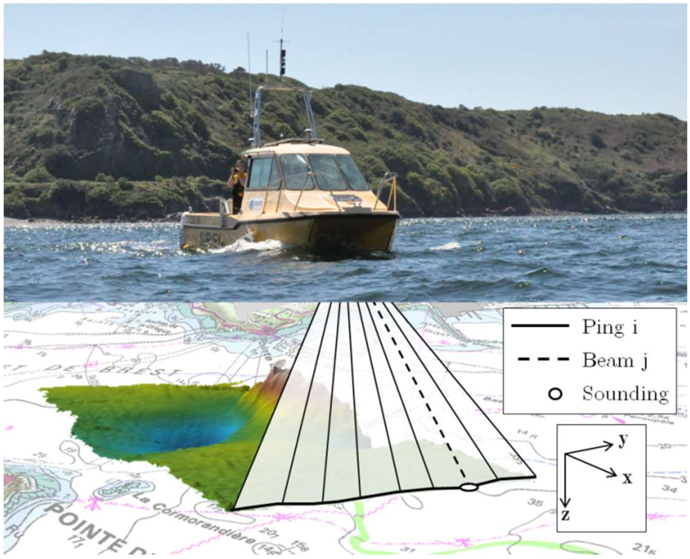
MBES are widely used in the hydrographic survey community to map the seafloor. MBES survey consists of a collection of points (i.e., soundings). Each sounding is defined by a triplet (x, y, z), where x and y represent the geographical or projected coordinates on the horizontal plane, and z the measured depth, respectively. MBES are acoustic sensors mounted on surface or underwater vehicles (e.g., Remotely Operated underwater Vehicle (ROV) and Autonomous Underwater Vehicle (AUV). Most of them are based on the Mills cross array technique for beam forming [12]. In this geometry, the transmitting array emits a wide across-track and narrow along-track beam (typically 150° to 170° by 1° to 3°). The receiver array generates a series of fan-shaped receiving beams that are in planes parallel to the ship’s direction of travel (typically 1° to 3° in the across-track direction, and 10° to 20° in the along-track direction). Echoes are detected at the intersection of transmit and receive beams either based on the amplitude or the phase shift detection of the returning signal [12]. For the simplicity of the language, each intersection of emitting and receiving beams is known as a “beam” (see Figure 2). Following a transmit/receive cycle, MBES provides a set of depth measurements (in excess of hundreds soundings depending on the model, see Table 1), by measuring sets of multiple echoes associated with their corresponding angle, in the athwartship direction. This sequence (and associated geometry is known as a “ping”. The mapping of a swath of the seafloor is then achieved as the platform progresses along its track line.
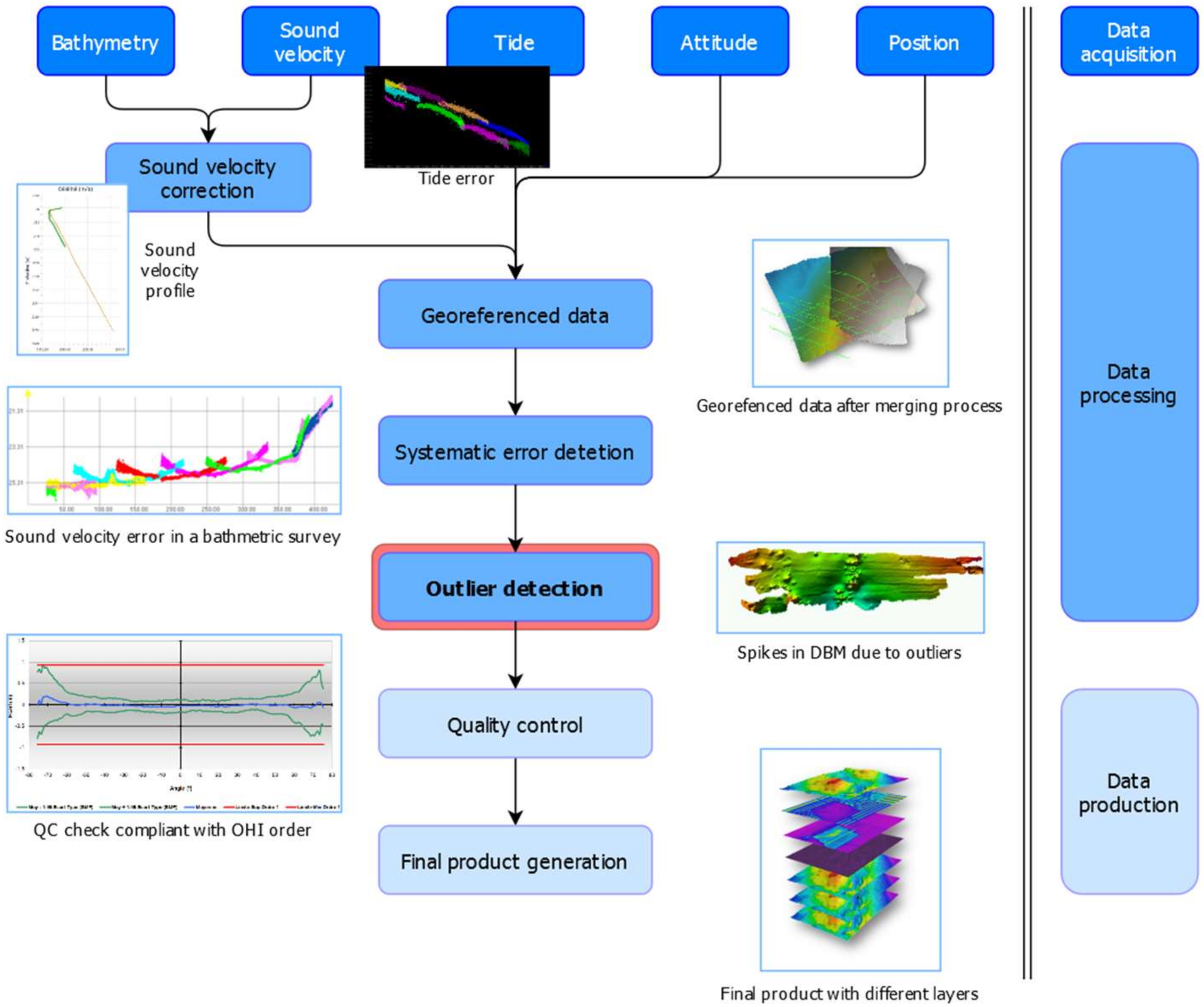
The echosounder is operated as a component of an integrated combination of sensors including Global Navigation and Satellite System (GNSS), inertial navigation system, sound velocity probes and tide gauge (or time series of the vertical height with respect to the ellipsoid). When combined together, the signal from each sensor provides the necessary information required to derive the location and depth of individual soundings. Most of these corrections are applied in real-time to ensure quality control during data acquisition. During post-processing, each of the time series per sensor is checked individually. Note the importance of a precise metrological calibration [13], which can ultimately be solved by a calibration procedure known as the “patch test” [14]. The resulting bathymetric data are then geo-referenced in the earth-based reference system to be fully exploited to be generally used in the form of Digital Bathymetric Models (DBM).
At sea, MBES data are collected along planned tracklines, which have been designed depending on the sensor characteristics (beam spacing, number of beams, accuracy of the outer beams), local depth and morphology of the seabed, along with project specifications [1]. The line spacing is set to avoid gaps between adjacent swathes and to obtain a full coverage of the seafloor. This set of MBES tracks is supplemented by one or more perpendicular tracklines, for quality control purposes.
Given the complex processes involved in the MBES bathymetric data acquisition, MBES sensor file formats store all measurements required to compute the location of each sounding from the raw data (Two Way Travel Time and beam pointing angle). Thanks to this information, it is possible: (1) to integrate into post-processing any type of measurement that was not available at the time of the survey (e.g., tide), (2) to recompute a sounding solution in case of a sensor dysfunction that was not detected during the acquisition or the availability of updated ancillary measurements (e.g., tide or sound velocity measurement), (3) to assist the hydrographer in decision-making during the validation process, as shown in Figure 3.
This set of ancillary information is often supplemented by integrating information characterizing the acoustic measurement. For example, the Quality Factor (QF) associated with each sounding depends on the sonar used, on the detection mode (Amplitude/Phase) or on the characteristics of the beamformed signal [15]. In addition, while the system acquires depth measurement, it also provides a measurement of the returning strength of the signal, known as backscatter. Texture, or seabed rugosity, and geological composition are two features which have strong influences on the backscatter signal. In some cases, it is also possible to go even further in describing the environmental context of the measurement with the storage of the water column data. However, given their huge volume, this data is not systematically recorded.
While most of the algorithms exploit only the spatial and/or temporal coherence of the bathymetric data, others take advantage of these additional attributes. Kammerer et al. in [16] suggest using the backscatter information while processing bathymetric soundings from multibeam echosounders. Calder and Mayer combine depth and horizontal uncertainties (i.e., Total Propagated Uncertainty (TPU) in their bathymetric estimator [17]. Finally, in a completely different context, Ladner et al. [18] use an a priori knowledge source Digital Bathymetric Model or “ground truth” reference to clean archival bathymetric datasets.
Swath bathymetry surveys started in the middle of the seventies. Compared to single beam systems, the first deep water echosounder, namely the SEABEAM system, allowed a remarkable increase in coverage by providing 16 depth values transverse to the navigation tracks per ping. The second generation of systems (e.g., SIMRAD/EM12 with its 192 beams per ping), which appeared at the end of the 80 s, marked a new turning point by considerably reducing the time required for surveying. With a much higher ping rate, shallow water MBES, which appeared in the mid-90 s, achieved higher density of soundings on the continental shelf and coastal areas. By collecting 127 up Table 1400. soundings per ping—for the SIMRAD/EM3000 and ATLAS/Fansweep 20, respectively—this new generation of systems makes it possible to acquire up to 400 times more soundings than the SEABEAM. In addition, bathymetric surveys conducted in 5 m of water depth with a SIMRAD/EM3000 provide on the order of 17 million soundings per hour, which represent a huge challenge in terms of data management, both with respect to real-time constraints, to data storage resources and also regarding their use as pointed out by Mayer et al. [19]. Associated with Figure 1, Table 1 presents the evolution of soundings acquisition, considering typical surveys chosen for their representative range of water depths, their type of sounders and the epoch at which the survey was undertaken, as well as their water depths and MBES systems.
In the near future, one has to consider the increasing use of unmanned autonomous vessels equipped with modern multibeam sounders [10,20]. While those are currently being positively evaluated by hydrographic offices as force multipliers, a dramatic increase in the volume of bathymetric information is to be expected, and even more so when these drones will be operated as part of a fleet.

3. Outlier Characteristics

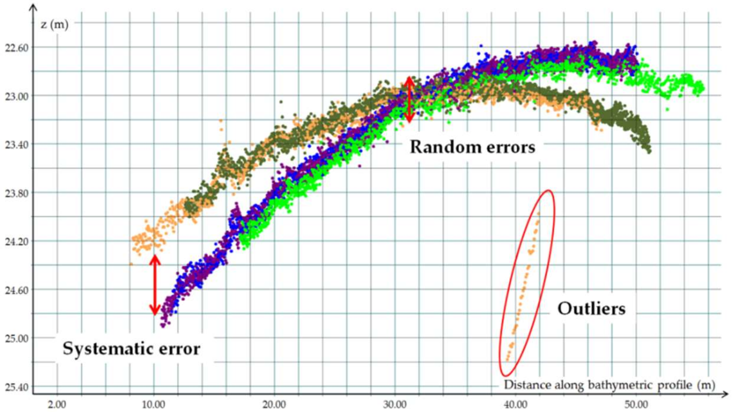
MBES soundings come with systematic errors, outliers and random errors. Calibration procedure (i.e., patch test) prior to each survey and good practices in surveying should minimize the effect of systematic errors [1]. Automatic and manual data validation should remove the impact of outliers in navigational product or DBM. Finally, random errors are intrinsic to the measurement process. Allowable limits of the accuracy of the measurement are estimated and generally evaluated according to IHO special publication n°44 [1] (see Figure 4). As stated above, our paper mainly focuses on outlier detection techniques applied to bathymetric datasets. While we are not neglecting the effect of systematic errors and random noise, we hypothesize that relevant procedures have been undertaken to minimize their effects.

3.1. Types of Outliers

The wide literature dedicated to outlier detection techniques offers a large panel of broad definitions of the word “outlier”. Most of them, though, do not give a precise definition of that term, but provide only some cataloguing of the type of outliers. Nevertheless, two formal definitions are emerging. From Davies and Gather’s point of view [21], each point of a dataset comes from a single statistical distribution. Therefore, points belonging to the tail of this distribution have to be considered as outliers. A more conventional approach postulates that two distribution laws coexist: regular samples generated by one of the distributions are contaminated by those issued from a second one from which outliers are originating. The introduction of these statistical definitions points out the difficulties of describing this term in a generic context.
Most of the time, an adapted definition comes together with the method used to detect outliers. This leads to as many definitions as there are views of the problem. Nevertheless, numerous publications also show that some types of outliers are more common than others. It is clear that the performances of the detection algorithms depend on the type of outliers encountered. Some strategies are more appropriate than others to detect a particular type of outlier and completely fail to discover another type. Therefore, the design of a detection algorithm implies knowing the main types of outliers.
Generally speaking, outliers are divided into two groups: namely gross errors or far outliers and model failure. This distinction can also be applied in the hydrographic context. Even though far outliers sometimes occur in bathymetric datasets, they are more than often filtered out as part of the acquisition process. Their presence even in small numbers, when combined with the model failure type of error can cause great difficulties to outlier techniques. Nevertheless, when detected, far outliers can be safely discarded from the dataset, since they show no coherency with the seafloor and do not require a faithful modeling of it. Additionally, named points or global outliers are mainly defined using a priori knowledge usually expressed in terms of boundaries (e.g., a priori depth or geographic extension restriction). On the opposite side, contextual or local outliers require a more accurate description of the seafloor. For that reason, this type of outlier can be put together with model failures as mentioned by Hampel et al. [22] or with spatial or relationship-oriented outliers as designated by Planchon [23]. Hydrographic cleaning is mainly concerned with this type of outliers (see paragraph below).
The distinction made between these two types artificially dissociates outliers within a dataset. In fact, interactions exist that lead to undesirable effects such as masking and swamping effects when detecting outliers. Intuitively, masking effects appear when an outlier is not detected due to the presence of another one. Swamping effects appear when a valid sounding is labeled as outlier due to the effect of nearby outliers. These two effects highlight potential problems with outlier rejection.

3.2. Outliers and Robust Statistics

In the field of Robust Statistics, outlier rejection has been a quasi-independent subfield delivering its own methodology of outlier tests. Rejecting an outlier, through these classical tests, is a decision usually made to solve a conflict between safety and efficiency. A clear outlier, possibly detrimental to the model estimation process, should be discarded if computational security is overriding. Conversely, a possible efficiency loss may occur if the rejected sample was actually a proper measurement. Setting the boundaries between rejection and non-rejection, while performing an optimal tradeoff between safety and efficiency, is thus a critical task. As mentioned in [22] Section 1.4, the identification and removing of gross errors is not always possible.
With the advent of influence functions and corresponding robust estimators, modern Robust Statistics approaches provide alternative, and more transversal, strategies to address outlier rejection. With this respect, Hampel et al. in [22] recommend performing robust model estimations through an M-estimator provided with a redescending influence function. Such estimator outputs provide a confidence attribute through a positive scalar channel attached to the measurements that continuously decreases whether an observation is a proper sample (i.e., an inlier), a doubtful outlier or a clear outlier. Actual rejections can then be a posteriori performed while setting the corresponding boundary along this curve with respect to. application-specific tradeoffs.
The statistical performances of outlier rejection techniques are evaluated for any rejection technique using the notions of robustness and efficiency initially introduced in robust estimation. In this context, robustness is assessed using the breakdown point, which is a global measure of the reliability of a method. Efficiency is measured by the influence function, which reflects the behavior of the technique near the assumed model. These two properties introduced in the robust estimation framework provide the basis for characterizing the behavior of any rejection technique. As pointed out by Hampel et al. in Section 1.4b of [22], all techniques undergo a drastic loss of efficiency as soon as the breakdown point is passed. As long as the breakdown point is not exceeded, the rejection techniques differ by their loss of efficiency. The weakness of hard rejection techniques lies in their inability to deal with both far and doubtful outliers. On the other hand, by processing data differently, robust techniques are a better trade-off between robustness and efficiency. The choice of a robust estimator (see Section 4.2) among others is based on the characteristics of the outliers in the dataset (see Section 3.3).
Finally, while performing MBES-based hydrographic surveys, the expected rate of invalid measurements barely exceeds 10%. The corresponding breakdown point can thus be safely managed through aforementioned robust estimators. In the hydrographic data cleaning framework, as discussed below, the true challenges are to propose a model:
  • Able to fully absorb proper measurements;
  • Computationally efficient;
  • Coming with a fitting algorithm suitable for the internal use of a robust estimator.

3.3. Deeper Insight into Outliers in a Hydrographic Context

Even with recent MBES technological advances, managing errors in such a complex environment remains a challenge. Several factors contribute to the deterioration of acoustic measurements or even generate outliers. It is common to gather these sources of potential outliers into two classes: (1) those specific to the platform and its movement (self-noise); (2) those induced by the environment (acoustic ambient noise). Here is a non-exhaustive list of these factors:
  • Sensors dysfunctions;
  • Bubbles at the head of the transducers;
  • Multiple acoustic reflection paths;
  • Strong acoustical interfaces in the water column;
  • Side lobes effects;
  • Bad weather conditions (low signal-to-noise ratio);
  • Objects in the water column (e.g., fishes, algae, hydrothermal plume);
  • Other equipment operating at the same frequency, etc.
Compared to a land survey, the outlier rate is higher in a bathymetric survey due to the complexity of the data acquisition process. In the bathymetric context, the outlier percentage is considered to be less than 1% for some authors [24,25], for others it is less than 10% [26], but can reach up to 25% for some tests [27]. The high variability of outlier percentage observed in the literature can be explained by the wide panel of sensors used as well as the high variability of the environmental conditions. It can also be explained by the processing context which may favor the conservation of erroneous soundings. For example, in the context of nautical charting, in case of soundings departing from the likely representation of the seafloor, the shallowest soundings are kept in the dataset, even if they can be abnormal, to ensure the safety of the navigation. Finally, if for a given dataset the outlier percentage remains unknown, because there is no ground truth, it is considered by many authors to be low [25,28,29]. It is even weaker today with MBES performances and more particularly with improvements related to bottom detection algorithms, which invalidate soundings in real time.
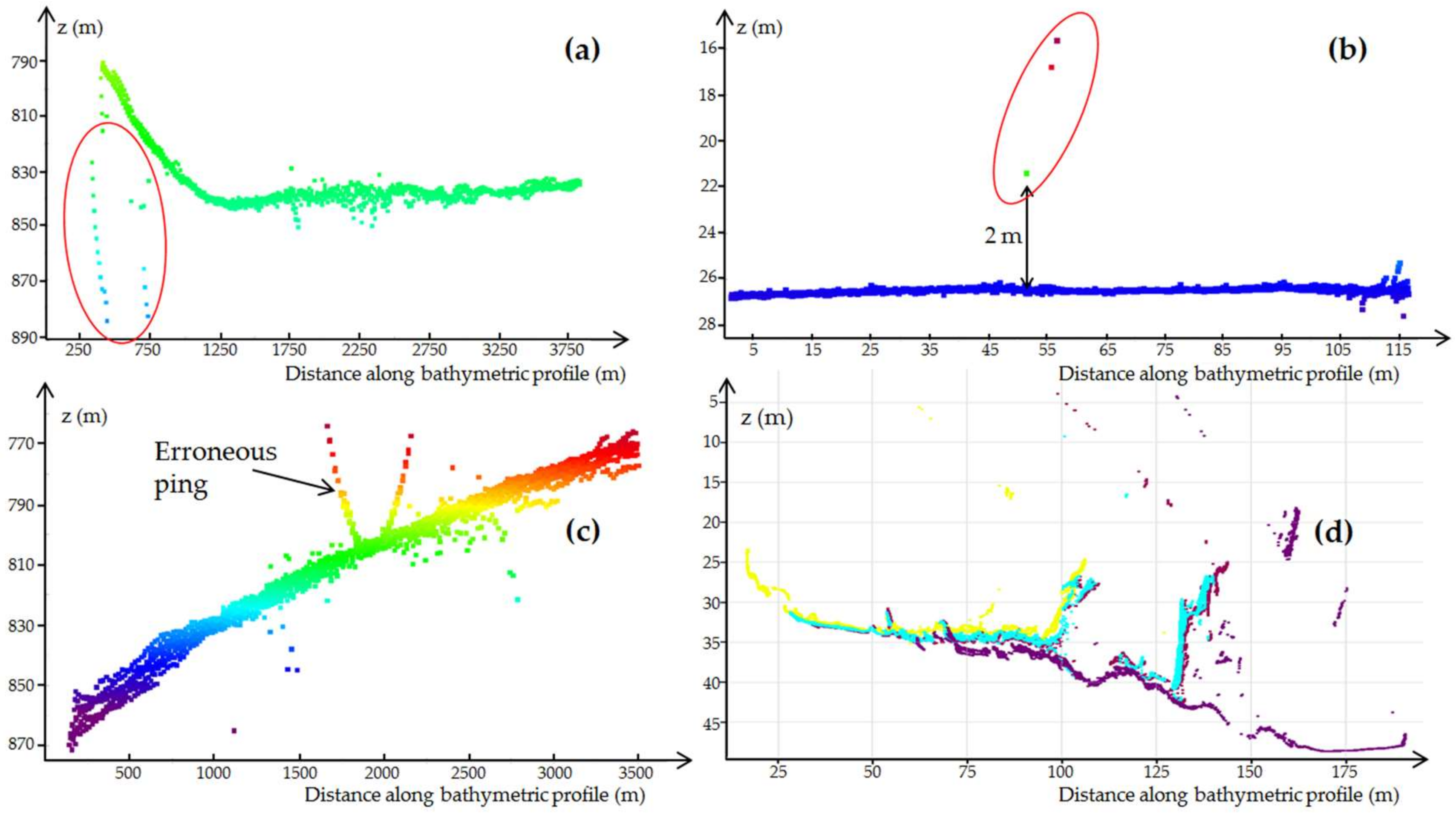
Outliers are therefore identified as being separate from the seafloor. The working hypothesis that often comes up in the literature concerns the topography of the seabed, which is supposed to vary smoothly and continuously with respect to the horizontal and vertical resolutions of multibeam echosounders [25,30,31,32]. This hypothesis is in general sufficient to allow the expert data processor to manage the various types of data in terms of quality (e.g., noise level, outlier rate) or seafloor morphology. Soundings that deviate too much from this hypothesis are then identified as outliers. However, in the field of hydrography, such a definition can be ambiguous with the characterization of obstructions or targets, which, unlike outliers, will have to be maintained in the dataset in order to be identified as local risks for the safety of the navigation. As stated by Hou [31], targets differ from outliers when neighboring soundings from different pings hit the target several times. Unlike structured objects such as pipelines lying on a flat seabed [33], distinguishing a real feature from a group of outliers is not so obvious. Figure 5 depicts four bathymetric profiles ordered by increasing post-processing complexity in the context of navigation safety. This figure displays the three most frequently identified outliers’ classes:
  • Isolated outliers (Figure 5b);
  • Structured groups of outliers (Figure 5a,c,d);
  • Unstructured groups of outliers (Figure 5d);
Some authors mention and propose to detect only one type of error, namely isolated outliers for Shaw [34], spikes for Eeg [35], Ferreira [36] and Bjorke [37] and impulsive noise for Mann [38]. Calder, Du, Li, Lu and Motao [17,27,39,40,41] oppose this first type of outliers to a second type consisting of groups or clusters of outliers or burst data, emphasizing the difficulty of dealing with them. Isolated pings or defect beams fall into this category. Hou [31] invalidate soundings belonging to an erroneous ping using a dedicated filter. Bottelier [33] and Arge [42] point out another type of structural noise which appears along navigation tracks. These ribbons of points are only one sounding thick in the simplest case, but can be more complex to process when they are dense as they become locally indistinguishable from elevated pipelines [42]. Consecutive outliers may produce geometries that can be easily identified especially for an expert who is able to choose the most suitable representation of the data (i.e., swath or geographic mode) to recognize them (Figure 5c). In a more general way, unstructured groups of outliers may require further manual investigations mainly based on the analysis of the water column data. The downhill problem described by Calder [43] falls into this type of outliers. Significant slope occurring across the swath of the sonar generates inconsistent beams which are spatially coherent and shoaler than the seafloor. Such configurations of outliers are particularly problematic for experts and automatic procedures leading to asymmetric processing in a hydrographic context, by processing soundings detected as erroneous differently depending on whether they are located above or below the surrounding seabed [25,39,41].

4. Taxonomy of Outlier Detection Techniques

The first level of classification conventionally found in methods of outliers’ detection, such as the paper of Chandola [11], is the type of supervision. The scientific literature gathers them into the three following classes, following the classic typology of machine learning algorithms:
  • Supervised: algorithms that generate a predictive function for a set of data from previously labeled data (in relation to the problem to solve);
  • Non-supervised: algorithms dealing with unlabeled data, in other words, with no prior knowledge of the data;
  • Semi-supervised: algorithms merging these two approaches by determining a prediction function for the learning step with a small amount of labeled data and a great amount of non-labeled data.
In the hydrographic field, the majority of outlier detection algorithms are based on non-supervised methods. No semi-supervised method has been identified and only two supervised methods based on Deep Learning exist. However, only one of these two techniques has been the object of a scientific publication [44]. Therefore, the present survey will provide a deeper insight into techniques belonging to non-supervised algorithms.
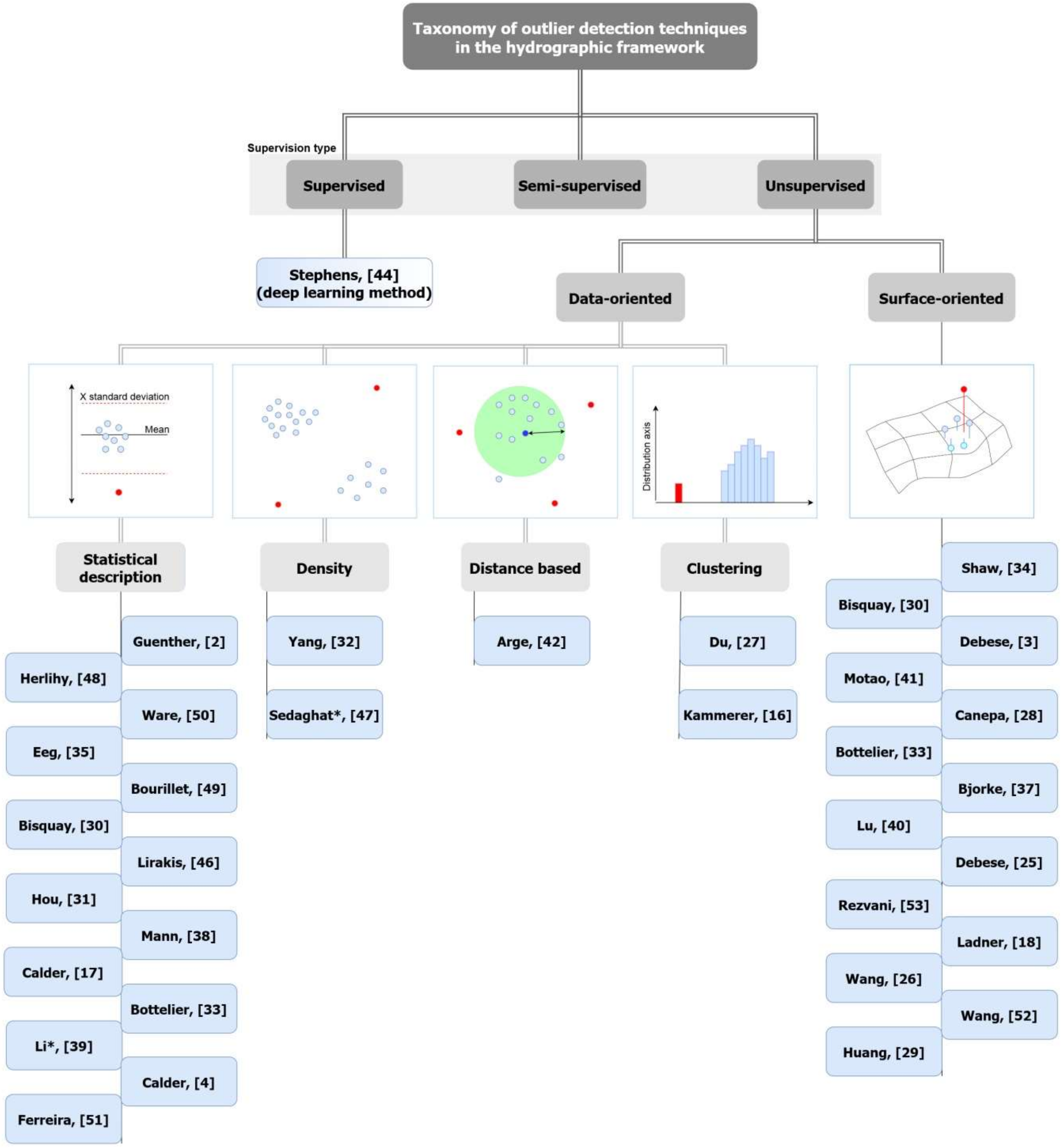
Non-supervised techniques only suppose that errors are separated from the ‘normal’ data and will appear as outliers [45]. Techniques belonging to that class can be gathered into two subclasses: (1) data-oriented or diagnosis approaches which point out outliers by working directly on data, and (2) surface-oriented or accommodation approaches which robustly build a model of the seafloor from all the points before detecting outliers.
The first level of the comprehensive taxonomy framework under investigation is based on these classes. As shown in the next two paragraphs, such an approach provides a detailed description of the different algorithms while highlighting their similarities and differences.

4.1. Data-Oriented Approaches

According to data science [6], data-oriented detection techniques are broadly classified into the four following classes:
  • Statistical-based approaches are generally divided into two classes depending on whether the distribution of the data is assumed to be known or not. Parametric approaches are used to estimate the parameters of the assumed distribution, most of the time the mean and standard deviation of a Gaussian distribution, while non-parametric approaches estimate the density probability from the data, without any assumption about the shape of the distribution. In both cases, outliers are identified as points belonging to the ends of the distribution tails.
  • Distance-based approaches, also called nearest neighbor techniques, rely on the spatial correlation by computing the distance from a given point to its vicinity. Points having a higher distance than other normal points are identified as outliers.
  • Density-based approaches are quite close to distance-based approaches, as the density of points per unit of surface/volume is inversely linked to the distances between neighbors. Outliers are localized in low-density areas while normal points are aggregated.
  • Clustering-based approaches are classical approaches in machine learning. These global approaches consist of grouping similar data into groups called clusters. Since outliers are rare they are either left isolated or if they are grouped into a cluster the latter is far away from the others.

4.1.1. Statistical-Based Approaches

As highlighted in Figure 6, statistical approaches are by far the most numerous, and also the earliest. The first approach, better known as the Combined Offline Processing (COP) program was proposed by Guenther in 1982 to improve the selection of soundings acquired by the BS3 swath system [2]. As shown in Table 2, data-oriented approaches have been grouped by class (see Section 4.1) and then according to their overall structure. The latter is based on the number of techniques developed by the approach, either one or several. When the number of techniques proposed is greater than one, the grouping is made according to whether the techniques are cascaded or implemented independently of each other.
Four approaches are based on simple cascading filter [46,47,48,49]. The number of filters varies from 3 to 5 depending on the approach. Most of these filters operate in swath mode with no need to define the size of the neighborhoods, which are directly fixed by the approach. The only parameter to be set by the operator is, if necessary, the size of the group of pings to be processed [46,47,48]. The common basic filters make use of the depth or cross track distance gates [46,47,49] or the number of non-zero neighboring soundings [46] to detect erroneous soundings. The statistical filters implemented in these approaches are primarily based on the calculation of mean or standard deviation values. Bourillet in [49] proposes to invalidate a ping by thresholding the difference of mean values between pings computed in 3 × 3 boxes. Ware in [50] pre-flags the data by sorting them into eight classes built from weighted mean and standard deviation of depths. Each of the three filters proposed by Hou in [31] relies on dispersion measurements. Its first filter combines the global variance representing the seafloor trend of a group of pings with the local variance measured around each sounding to detect erroneous soundings. The second test compares the local variances of two local neighborhoods built up with and without the sounding to be tested. The third one is designed to detect erroneous pings. The covariance filter proposed by Lirakis in [46] also falls into this category. This filter is the first of a series of five filters that progressively change the status of all data. Soundings detected by the covariance filter are marked as ‘bad’ data, while those identified by the sifting filter as belonging to the main mode of the 2D histogram representing the distribution of the roughness and slope are marked as ‘good’. The remaining unknowns are then classified as ‘bad’ or good according to a two-stage local validation process. Unlike all other multi-pass filtering approaches, the data are at this point converted into geographic mode for further statistical filtering.
Six out of fourteen existing statistical approaches are based on a single algorithm. The statistical filter proposed by Guenther which is based on the mean and a multiple of the standard deviation of depth values falls into this category [2]. This algorithm is the only one in this category to process the MBES data in the swath mode by fixing the window size according to the studied MBES bathymetric dataset. All the others are operating in the spatial mode [4,17,35,38,50]. The size of the neighborhood is then a user-defined parameter except for Egg. The resolution of the regular grid which defines the neighborhoods used to perform the statistical tests in [4,17,50] is replaced by the first-order neighborhood of the TIN (triangulated irregular network) built from the data projected onto the horizontal plane. While this approach has the disadvantage of eliminating swath edge soundings or soundings distant from the surrounding data from testing, it offers the advantage of statistically checking the neighborhood validity. The in-between approach proposed by Mann [38] defines the neighborhood by setting the number of the closest neighboring soundings of a point. The approaches of Egg, Guenther and Mann work in a similar way by testing the soundings one by one. Once selected, a sounding is compared to a statistic estimated from the data of its surrounding neighborhood. Egg detects spikes by applying leave one-out testing scheme that estimates the contribution of a sounding to the local seafloor variation. Finally, Mann applies a median filter to detect outliers. The last algorithm of this category is the one proposed by Calder and commonly known as the Combined Uncertainty and Bathymetry Estimator (CUBE) algorithm.
CUBE is an error model based on the computation of DBM which estimates potential depth values associated with a confidence interval for each node of the DBM. The algorithm works in three steps. The first step prepares the data for each grid node, by associating to each sounding measurement an estimate of its TPU. The second one is generating hypothesis of higher likelihood of where the seabed should be for each grid node. The third one is a disambiguation phase where multiple hypotheses may exist. As part of this stage, the algorithm presents to the hydrographer alternative seabed hypotheses if the sounding dispersion is too important. This algorithm is widely used by hydrographic national organizations, such as the National Oceanographic and Atmospheric Administration (NOAA) and at the Canadian Hydrographic Service (CHS). However, limitations with this algorithm are well-known, such as poor behavior in the case of chaotic seafloor (rocky areas or obstructions). In this case, the number of hypotheses significantly increases requiring the intervention of the hydrographer. It is strongly recommended to undertake a quick manual pre-filtering on the data prior to use this algorithm. In order to take into account those limitations, an improved version of CUBE is proposed with CUBE with Hierarchical Resolution Techniques (CHRT presented in [4]) including multi-resolution of DBM (adapted to areas with higher variability), multi-processing (to improve performances) and taking into account the Quality Factor [15] (see above, in order to better estimate the TPU).
The last three statistical-based approaches implement several algorithms [30,35,36]. Another common point that links all these techniques to each other is their implementation of geostatistc techniques. The latter have a high computational cost. Providing the user with various companion techniques is thus relevant. Such techniques can address (1) the measurement of their performance against simpler techniques [30], (2) the simplification of their implementation [33], (3) a better exploitation of their results [36]. Bisquay [30] implements (together with the kriging technique detailed in Section 4.2) two simple methods. All the proposed techniques operate in geographical space. The depth increments method looks for obvious outliers inside a swath. By working on swath covering areas, the quantiles method detects much more outliers. These two techniques are much less time computing than the cross validation technique and are a prerequisite for its implementation. The 1D and 2D cross validation methods proposed by Bottelier [33] are respectively applied on a ping and a dataset of at least three pings and three beams. Compared to the robust kriging interpolation technique described in Section 4.2, these two techniques are faster with significantly reduced performances. The third and last approach based on geostatistics is the one of Ferreira [36]. Previous to its application, an exploratory analysis is carried out to check for the spatial independence of the depth data. Unlike the technique proposed by Bottelier, which predicts the depth of a sounding from its vicinity by modeling the spatial structure of the data using a semi-variogram, Ferreira applies segmentation in circles. A spatial analysis is conducted for each sounding from the residual depth values of the soundings of its centered circle neighborhood. The modified Z-score method, δ method and boxplot method are independently applied to identify outliers inside each subsample circle. By construction, a sounding can be detected as an outlier more than once. Each of the three techniques assigns to each sounding a probability of being an outlier. The performances of these techniques are data dependent [36,51].

4.1.2. Distance-Based Approach

A topological-oriented approach involving non-local neighborhoods between vertices of a special graph is proposed in [42]. First, the measurement points are described as the vertex set of a planar graph provided by the 1-Skeleton of their Delaunay triangulation. Then, for any adjacent triangles pair, an edge linking the two opposite vertices is also added to the initial graph. Finally, every edge involving a depth change greater than a given threshold is removed from the graph. Each connected component of this graph can then be identified as a potential cluster of outliers. This partition allows discriminating spikes from coherent structures above the seabed (e.g., pipes, wreck).

4.1.3. Density-Based Approach

Two approaches make use of a density-based scheme [32,47]. The first method consists of projecting the data along the orthogonal direction and side direction respectively in the MBES frame. All the data, now on the same plane, are mapped into bins. The largest region of seabed data is identified by searching for the densest bin, then increasing the size of the region with adjacent bins. Then a classical image processing erosion and dilation algorithm is used to locate the outliers that are connected to the seabed data region. Anything outside this seabed data region is then considered as an outlier. Finally, each ping is also filtered using a statistical method on a local study window. This density method also uses innovative image processing techniques that are not often seen in the methods studied. Segaghat in [47] uses a combination of two algorithms well-known to the scientific community of data processing. His technique is based on a density computation, using as an outlier detection algorithm the Local Outlier Factor (LOF) and density-based spatial clustering of applications with noise (DBSCAN). These two algorithms are combined to find spatio-temporal outliers, where the temporal adjective means that it remains present throughout time (typically months). LOF algorithm was designed as a relevant alternative to [32] algorithms as it detects outliers depending on the local neighborhood of the point observed and gives an anomaly score for each sounding. The parameterization is carried out by setting a threshold on the maximum authorized anomaly value. In his paper, Sedaghat has optimized this parameterization in order to minimize false detection with respect to the dataset under study.

4.1.4. Clustering-Based Approach

The two approaches proposed by Du in [27] and Kammerer in [16] belong to this category.
Du’s technique works in the swath representation mode by cascading three filters. The first filter applies a depth gate to a working window consisting of a group of consecutive pings. A coarse-to-fine approach that mimics an operator’s decision-making is then applied. It starts from building a depth histogram over the working window. The soundings dataset is then partitioned according to the modes of the depth histogram. The secondary modes having a sufficient gap with respect to the main mode are identified as outliers. The working window is shrunk by decreasing the number of beams and the process is repeated. This recursive approach ends by applying a Dixon-test to a group of six sounding while cleaning a ping.
The approach proposed by Kammerer [16] differs from all other approaches proposed in this survey as it operates on MBES backscatter data. Four independent algorithms are implemented to detect high and low backscatter zones. The histogram, entropy and the Fuzzy k mean segmentation work in a ping-to-ping representation mode, while the later uses a neural network based texture analysis of a mosaic. These algorithms provide imagery-derived zone boundaries that are visualized together with the positions of the soundings declared dubious by a MBES data-cleaning algorithm. Such tools are helpful in a hydrographic context when one has to preserve the obstructions for navigation safety.

4.2. Surface-Oriented Approaches

These approaches are based on a seabed modeling. Soundings departing from this surface are considered as outliers. As shown in Table 3, this methodology relies on the choice of:
  • A mathematical model that describes the set of features that are the most representative of the seabed morphology;
  • A robust approach that takes into account the presence of outliers and assumes an a priori random noise while estimating the model parameters;
  • A strategy that identifies outliers as a subset of distant soundings far from the model.
The methodology to compute the model is essential in this approach. It should reflect the morphological variability while still isolating soundings to be considered as outliers. The approaches proposed in the literature fall into two categories. Global approaches fit a trend surface on the overall area covered by the survey, whereas local approaches operate through a preliminary partition of this area and then independently fit a local trend surface on each element of the partition. Consequently, the global approaches stress on the ability of a flexible trend model able to account for the complexity of the seabed morphology. By reducing the geographical scope of their model, local approaches can rely on simpler models provided that the partitioning has been performed adequately with respect to the seabed topographic changes.
To create a global surface despite the presence of outliers, different approaches can be considered.
One of them implements a coarse-to-fine strategy. Shaw [34] uses a global optimization procedure to find a stable surface shape. The bathymetric surface is obtained by minimizing an energy function that combines three competing constraints for surface smoothness, continuity and adherence to the soundings. The Graduated Non-convexity algorithm is applied to achieve the minimum-energy surface. Rather than minimizing the energy function directly, which is impracticable when the number of outliers is high, this algorithm minimizes a convex approximation of the energy function. This coarse approximating energy function is iteratively refined until it approaches the true energy function. Once the minimum-energy surface is obtained, outliers are identified as deviation points.
Another coarse-to-fine strategy is proposed by Bjørke [37]. Unlike the previous one, which processes the bathymetric data in swath mode, Bjørke applies an average interpolating subdivision technique to extract the seafloor trend surface in the geographic mode. A fine regular grid of cells is firstly defined and partitioned into square blocks. Soundings are assigned to a cell in the fine grid and an estimation of the average depth over each block is computed. A polynomial function is then constructed over a block and its eight surrounding neighbors, where the mean value of the polynomial over each block is equal to the block average. The average values of the four sub-blocks of the center block are predicted by integrating the polynomial. This procedure is repeated until the sub-blocks have the same size as the cells of the fines grid. The resulting trend surface is then used to filter out outliers.
The approach proposed by Canepa [28] also follows a coarse-to-fine strategy but unlike the two previous approaches the detection of outliers is carried out simultaneously with the construction of the global surface. A triangulated map is built with respect to both the seafloor topography and data noise amplitude. The mesh is initialized with the plane triangular facets passing through the vertices belonging to its convex polygonal contour. This linear piecewise continuous approximating surface is iteratively refined by adding at each step the data point with the maximum error. The outliers are identified before updating the mesh. Two algorithms are applied. The first one, which is based on the fourth-spread range test, flags the far outliers. The second one performs a robust local polynomial fitting using Tukey’s biweight M-estimator and provides the smooth value of the point that will be added to the mesh.
Alongside this coarse-to-fine strategy, other techniques have been considered to produce a flexible and global trend surface.
Bottelier [33] makes use of a robust interpolation technique to produce a global smooth surface of the seafloor. The Kriging technique remains used as the interpolation method. As a hypothesis, the measurement accuracy is the same whatever the observation. The spatial dependence of the data is modeled with a Gaussian covariance function by setting its correlation length to the average points distance between the points. The robustness is achieved by iteratively removing the influence of outliers from the over-determined kriging system of equations. To this end, a nugget effect is assigned to each observation. Its update is computed as a weighting function of the observation residual value.
Huang in [29] implements a sparse weighted Least-Squares Support Vector Machine technique to construct a seabed trend surface that reflects the overall change of the seabed topography. The robust trend surface is obtained by minimizing a cost function that contains two terms. The first term measures the goodness of fit of the model while the second term, also called the confidence term, enforces the smoothness of the model. The surface model is built as a weighted sum of Gaussian Kernel functions to account for significant bathymetric variability. The optimal value of the Gaussian kernel parameter and the regularization parameter, representing respectively the tradeoff between closeness and smoothness, are obtained from a training dataset by solving a linear system. The coefficients of the support vectors, which represent the influence of each training data, are then robustly re-estimated from a weighting function of their residual values. The support vectors with the smallest influence are then removed and the previous steps are repeated until a user defined performance index degrades. However, native SVM approaches are known to have a high computational cost. Wang ([26,52]) proposes heuristics algorithms aiming at working through a reduced set of support vector machines, still using radial basis kernels and robust metrics.
Unlike global approaches, the models on which local approaches are based can be much simpler since their spatial extent is limited. All approaches belonging to this category rely on polynomial surfaces of degrees 0 to 3. They differ in the techniques used to define the size and shape of the working neighborhood. There are two groups of approaches. The point-based approaches define a neighborhood for each sounding to test, while the area-based approaches first subdivide the survey area into blocks before fitting a local trend surface over each block and pointing out outliers.
The approaches proposed by Shaw and Motao fall into the first category. The Robust Linear Prediction algorithm implemented by Shaw [34] is an adaptation of an image restoration technique. In its first form, the algorithm successively examines the soundings of a swath. The sounding depth is computed using an M-estimator defined as the weighting sum of the soundings belonging to its non-symmetric half plane (x,y) support neighborhood. If the sounding is invalidated, its depth is replaced by the robust predicted value. The process is repeated until the end of the swath. Finally, Bisquay in [30] applies a kriging-based interpolation technique to locally model the seafloor topography using a random function of order 1. Robustness is introduced by the application of one of the two filters proposed by the method in order to eliminate far outliers.
The approach proposed by Motao in [41] is similar to the previous one with the difference that the soundings are represented in the spatial mode. The sounding depth is computed as an inverse distance weighting average of the neighboring depths. The robustness is introduced by replacing the neighbor’s weights with their equivalent using the weighting function of the IGGIII M-estimator. The key point of this iterative reweighting least-squares approach is its initialization value which is set to the median of the sounding depths over the predefined neighborhood.
Like the two previous point-based approaches, the area-based approach proposed by Debese [3] makes use of an M-estimator. The geographic area is first divided into squared cells of identical size. Tukey’s biweight estimator is applied to each patch to estimate the parameters of a quadratic surface and detect outliers.
Rezvani [53] applies a similar approach to reduce the huge volume of bathymetric datasets while constructing a DBM. The depth is estimated on each cell using a horizontal plane as the weighted average of the soundings it contains. The approach was applied by testing four different M-estimators, including Tukey’s biweight and Huber estimators which achieve the most efficient results.
These two approaches are based on a regular division of the area and assume that the chosen local model is statistically valid. For cells whose size is not adapted to the chosen model, the detected soundings reflect the inadequacy of the surface to the data. Debese [25] proposes to automatically adapt the cell size by performing a descending quadtree subdivision using rules based on both statistical and spatio-temporal inferences. This multi-resolution approach provides a set of outliers together with a classification map that highlights areas of concern.
As a result that they provide a good trade-off between performance level and computational cost, M-estimators are by far the common choice when carrying out robust regressions. However, other estimators are theoretically more robust, as for example, the Least Trimmed Squares (LTS) estimator used by Lu [40] to fit bathymetric data using geospatial arrangement. The breakdown point of the LTS estimator is determined through its trimming constant setting. It defines the fraction of the input data points (at least 50%) used to find the optimal subset that is the subset providing the minimal sum of squared residuals. Meanwhile, its large combinatorial search space may require additional heuristics to moderate its computer requirements. To this end, Lu limits the fittings to successive swath temporal windows.
Figure 6 displays the repartition of existing approaches, presented in this Section. All of the cleaning algorithms described below are listed in this classification.

5. Output of Outlier Detection

Finally, following the Chandola [11] classification, this section will focus on the outputs of the detection algorithms. Moreover, in the hydrographic context this aspect is essential. It is in fact necessary to ensure that the shoal soundings are preserved and noticed on nautical charts.
Outlier detection techniques are carried out with different objectives. The first one aims to provide a set of validated soundings while leaving aside the creation of DBM, preserving soundings of importance for the benefit of navigational products. The purpose of the second objective is to construct a seafloor model while detecting outliers with a regular gridded surface [17,41] or a triangular irregular network [28]. These approaches were developed to meet the expectation of different application contexts such as efficient size reduction of bathymetric datasets [28] or the preservation of manmade structure such as pipeline [33,42].
In the first objective indicated above, aiming at data validation or data sorting, the outlier detection techniques are gathered into two types according to the way outliers are reported [11]:
  • Scores techniques (regression);
  • Labeled techniques (classification).
The first type of techniques assigns a score to each outlier to denote the outlierness degree of a sounding. This outlierness measure gives rise to a ranked list of detected soundings requiring the intervention of a hydrograph to decide whether a doubtful sounding must be invalidated or not. The content of the list may be fully observed pulling out the soundings in decreasing order, or, partially observed, applying an outlierness threshold [3,26,36,41,50]. This first approach was historically preferred as hydrographic services are responsible for navigational security [2]. Today, high volumes of data tend to turn the outlier detection techniques into the second type of approach in order to maintain the ratio between acquisition and processing time close to one [5]. Detecting erroneous soundings belonging to the first type of outliers (§3.1) is not a problem as inconsistent soundings are far outliers detected by setting wide bounds around the system range or the seafloor depth. Carrying a binary decision to these abnormal soundings is a good solution.
A third type of outlier detection techniques is introduced in hydrographic data processing based on a hybrid approach [17,54]. It can be considered as a trade-off between processing time and navigational security constraints requiring manual control over litigious areas. Taking advantage of recent technological advances such as 3-D and/or multi-attributed visualization, outlier detection techniques give a more important place in the definition of objective criteria—making use of the acquisition system specificities—to make the hydrographer decision easier and more objective.

6. Summary and Discussion

Since the use of the first deep water MBES systems (e.g., SEABEAM) in the early eighties, more than seventy studies have been conducted to automatically detect and invalidate erroneous soundings in MBES bathymetric datasets. The development of automatic approaches increased in the beginning of the late 90s to early 2000s with the use of shallow water MBES systems. The huge volume of bathymetric datasets combined with the emergence of new issues in marine environment led to create much more complex approaches in place of the basic filtering techniques that were firstly developed.
Our study mainly focuses on 33 of the 70 approaches initially identified. These papers were selected based on their accessibility (i.e., language), availability (i.e., internal reports) and their originality (no redundancies in the papers selected here). We have therefore kept only one scientific paper per original data processing method even though many variations in parameterization or use may exist. In addition, the publications describing the successive advances in the work carried out by a research team were limited to those outlining the important stages of their progress. Slightly less than half of the approaches (15) were published in a scientific journal, all the others were published in the proceedings of an international conference. According to our classification, among the 33 approaches, 19 were classified as data-oriented methods while the remaining approaches are classified as surface-oriented methods. As pointed out in paragraphs Section 4.1 and Section 4.2, the statistics presented in this section refer to an approach and not to an algorithm: an approach may have led to the development of several algorithms. This section provides a perspective on the historical and conceptual improvements of these techniques, while attempting to set the scene for future developments.
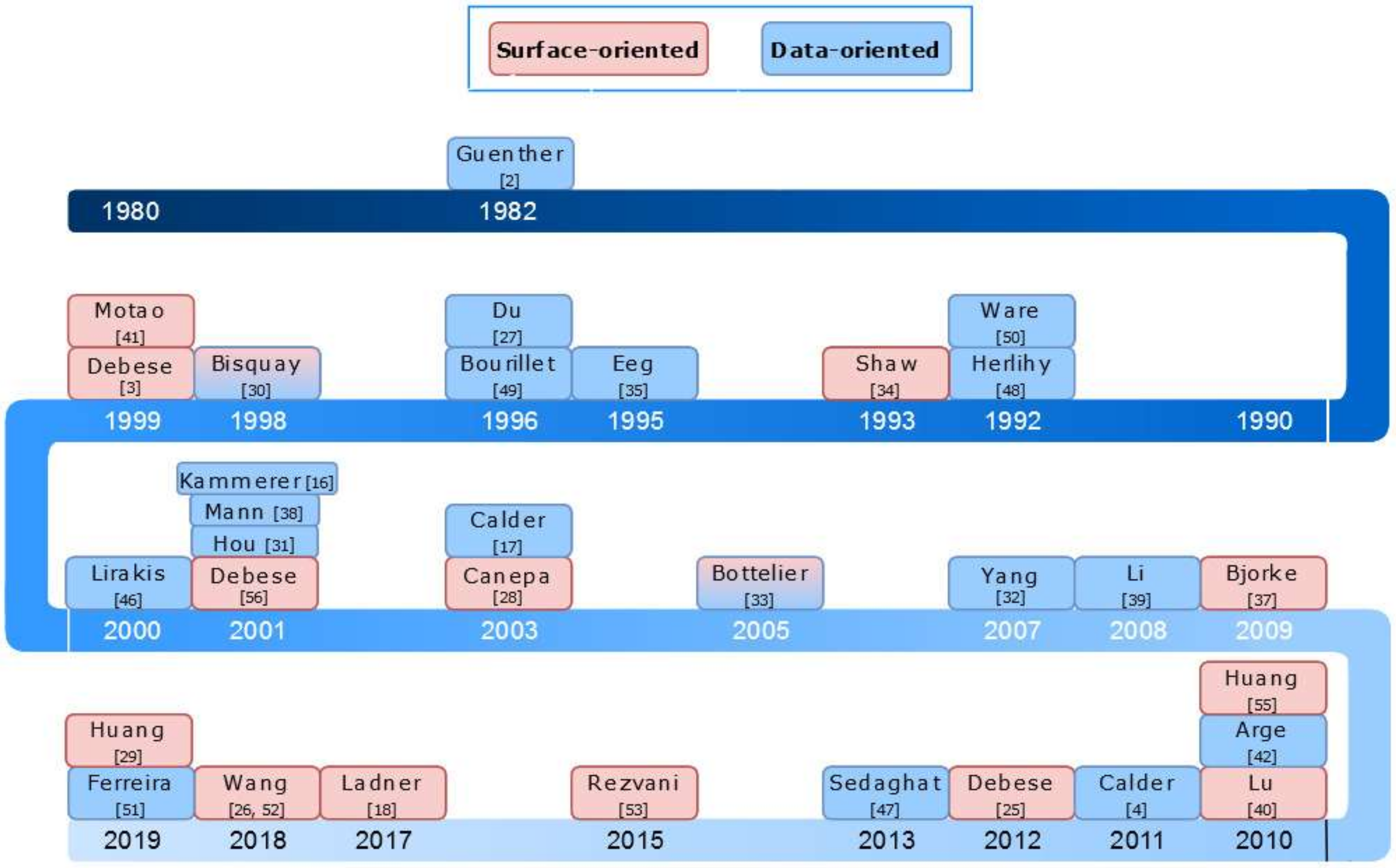
Figure 7 displays evolution over time of these techniques according to whether they belong to data-oriented or surface-oriented classes. This clearly shows that the first algorithms mostly belonged to the data-oriented class. Techniques based on surface estimation mainly appeared in the late 1990s and early 2000s. The end of the 2000s shows a new impetus in scientific publication with, in particular, the advent of CUBE algorithm [17]. The 2010’s were an opportunity to see improvements in the techniques of the 2000s (see [4,25]) as well as the emergence of techniques associated with artificial intelligence technologies (and more particularly machine learning subset) [29,44,55].
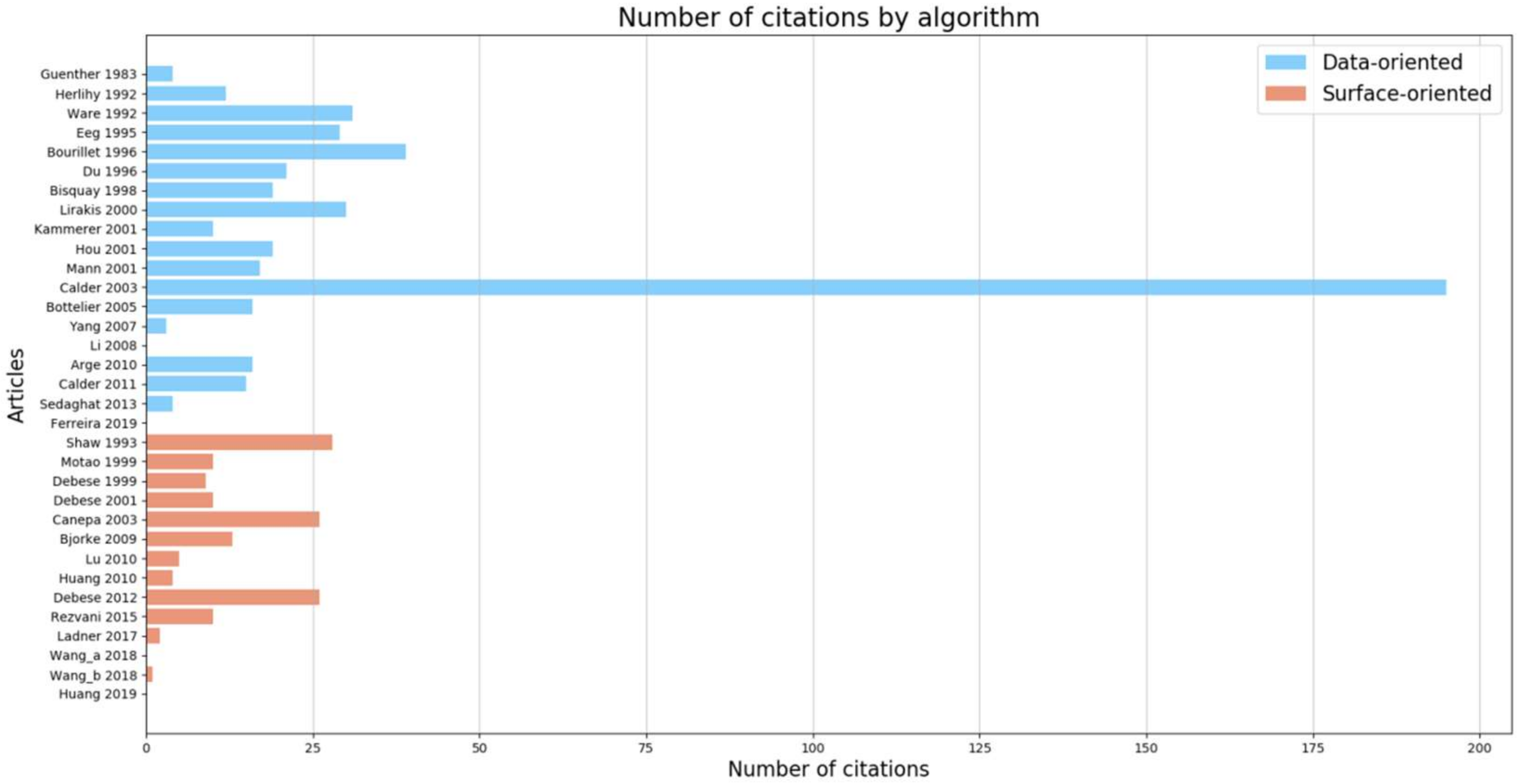
Figure 8 shows statistics related to the number of citations (as reported by Google Scholar) of the algorithms detailed in this survey. Data-oriented methodologies are represented in blue, while surface-oriented are in orange. This figure clearly illustrates that the CUBE algorithm is the most used and cited technique. This is explained by the fact that this technique has been implemented in multiple commercial software, hence favoring its use by major national hydrographic organizations. In addition, only the original article detailing the CUBE algorithm and its adaptation to a variable resolution scheme [4,17] have been retained in our survey, while a number of explanatory papers and examples of use of the algorithm on various datasets, have not been considered herein. Apart from the CUBE algorithm, a number of other highly ranked citations are essentially based on a data-oriented techniques with the exception of Debese [25,54], Canepa [28] and Shaw’s [34].
Being a key element in the development of an outlier detection technique, the representation of the bathymetric information will be discussed first. As presented in Section 2 the MBES bathymetric data can be either seen from a spatial perspective (i.e., x, y, z triplet) or from a temporal/sequential perspective (i.e., ping/beam). Each representation has a different influence on the way the neighborhood under study is considered. As shown in Figure 9a, data-oriented methods commonly use one type of representation or another, with no particular tendency (i.e., 9 sequential and 9 spatial). Notably, only [16] uses a dual representation. On the other hand, for surface-oriented methods it can be seen that the majority of the authors uses a spatial representation (i.e., 9 algorithms) of the data or a dual representation (i.e., 5 algorithms) and only two use the sequential representation [34]. This difference between the two main families of techniques can probably be explained by the fact that the surface-oriented methods are based on a seabed modeling, which by its nature is described in geographical space. Surface-fitted techniques that work in the temporal space do not take advantage of the overlap between swaths and more importantly leave out some corrections (e.g., the yaw) distorting the description of the seabed.
The type of outliers is one of the major key components of a detection technique. Section 3 describes first the two common types of outliers before focusing on outliers specific to MBES bathymetric data. Most outlier detections start by identifying and processing far or “global” outliers. Data-oriented approaches mainly use a depth gate filter [27,33,46,48,49], while most surface-oriented approaches apply median-based filters to cope with far outliers [17,25,26,28,30,41,53]. Most approaches address all types of “local” outliers with the exception of Eeg’s approach [35] which is devoted to spikes detection and those proposed by Hou and Bourillet which detect erroneous pings [31,49]. In the context of navigation safety, the distinction between outlier and object is generally handled in a posteriori and manual stage, except for two approaches [25,31].
As mentioned in the previous section, two types of output can be considered to define an outlier: the scores techniques (i.e., regression) or labeled techniques (i.e., classification). As highlighted in Figure 9d, the majority of data-oriented approaches make use of labeled techniques (i.e., 14 algorithms) while only three of them are based on regression methods. Conversely, the ratio between classification and regression technique is almost equivalent in the case of surface-oriented approaches with eight and six approaches, respectively. The hybrid approaches of Calder and Debese are an alternative to these two main types of techniques by providing output maps [17,25]. Both CUBE number and strength hypothesis maps and CHARM [25] classification map highlight litigious areas that will require further manual investigation.
The performance of an algorithm can be evaluated according to different criteria such as the quality of its results (i.e., robustness), its computational time (or tractability). The number of parameters, their ease-of-adjustment as well as the availability of a posteriori control of the parameters setting, have to be taken into account in an operational context. The number of parameters varies greatly from one approach to another. In some cases, no parameters are required as the approach is dedicated to a specific sounder [2]. Data-oriented approaches based on cascaded techniques may require the adjustment of more than eight parameters [48]. There are usually two types of parameters: those related to the definition of the neighborhood and those inherent to the technique. The parameters related to the definition of the neighborhood depend on the data representation mode. In the swath representation mode, the user has to set the size of the packet of pings to be processed [27,31,46,48]. The filters are then applied either per ping [27,33], per pair of consecutive pings [46] or on rectangular windows whose size is a priori fixed or adjusted automatically by the approach [27,31,46,49]. In the spatial representation mode, the user has often to provide the grid resolution [17,25,37,49,50,53]. Bisquay in [30] and Ferreira in [36] define the neighborhood by a search radius around the sounding to be tested. Eeg in [35] and Mann in [38] make use of the spatial structure of the data (i.e., by building a TIN) to create their working neighborhoods. In the latter case, the parameter defining the neighborhood is the number of closest neighbors. Additional criteria can be included to refine the geometrical construction of the neighborhood such as the minimum amount of data [30,35,48], or to design the variable neighborhoods for adaptive approaches [4,25,37]. Finally, some approaches such as those of Debese and Eeg propose a global a posteriori control of the neighborhood setting. As with any type of approach, a distinction is made between the model parameters that are intrinsic to the technique and those measuring the deviation from the model. The parameters specific to a technique are more or less numerous and above all more or less intuitive, requiring advanced-user knowledge or at least the definition of predefined configuration files (see the benchmark discussion below). The vast majority of data-oriented and all surface-oriented algorithms require the user to set the detection threshold as a scale factor of the standard deviation.
Another relevant element to investigate is the type of dataset used to test the processing methods (see Figure 9b). The major part of data-oriented approaches (i.e., 15 amongst the 19) were evaluated on real datasets while the remaining four were tested both on artificial and real datasets. The proportion of surface-oriented approaches performed only on real data is slightly weaker (i.e., 10 amongst the 14).
Table 4 presents the main characteristics of real datasets associated with the testing of the methods we studied in this paper. Amongst these characteristics we have retained the range of depth, the sounder technology, the volume of the dataset in terms of number of soundings, as well as the type of the dataset (i.e., A: for area, S: swath line; P: group of pings).
The performances of all the algorithms with the exception of those described in [39,47] were measured on MBES datasets. Li and Sedaghat data-oriented approaches were tested on SBES datasets. Being much easier to install and also less expensive, SBES are commonly mounted aboard a number of opportunity vessels (i.e., transit lines, from ferries or shipping vessels, etc.) to produce crowd-sourced bathymetry datasets. Driven by the growing phenomenon of Volunteered Geographic Information (VGI), Sedaghat implements an approach in the context of navigation safety in a port environment [47].
Volumes of bathymetric datasets used to test the algorithms show a wide disparity ranging from a few numbers of successive pings (i.e., 1045 soundings) to more than 23 million soundings. With the increase of sampling rate of recent sensors, it seems important to consider algorithm, which have been tested on a sufficient amount of data, in order to assess their practicability in terms of computational efficiency.
Real bathymetric datasets, taken as a whole, cover the full range of water depths. A high number of approaches has only been tested for shallow water data (i.e., 18). Five approaches have been evaluated on both deep or very deep water depths. Only one approach has been assessed over the full range of water depth [3,56].
Artificial datasets are useful for didactic purposes to describe the steps of an approach [25,28,31,37,38,55] or to explain the influence of the parameters on detection results [25,28,40,41,53]. The size of these artificial datasets varies from a few tens or hundreds of points [29,31,37,41] to tens or hundreds of thousands of points [25,28,53]. Artificial datasets built for illustration purposes are limited to a sample that is quite far from reality [29,37,38,41] or even only defined in 1D [28,37,55]. When the objective is to conduct a deeper analysis of the algorithm behavior a panel of three to four synthetic bathymetric datasets that mimic the variety of seafloor morphology is built. The strategy currently used to create these datasets rely first on the choice of a relief model from a horizontal plane [41], polynomial model [25,53] or more complex analytical functions [25,28]. Ferreira, Debese and Mann insert one or more artificial objects in their models to evaluate the performance of their approaches in a navigational security context. Once selected, the area covered by the model is sampled. Canepa in [28] applies a random uniform sampling to simulate the spatial distribution of bathymetric data. Debese in [25] uses the horizontal location of a real MBES dataset, while Revzani in [53] makes use of a regular grid. The next step involves the addition of a Gaussian noise to this model that simulates the noise of the measurements. The last and most crucial step with respect to the objective to seek is the addition of outliers. The bathymetric dataset is then contaminated by setting the rate of outliers as well as their magnitude and location. Ferreira in [36] and Bjorke in [37] add two to ten spikes in their dataset while Lu set a 10% outliers rate [40]. Except for Ferreira and Bjorke, the outlier amplitude and positions are respectively obtained by applying a Gaussian law with a higher standard deviation value and a uniform random distribution. Bjorke’s artificial dataset is the only one that contains burst errors.
Figure 9c describes the type of validation methods used to evaluate the performances of the algorithms on real datasets. Three types of comparison are often used by the authors. The creation of a DBM to make sure that the most conspicuous outliers have been considered. This often relies on a visual inspection. The second type of method compares the soundings resulting from the processing algorithm to those issued from the manual processing undertaken by an expert. This type of method allows computing statistical comparison (i.e., F1-Score, confusion matrix, etc.). The third and last validation method makes use of a reference survey considered as the ground truth [27]. This reference survey can be carried out with other sounding device, which may be of higher accuracy, such as a topographic pole. There can also be a combination of the three previous methods. Data-oriented algorithms are most commonly assessed using visual inspection method (i.e., 7 approaches [2,30,35,38,39,46,50]). Among the remaining, five [4,16,17,31,32] of them rely on the DBM method and only two apply a combined validation method [27,33]. Whereas surface-oriented algorithms are mostly assessed using visual inspection methods followed by cross-reference to previous surveys (i.e., 4 articles [3,40,42,56]) visual inspection methods only (i.e., 5 articles [30,34,37,41,55]) or the DBM method (i.e., 4 articles [18,26,52,53]). To address effective performance evaluations, (i) local visual inspections through data points enhanced through statistical information and (ii) a global overview of the survey through the creation of a DBM, should be provided.
However, to address more reliable performance comparisons of the algorithms, an objective and reproducible protocol is still needed. To this end, relevant benchmark datasets should be selected and made publicly available together with metrics on which a consensus has been reached.
Independent hydrographers could examine and process this dataset in order to have an objective view of this processing step. This data benchmark would be the opportunity to test new techniques based on artificial intelligence (AI) techniques applied and trained on bathymetric data. This type of reference dataset is already well-known in the world of AI as for example, the Mixed National Institute of Standards and Technology (MNIST) [57] or dataset alike. By mastering the dataset perfectly, this may improve the interpretability of AI methods that can sometimes turn out to be black boxes. This new generation of method is emerging as can be seen in [44]. Moreover, the use of these new techniques in the field of hydrography or the exploitation of meta-algorithms, as proposed by Calder [58], requires the construction of precise and useful descriptors. The state-of-the-art presented in this article makes it possible to present a number of techniques that can be used to better describe the data.

7. Conclusions

In order to address the bathymetric data processing and outlier detection challenge, many methods have been developed over the years. The objective of this paper was to make a review of the methods that have been proposed over the last 40 years. Amongst the diversity of approaches, a classification into two main subgroups (data-oriented and surface-oriented) has been elaborated. Even for methods that have been largely accepted by the hydrographic community, it appears that none of the techniques is better than another, but are more adapted to their own native conditions of use.
Based on this review, we emphasize the need to define synthetic and real data benchmarks, in order to efficiently and more objectively compare the algorithms and their performances with respect to potential scenarios. These multiple scenarios should consider for example the morphological variability, the density of the soundings, available ancillary information, level of noise of the sensor and the contexts in which the data are planned to be used (navigation safety, modeling, dredging, monitoring of underwater construction, etc.).
In addition, while the scope of this review is specifically intended to multibeam bathymetric data, the description of the algorithms provided in this paper can also be applied to data originating from Bathymetric Lidar sensors, which can be considered to be the next challenge in terms of bathymetric data processing for the coming years.
Finally, based on this review, we foresee that new algorithms will shortly be developed relying more strongly on AI and meta-algorithm paradigms. This structured and comprehensive state-of-the-art should provide engineers and scientists with innovative ways to improve bathymetric data descriptors in their AI development.

Author Contributions

J.L.D., N.D., T.S. and R.B. contributed equally to this work. All authors have read and agreed to the published version of the manuscript.

Funding

This research received no external funding.

Conflicts of Interest

The authors declare no conflict of interest.

References

  1. IHO. Standards for Hydrographic Surveys; International Hydrographic Bureau: Monaco, 2008. [Google Scholar]
  2. Guenther, G.; Green, J.; Wells, D. Improved Depth Selection in the Bathymetric Swath Survey System (BS3) Combined Offline Processing (COP) Program; NOAA Technical Report OTES 10; National Technical Information Service: Rockville, MD, USA, 1982.
  3. Debese, N.; Bisquay, H. Automatic detection of punctual errors in multibeam data using a robust estimator. Int. Hydrogr. Rev. 1999, 76, 49–63. [Google Scholar]
  4. Calder, B.R.; Rice, G. Design and implementation of an extensible variable resolution bathymetric estimator. In Proceedings of the U.S. Hydrographic Conference, Tampa, FL, USA, 25–28 April 2011; p. 15. [Google Scholar]
  5. Calder, B.; Smith, S. A time/effort comparison of automatic and manual bathymetric processing in real-time mode. Int. Hydrogr. Rev. 2004, 5, 10–23. [Google Scholar]
  6. Aggarwal, C.C. Outlier Analysis, 2nd ed.; Springer: Berlin/Heidelberg, Germany, 2017; ISBN 978-3-319-47577-6. [Google Scholar]
  7. Kotu, V.; Deshpande, B. Chapter 13—Anomaly Detection. In Data Science, 2nd ed.; Kotu, V., Deshpande, B., Eds.; Morgan Kaufmann: Burlington, MA, USA, 2019; pp. 447–465. ISBN 978-0-12-814761-0. [Google Scholar]
  8. Hawkins, D.M. Identification of Outliers; Chapman and Hall: London, UK, 1980. [Google Scholar]
  9. Weatherall, P.; Marks, K.M.; Jakobsson, M.; Schmitt, T.; Tani, S.; Arndt, J.E.; Rovere, M.; Chayes, D.; Ferrini, V.; Wigley, R. A new digital bathymetric model of the world’s oceans. Earth Space Sci. 2015. [Google Scholar] [CrossRef]
  10. Mayer, L.; Jakobsson, M.; Allen, G.; Dorschel, B.; Falconer, R.; Ferrini, V.; Lamarche, G.; Snaith, H.; Weatherall, P. The Nippon Foundation-GEBCO seabed 2030 project: The quest to see the world’s oceans completely mapped by 2030. Geosciences 2018, 8, 63. [Google Scholar] [CrossRef] [Green Version]
  11. Chandola, V.; Banerjee, A.; Kumar, V. Anomaly detection: A survey. ACM Comput. Surv. 2009, 41, 3. [Google Scholar] [CrossRef]
  12. Lurton, X. Chapter 6—Geophysical Sciences. In An Introduction to Underwater Acoustics: Principles and Applications, 2nd ed.; Springer: Berlin/Heidelberg, Germany, 2010; Volume 1, ISBN 978-3-540-78480-7. [Google Scholar]
  13. Clarke, J.E.H. The impact of acoustic imaging geometry on the fidelity of seabed bathymetric models. Geosciences 2018, 8, 109. [Google Scholar] [CrossRef] [Green Version]
  14. Godin, A. The Calibration of Shallow Water Multibeam Echo-Sounding Systems; UNB Geodesy and Geomatics Engineering: Fredericton, NB, Canada, 1998; pp. 76–130. [Google Scholar]
  15. Lurton, B.X.; Ladroit, Y. A Quality Estimator of Acoustic Sounding Detection. Int. Hydrogr. Rev. 2010, 4, 35–45. [Google Scholar]
  16. Kammerer, E.; Charlot, D.; Guillaudeux, S.; Michaux, P. Comparative study of shallow water multibeam imagery for cleaning bathymetry sounding errors. In Proceedings of the MTS/IEEE Oceans 2001, Honolulu, HI, USA, 5–8 November 2001; Volume 4, pp. 2124–2128. [Google Scholar]
  17. Calder, B.R.; Mayer, L.A. Automatic processing of high-rate, high-density multibeam echosounder data. Geochem. Geophys. Geosyst. 2003, 4. [Google Scholar] [CrossRef]
  18. Ladner, R.W.; Elmore, P.; Perkins, A.L.; Bourgeois, B.; Avera, W. Automated cleaning and uncertainty attribution of archival bathymetry based on a priori knowledge. Mar. Geophys. Res. 2017, 38, 291–301. [Google Scholar] [CrossRef]
  19. Mayer, L.; Paton, M.; Gee, L.; Gardner, S.V.; Ware, C. Interactive 3-D visualization: A tool for seafloor navigation, exploration and engineering. In Proceedings of the OCEANS 2000 MTS/IEEE Conference and Exhibition, Providence, RI, USA, 11–14 September 2000; Volume 2, pp. 913–919. [Google Scholar]
  20. Wölfl, A.C.; Snaith, H.; Amirebrahimi, S.; Devey, C.W.; Dorschel, B.; Ferrini, V.; Huvenne, V.A.I.; Jakobsson, M.; Jencks, J.; Johnston, G.; et al. Seafloor mapping—The challenge of a truly global ocean bathymetry. Front. Mar. Sci. 2019, 6. [Google Scholar] [CrossRef]
  21. Davies, L.; Gather, U. The Identification of Multiple Outliers. J. Am. Stat. Assoc. 1993, 88, 782–792. [Google Scholar] [CrossRef]
  22. Hampel, F.R.; Ronchetti, E.M.; Rousseeuw, P.J.; Stahel, W.A. Robust Statistics: The Approach Based on Influence Functions; John Wiley & Sons: Hoboken, NJ, USA, 1986. [Google Scholar]
  23. Planchon, V. Traitement des valeurs aberrantes: Concepts actuels et tendances générales. Biotechnol. Agron. Soc. Environ. 2005, 9, 19–34. [Google Scholar]
  24. Burke, R.G.; Forbes, S.; White, K. Processing “Large” Data Sets from 100% Bottom Coverage “Shallow” Water Sweep Surveys A New Challenge for the Canadian Hydrographic Service. Int. Hydrogr. Rev. 1988. Available online: https://journals.lib.unb.ca/index.php/ihr/article/view/23364/27139 (accessed on 1 July 2020).
  25. Debese, N.; Moitié, R.; Seube, N. Multibeam echosounder data cleaning through a hierarchic adaptive and robust local surfacing. Comput. Geosci. 2012, 46, 330–339. [Google Scholar] [CrossRef]
  26. Wang, S.; Zhou, P.; Wu, Z.; Li, J.; Wei, Y. Detection and Elimination of Bathymetric Outliers in Multibeam Echosounder System Based on Robust Multi—quadric Method and Median Parameter Model. J. Eng. Sci. Technol. Rev. 2018, 11, 70–78. [Google Scholar] [CrossRef]
  27. Du, Z.; Wells, D.; Mayer, L.A. An Approach to Automatic Detection of outliers in Multibeam Echo Sounding. Hydrogr. J. 1996, 79, 19–23. [Google Scholar]
  28. Canepa, G.; Bergem, O.; Pace, N.G. A new algorithm for automatic processing of bathymetric data. IEEE J. Ocean. Eng. 2003, 28, 62–77. [Google Scholar] [CrossRef]
  29. Huang, X.; Huang, C.; Zhai, G.; Lu, X.; Xiao, G.; Sui, L.; Deng, K. Data Processing Method of Multibeam Bathymetry Based on Sparse Weighted LS-SVM Machine Algorithm. IEEE J. Ocean. Eng. 2019, 1–14. [Google Scholar] [CrossRef]
  30. Bisquay, H.; Freulon, X.; De Fouquet, C.; Lajaunie, C. Multibeam data cleaning for hydrography using geostatistics. In Proceedings of the IEEE Oceanic Engineering Society (OCEANS’98), Nice, France, 28 September–1 October 1998; Volume 2, pp. 1135–1143. [Google Scholar]
  31. Hou, T.; Huff, L.C.; Mayer, L.A. Automatic Detection of Outliers in Multibeam Echo Sounding Data; University of New Hampshire, Center for Coastal and Ocean Mapping: Durham, NH, USA, 2001. [Google Scholar]
  32. Yang, F.; Li, J.; Chu, F.; Wu, Z. Automatic Detecting Outliers in Multibeam Sonar Based on Density of Points. In Proceedings of the OCEANS 2007—Europe, Aberdeen, UK, 18–21 June 2007; pp. 1–4. [Google Scholar]
  33. Bottelier, P.; Briese, C.; Hennis, N.; Lindenbergh, R.; Pfeifer, N. Distinguishing features from outliers in automatic Kriging-based filtering of MBES data: A comparative study. Geostat. Environ. Appl. 2005, 403–414. [Google Scholar] [CrossRef]
  34. Arnold, J.; Shaw, S. A surface weaving approach to multibeam depth estimation. In Proceedings of the OCEANS ’93, Victoria, BC, Canada, 18–21 October 1993; Volume 2, pp. II/95–II/99. [Google Scholar]
  35. Eeg, J. On the identification of spikes in soundings. Int. Hydrogr. Rev. 1995, 72, 33–41. [Google Scholar]
  36. Ferreira, I.O.; de Paula dos Santos, A.; de Oliveira, J.C.; das Graças Medeiros, N.; Emiliano, P.C. Robust Methodology for Detection Spikes in Multibeam Echo Sounder Data. Bol. Ciênc. Geod. 2019, 25. [Google Scholar] [CrossRef]
  37. Bjorke, J.T.; Nilsen, S. Fast trend extraction and identification of spikes in bathymetric data. Comput. Geosci. 2009, 35, 1061–1071. [Google Scholar] [CrossRef]
  38. Mann, M.; Agathoklis, P.; Antoniou, A. Automatic outlier detection in multibeam data using median filtering. In Proceedings of the 2001 IEEE Pacific Rim Conference on Communications, Computers and Signal Processing, Victoria, BC, Canada, 26–28 August 2001; Volume 2, pp. 690–693. [Google Scholar]
  39. Li, M.; Liu, Y.C.; Lv, Z.; Bao, J. Order Statistics Filtering for Detecting Outliers in Depth Data along a Sounding Line. In Proceedings of the VI Hotine-Marussi Symposium on Theoretical and Computational Geodesy; Xu, P., Liu, J., Dermanis, A., Eds.; Springer: Berlin/Heidelberg, Germany, 2008; pp. 258–262. [Google Scholar]
  40. Lu, D.; Li, H.; Wei, Y.; Zhou, T. Automatic outlier detection in multibeam bathymetric data using robust LTS estimation. In Proceedings of the 2010 3rd International Congress on Image and Signal Processing, Yantai, China, 16–18 October 2010; Volume 9, pp. 4032–4036. [Google Scholar]
  41. Motao, H.; Guojun, Z.; Rui, W.; Yongzhong, O.; Zheng, G. Robust Method for the Detection of Abnormal Data in Hydrography. Int. Hydrogr. Rev. 1999, LXXVI. Available online: https://www.semanticscholar.org/paper/Robust-Method-for-the-Detection-of-Abnormal-Data-in-Mo-tao-Guo-jun/16644f7e77104d0383e9224ec330b074e8b8525d (accessed on 1 July 2020).
  42. Arge, L.; Larsen, L.; Mølhave, T.; van Walderveen, F. Cleaning Massive Sonar Point Clouds. In Proceedings of the 18th ACM SIGSPATIAL International Symposium on Advances in Geographic Information Systems, ACM-GIS 2010, San Jose, CA, USA, 3–5 November 2010; pp. 152–161. [Google Scholar]
  43. Calder, B.R. Multibeam Swath Consistency Detection and Downhill Filtering from Alaska to Hawaii. In Proceedings of the U.S. Hydrographic Conference (US HYDRO), San Diego, CA, USA, 29–31 March 2005. [Google Scholar]
  44. Stephens, D.; Smith, A.; Redfern, T.; Talbot, A.; Lessnoff, A.; Dempsey, K. Using three dimensional convolutional neural networks for denoising echosounder point cloud data. Appl. Comput. Geosci. 2020, 5, 100016. [Google Scholar] [CrossRef]
  45. Hodge, V.J.; Austin, J. A Survey of Outlier Detection Methodologies. Artif. Intell. Rev. 2004, 22, 85–126. [Google Scholar] [CrossRef] [Green Version]
  46. Lirakis, C.B.; Bongiovanni, K.P. Automated multibeam data cleaning and target detection. In Proceedings of the OCEANS 2000 MTS/IEEE Conference and Exhibition, Providence, RI, USA, 11–14 September 2000; Volume 1, pp. 719–723. [Google Scholar]
  47. Sedaghat, L.; Hersey, J.; McGuire, M.P. Detecting spatio-temporal outliers in crowdsourced bathymetry data. In Proceedings of the Second ACM SIGSPATIAL Inernational Workshop on Crowdsourced and Volunteered Geographic Information, Orlando, FL, USA, 5 November 2013; pp. 55–62. [Google Scholar] [CrossRef]
  48. Herlihy, D.R.; Stepka, T.; Rulon, D. Filtering erroneous soundings from multibeam survey data. Int. Hydrogr. Rev. 1992, LXIX. Available online: https://journals.lib.unb.ca/index.php/ihr/article/view/26178/1882518870 (accessed on 1 July 2020).
  49. Bourillet, J.F.; Edy, C.; Rambert, F.; Satra, C.; Loubrieu, B. Swath mapping system processing: Bathymetry and cartography. Mar. Geophys. Res. 1996, 18, 487–506. [Google Scholar] [CrossRef]
  50. Ware, C.; Slipp, L.; Wong, K.W.; Nickerson, B.; Wells, D.; Lee, Y.C.; Dodd, D.; Costello, G. A System for Cleaning High Volume Bathymetry. Int. Hydrogr. Rev. 1992, 69, 77–92. [Google Scholar]
  51. Ferreira, I.O.; de Paula dos Santos, A.; de Oliveira, J.C.; das Graças Medeiros, N.; Emiliano, P.C. Spatial outliers detection algorithm (soda) applied to multibeam bathymetric data processing. Bol. Ciênc. Geod. 2019, 25. [Google Scholar] [CrossRef]
  52. Wang, S.; Dai, L.; Wu, Z.; Li, J.; Wei, Y. Multibeam Bathymetric Data Quality Control based on Robust Least Square Collocation of Improved Multi-quadric Function. J. Eng. Sci. Technol. Rev. 2018, 11, 139–146. [Google Scholar] [CrossRef]
  53. Rezvani, M.-H.; Sabbagh, A.; Ardalan, A.A. Robust Automatic Reduction of Multibeam Bathymetric Data Based on M-estimators. Mar. Geod. 2015, 38, 327–344. [Google Scholar] [CrossRef]
  54. Debese, N. Multibeam Echosounder Data Cleaning Through an Adaptive Surface-Based Approach; IEEE: Piscataway, NJ, USA, 2007; pp. 1–18. [Google Scholar]
  55. Huang, X.; Zhai, G.; Sui, L.; Huang, M.; Huang, C. Application of least square support vector machine to detecting outliers of multi-beam data. Geomat. Inf. Sci. 2010, 35, 1188–1191. [Google Scholar]
  56. Debese, N. Use of a robust estimator for automatic detection of isolated errors appearing in the bathymetry data. Int. Hydrogr. Rev. 2001, 2, 32–44. [Google Scholar]
  57. Lecun, Y.; Bottou, L.; Bengio, Y.; Haffner, P. Gradient-Based Learning Applied to Document Recognition. Proc. IEEE 1998, 86, 2278–2324. [Google Scholar] [CrossRef] [Green Version]
  58. Calder, B.B. Multi-Algorithm Swath Consistency Detection for Multibeam Echosounder Data. Int. Hydrogr. Rev. 2007, 8, 9–24. [Google Scholar]
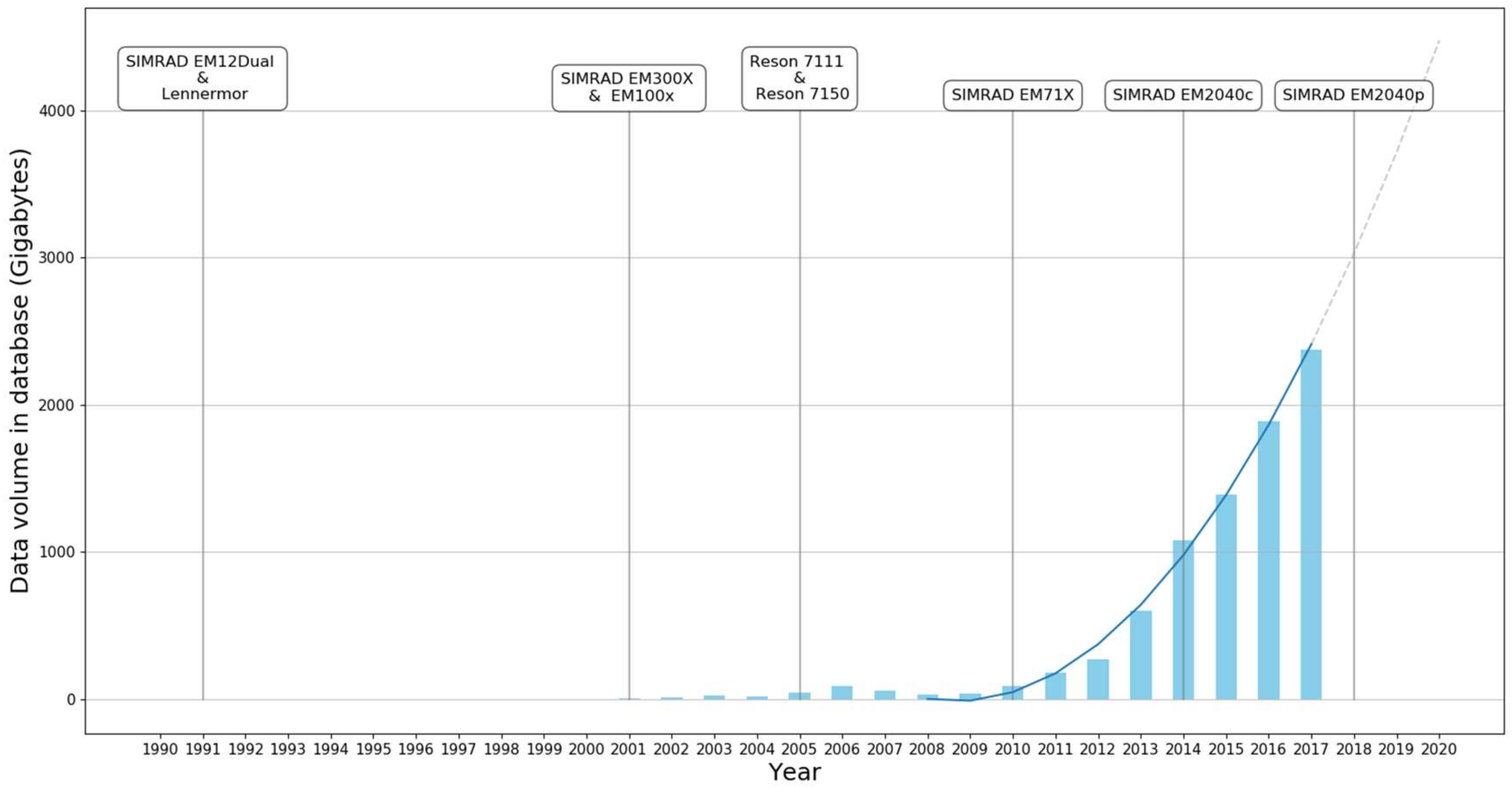
Figure 1. Volume of post-processed bathymetric data at Shom between 1991 and 2017. The last three years are missing due to the time required to integrate MBES data in the bathymetric database.
Geosciences 10 00254 g001
Figure 2. Multibeam echosounder acquisition geometry. Soundings can be described in either swath or geographic modes. In hydrography, the z-axis convention is positive down.
Geosciences 10 00254 g002
Figure 3. Bathymetric workflow.
Geosciences 10 00254 g003
Figure 4. The three types of errors depicted through a bathymetric subset. Soundings are colored according to swath lines. Bathymetric data were acquired during a boresight calibration survey in Brest harbor using a Kongsberg/SIMRAD EM2040C MBES.
Geosciences 10 00254 g004
Figure 5. Four examples of outlier’s geometries presented from the simplest to the most complex case in a navigation safety context. Soundings are colored according to depth for cases (a) to (c) and to survey line for case (d). Case (a) is the simplest case, as erroneous soundings are located below the seabed. There is no risk in deleting these soundings, as they do not represent an obstruction. Erroneous soundings located above the seabed (cases b to d) raise more issues as they potentially represent real bathymetric features. Nevertheless, in case b, isolated soundings located far from the flat seabed can be invalidated as they belong to the same swath. Case c depicts a group of soundings containing a larger number of samples. Although, being connected to the seafloor, these soundings can be invalidated as they belong to the same ping. Case (d) is the worst case to process. In this relatively noisy dataset, acquired on a shallow and rough seafloor, particular care must be taken to ensure that the shoal soundings describing the bathymetric features are preserved.
Geosciences 10 00254 g005
Figure 6. Taxonomy of outlier detection techniques in the hydrographic framework. Approaches describing several algorithms within the same class (data-oriented or surface-oriented) only appear once. * Li and Sedaghat approaches use singlebeam opportunity data.
Geosciences 10 00254 g006
Figure 7. Timeline of the different approaches.
Geosciences 10 00254 g007
Figure 8. Number of citations per algorithm (as extracted from Google Scholar 30/01/2020).
Geosciences 10 00254 g008
Figure 9. (a) Type of data representation per article; (b) type of dataset per method; (c) type of metrics performance used for each article; (d) output information given by the algorithms.
Geosciences 10 00254 g009
Table 1. Examples of survey on Shom’s reference areas.
YearMBESArea 1Number of SoundingsAngular SectorCovered Area
2012EM3002CR2,608,853150° maximum0.100 km2
2017EM1002PN693,417150° maximum3.270 km2
2019EM2040cCR4,376,801150° maximum0.104 km2
2016EM710PN7,160,800150° maximum2.753 km2
2020EM712PN6,455,200150° maximum3.227 km2
1: These reference areas are known as CR: Carré Renard 20 m mean depth, PN: Pierres Noires 60 m mean depth.
Table 2. Characteristics of data-oriented.
ApproachClass 1Overall
Structure 2
Description
Mode 3
Neighborhood 4Techniques 5
[2] GuentherS1TFaStatistical filter: mean, multiple of standard deviation on windows of 3 beams × 5 pings
[48] HerlihyS3 CTFau(1)
  • Depth or cross track distance (3);
  • Non-zero neighboring (1);
  • Statistical filter: Weighted average of neighboring soundings (4);
[50] WareS1SFu(1)Classification of soundings according into 8 classes based on a linear combination of weighted average and standard deviation Weighted average, applied to each cell of a base surface (3)
[35] EegS1SFau(1)Inspection of a reduced list of soundings sorted by a quotient (i.e., outlierness score) (1).
[49] BourilletS4 CBFau(1)
  • Distribution of depths in a ping (user defined thresholds);
  • Difference of mean values between pings computed in 3 × 3 boxes (1);
  • Slope variation between 3 beams (2);
  • Sounding filter based on bilinear interpolation computed from a DBM built by averaging soundings belonging to a cell (1);
[27] DuC3 CTFau(2)
  • Depth gate (2)
  • Outliers histogram modes clustering embedded in a coarse-to-fine data scan: group of pings subdivided into across-track working window (2);
  • Dixon discordance test
[30] BisquayS2 SSFu(3)
  • Depth increments method (2);
  • Quantile method (4)
[46] LirakisS5 CBFau(1)
  • Depth gate (2);
  • Tolerance values estimated per beam using a boostrap procedure initiated from pivot ping (2);
  • Validation of data belonging to the mode of 2D histogram (2);
  • Validation of soundings based on local extremal values (0)
  • Invalidation according to standard deviation value (0)
[31] HouS3 CTFau(1)
  • Statistical filter based on Global/local variance criteria (2);
  • Statistical filter based on two sample variances (0);
  • Bad ping detection (1);
[16] KammererC4 SBFau(1)
  • Histogram segmentation (2 *);
  • Entropy segmentation (0 *);
  • Fuzzy k mean segmentation (1 *);
  • Mosaic segmentation (0 *);
[38] MannS1SFu(1)Statistical filter based on median (1);
[17] CalderS1SFu(2)CUBE (4 *);
[33] BottelierS2 STFa
0.
Depth Gate (2);
1.
1D cross validation (1);
2.
2D cross validation (1);
[32] YangDe2 CTFu(1)
  • Region growing from dense bins by applying morphological operations (2);
  • Edge tracing to ascertain outer edge (1);
  • Statistical filter based on median (1);
[4] CalderS1SFu(4)CHRT (4 *);
[42] ArgeDi1SFaConnected-component of a TIN after edges removing (1);
[47] SedaghatDe/C2 SSFu(1)Combination of LOF and DBSCAN algorithms to find spatio-temporal clusters (3);
Hotspot detection from local Moran’I and z-score statistics (1);
[51] FerreiraS3 SSFau(1)
0.
Exploratory data statistical analysis to control the spatial independence of data and variogram analysis user (1 *)
1.
Adjusted boxplot (0);
2.
Modified Z-score (0);
3.
δ method (1);
[39] LiS2 CSFa
  • Statistical filter based on median (1)
  • minimum value (1);
1 Class of approach: S: stochastic; De: density; Di: distance; C: clustering; 2 the number of techniques developed by the approach. When the number of techniques is greater than 1, the retained structure is detailed: C means that techniques are applied in cascade, S: separately; 3 input data are described in T: temporal mode; S: spatial mode; B: both modes; 4 neighborhood is: Fa: fixed by the approach; Fu(x): fixed by the user using x parameters; Fau(x): fixed by both the approach and the user using x parameters; 5 the number in parentheses indicates the number of parameters of the technique. *: hidden parameters exist but are not explicitly mentioned in the paper.
Table 3. Characteristics of surface-oriented algorithms.
AlgorithmDescription Mode 1Observation Type 2Approach Scope 3Robust Estimation 4Approach Type. In the Case of a Robust Estimation Approach, Type of the Robust EstimatorInitial Step 5Surface Type
[34] ArnoldSAL0Graduated Non-convexity algorithm0Weak membrane (first order)/Thin plate (second order)
[34] ArnoldSPL1Robust linear prediction involved in an auto-regressive process0First-order non symmetric half-plane (NSHP) image model/bidirectional vector
[30] BisquaySPL0 1Ordinary kriging—Linear variogram
[41] MotaoGPG1IGIII (M-Estimator)1IDW
[28] CanepaGPG1Tukey (M-Estimator)1Local polynomial
[33] BottelierGAG1M-estimator0Ordinary kriging—Gaussian model
[37] BjorkeBAG0-0Biquadratic polynomial
[40] LuBAL1LTS estimator0Second/third order polynomial
[25] DebeseBAL1Tukey (M-Estimator)1Polynomial
[53] RezvaniGAL1Huber; IGGIII, Hampel, Tukey (M-estimator)1Horizontal plane
[18] LadnerGAL1LTS estimator0Polynomial
[52] WangBAG1Huber (M-Estimator)1Improved Multi Quadric model
[26] WangBAG1IGIII (M-Estimator)1Multi Quadric model
[29] HuangGAG0Sparse weighted LS-SVM Polynomial and gauss radial kernel function
1 Input data are described in T: temporal mode; S: spatial mode; B: both modes; 2 observed from a P: point-based; A: area-based; approach; 3 scope of the approach from G: global; L: local; 4 robust estimation approach 0: No; 1: Yes; 5 initial step required 0: No; 1: Yes.
Table 4. Characteristics of real testing datasets.
AlgorithmDepth Range 1Sensor ModelDatasets
Number ofVolumeType 2
[2] GuentherD/VDBS 3---
[48] HerlihyD/VDSeabeam
Hydro Chart
223,735,009; 15,622,682-
[50] Ware-Navitronics 31200,000A
[34] Arnold-MBES 41-P
[35] EegSMBES 4165,000S
[49] BourilletD/VDSIMRAD EM12D; EM1000---
[27] DuSSIMRAD EM10001--
[30] BisquayVDSIMRAD EM12D346,592; 108,297; 189,699S
[41] Motao-Chinese-developed H/HCS-0171198,928A
[3] DebeseS/D/VDSIMRAD EM12D EM3000 Lennermor538,000; 46,000;
88,000; 108,000;
178,000
S
[46] LirakisSSIMRAD EM1000 EM3000 EM1215774,400;
300,800;
665,600;
1,251,200; 195,200
A
[16] KammererSSIMRAD EM1002S Atlas FS202-A
[56] DebeseS/D/VDSIMRAD EM12D EM30003108,000; 178,000;
195,200
S
[31] HouSSAX-99 (Destin FL)-6.9 Go 5A
[38] MannSSIMRAD EM30001641,421A
[28] CanepaS/DSIMRAD EM3000 HYDROSWEEP MD336,482;
1,220,358;
500,000
A
[17] CalderS/DSIMRAD EM3000
SIMRAD EM1002
21,000,153A
[33] BottelierSReson8101 mounted on a ROV1300,000S
[54] DebeseS/DATLAS Fansweep20 SIMRAD EM3000 EM1002, EM1204550,000 to
3,000,000
A
[32] YangVD-1(9.6 × 30.2) km2 6S
[39] LiSSDH-13D 71619S
[37] BjorkeSSIMRAD EM1002193,424A
[40] LuS-16,350P
[42] Arge-MBES (4)37,000,000;
7,000,000;
6,000,000
A
[55] HuangSReson 8101113,300A
[4] CalderS-1100 m × 200 m 8A
[25] DebeseSSIMRAD EM300212,600,000A
[47] SedaghatSSBES 911,500,000A
[53] RezvaniSAtlas Fansweep 20132,020S
[18] LadnerD/VD-24,318,703;
260,527
A
[52] WangSMBES 411045P
[26] WangSMBES 411904P
[29] HuangVDSeabeam 211216268S
[51] FerreiraSR2Sonic 202218090S
1: Depth ranges are labeled using: S for shallow, D for deep and VD for very deep; 2: type of datasets are labeled using A: for area, S: swath line; P: group of pings; 3: sweep system; 4: no other information provided; 5: Hou provides the volume of data in gigabytes; 6: Yang does not provide a volume but the covered surface of the survey; 7: an SBES system; 8: DBM’s size; 9: Crowdsourced data.