A Probabilistic Assessment of Soil Erosion Susceptibility in a Head Catchment of the Jemma Basin, Ethiopian Highlands


 ,
,  and
and 
Abstract
1. Introduction
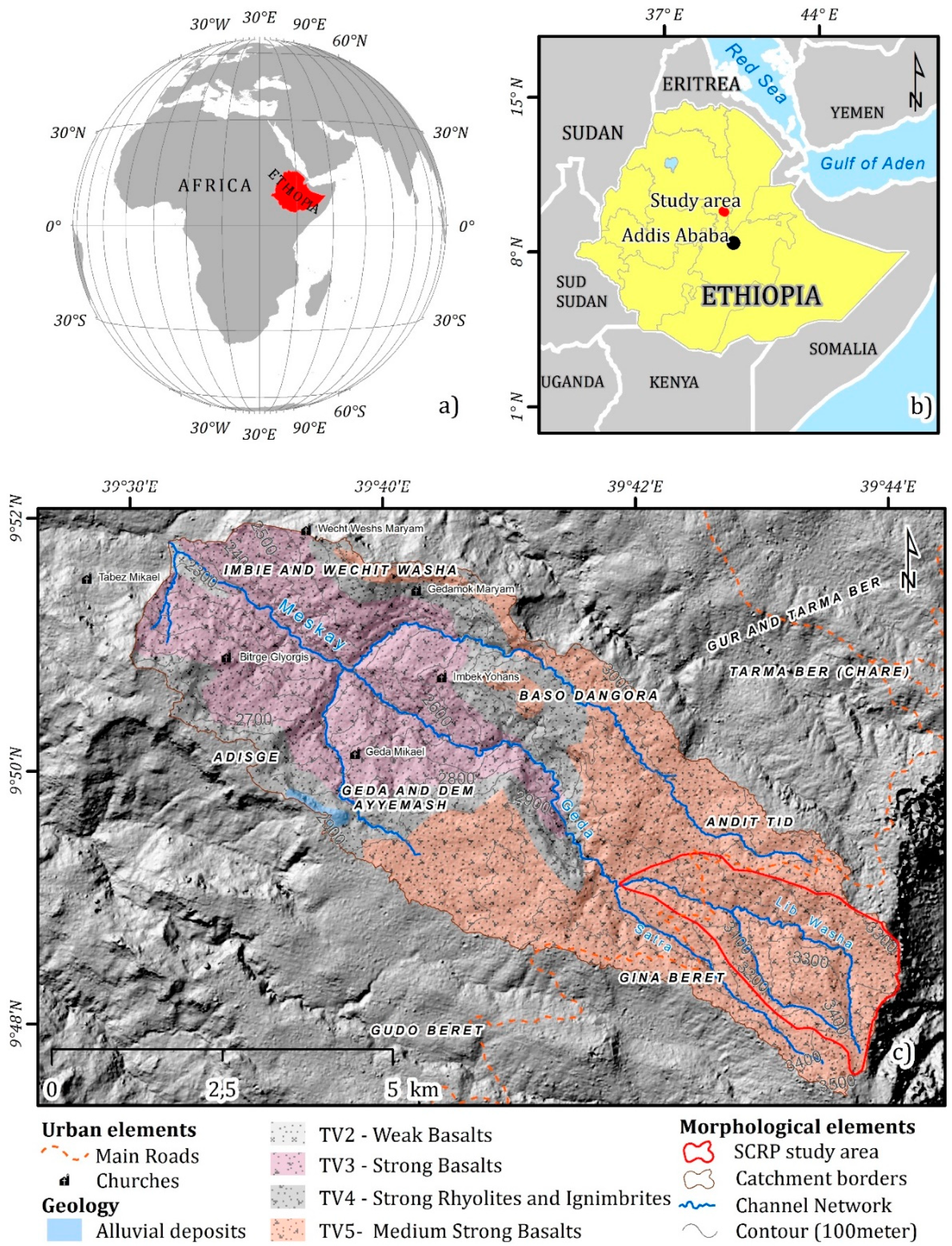
2. Regional Setting
3. Materials and Methods
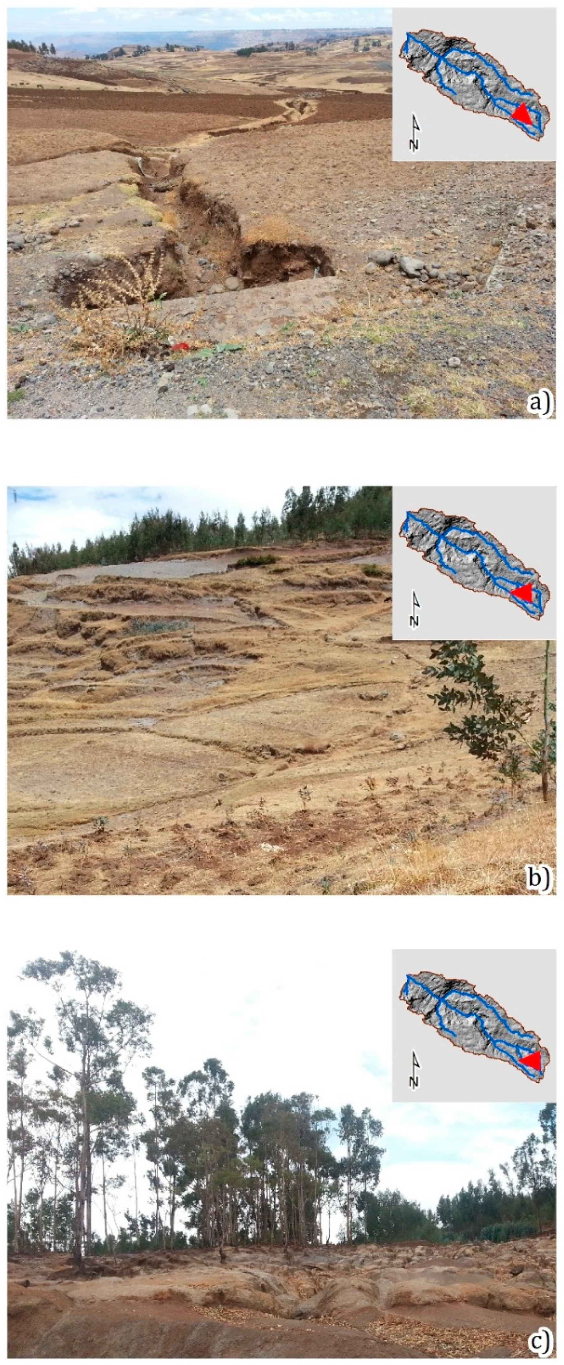
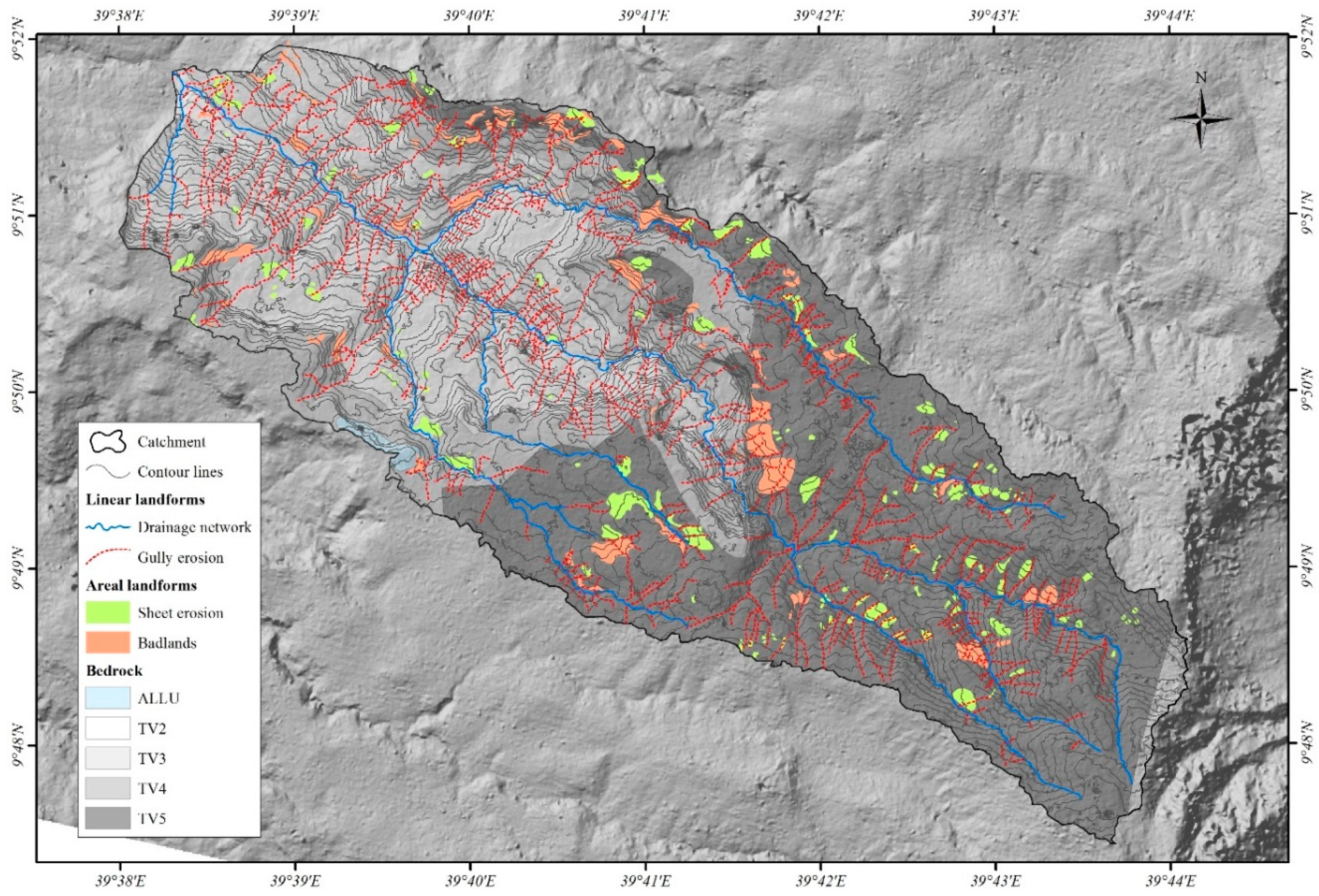
3.1. Geomorphological Mapping
3.2. Explanatory Variables
3.2.1. Remotely Sensed Data
3.2.2. Topographic Indices
3.3. Predictive Modeling Approach
3.4. Model Evaluation
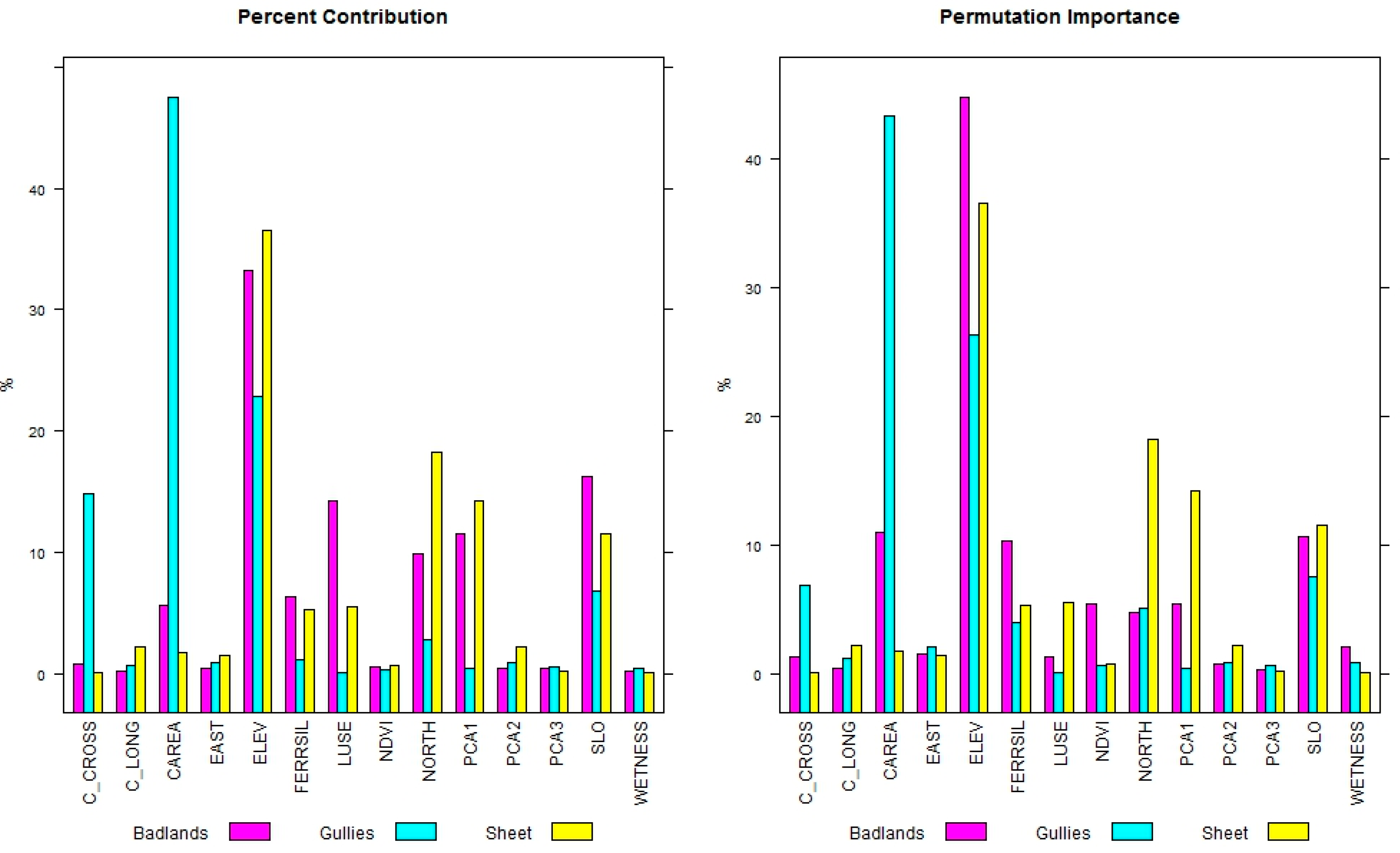
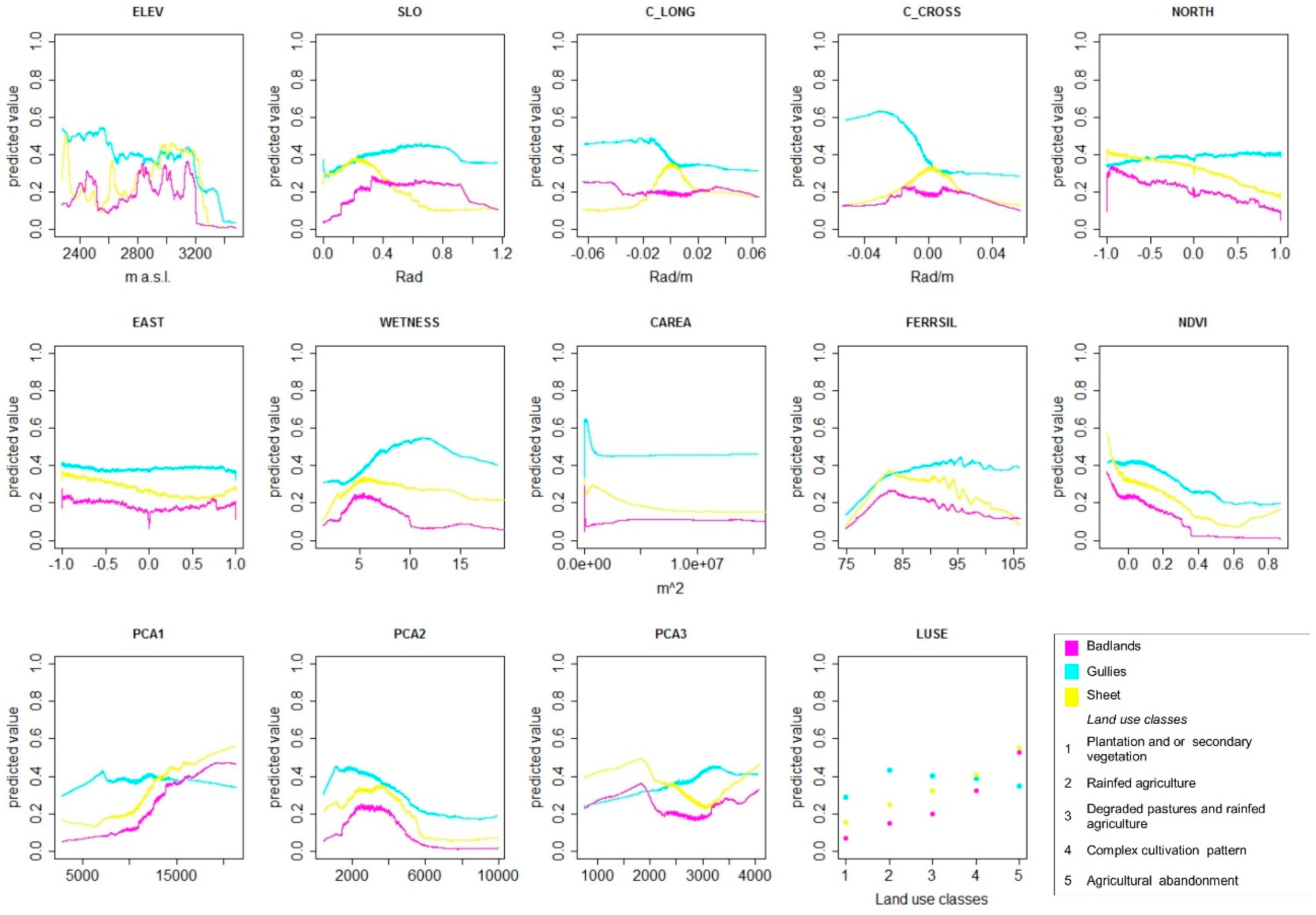
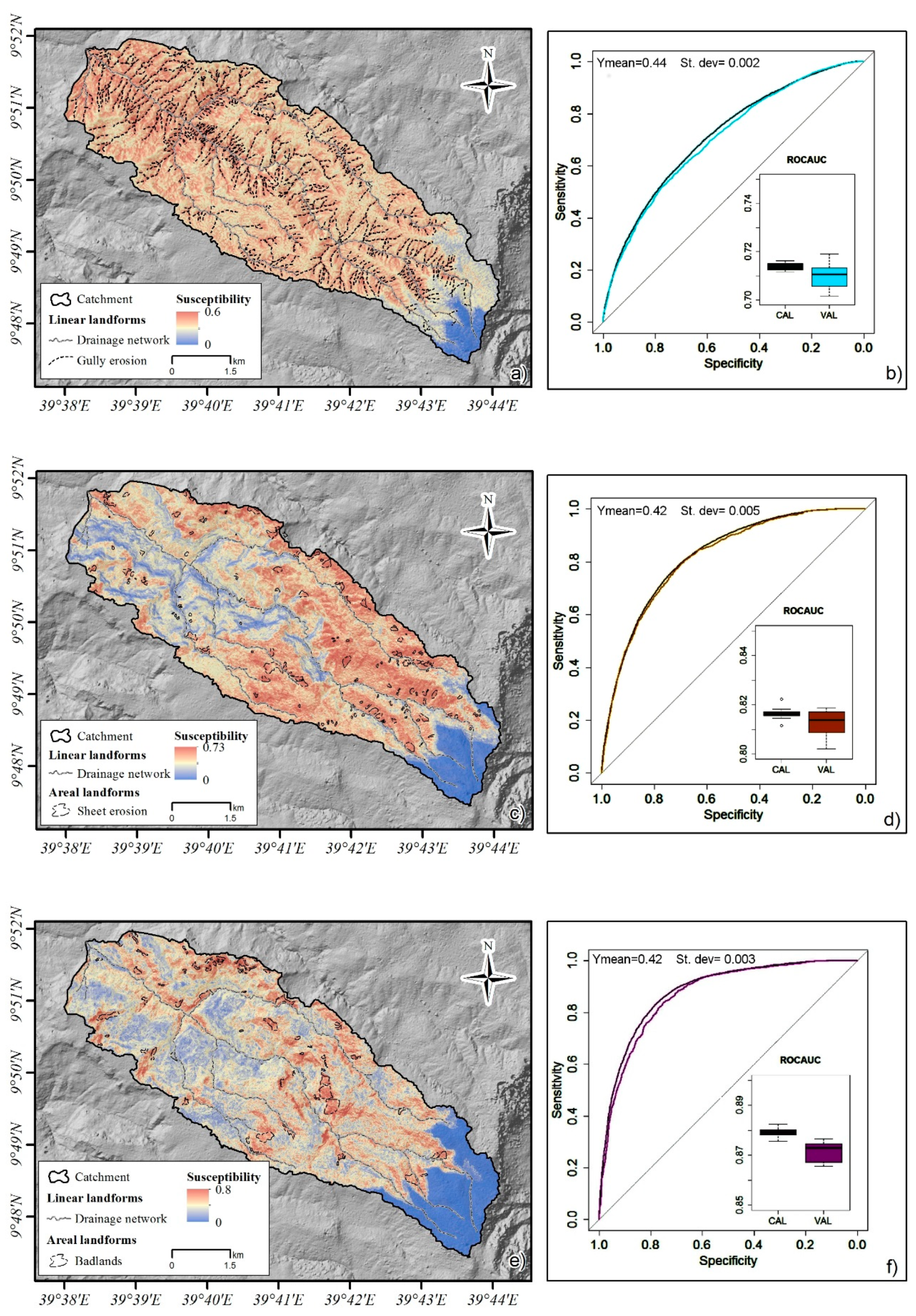
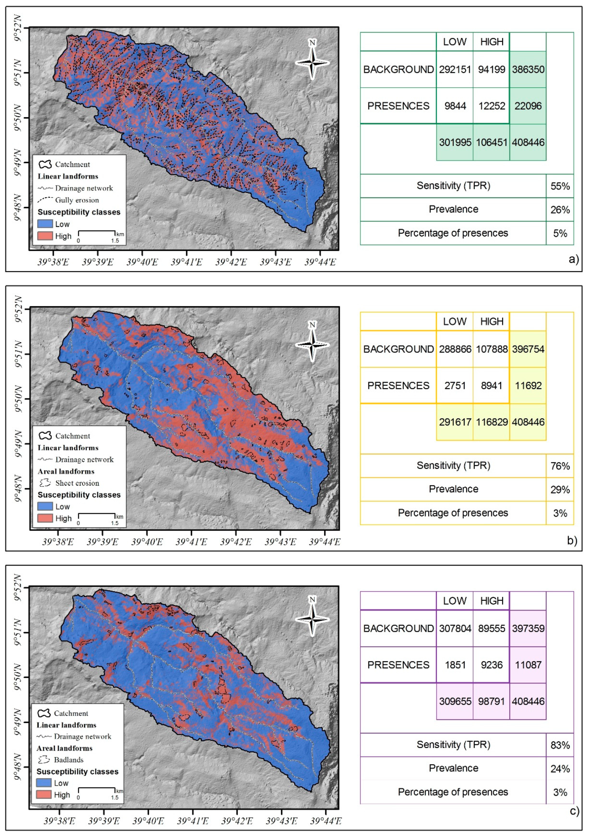
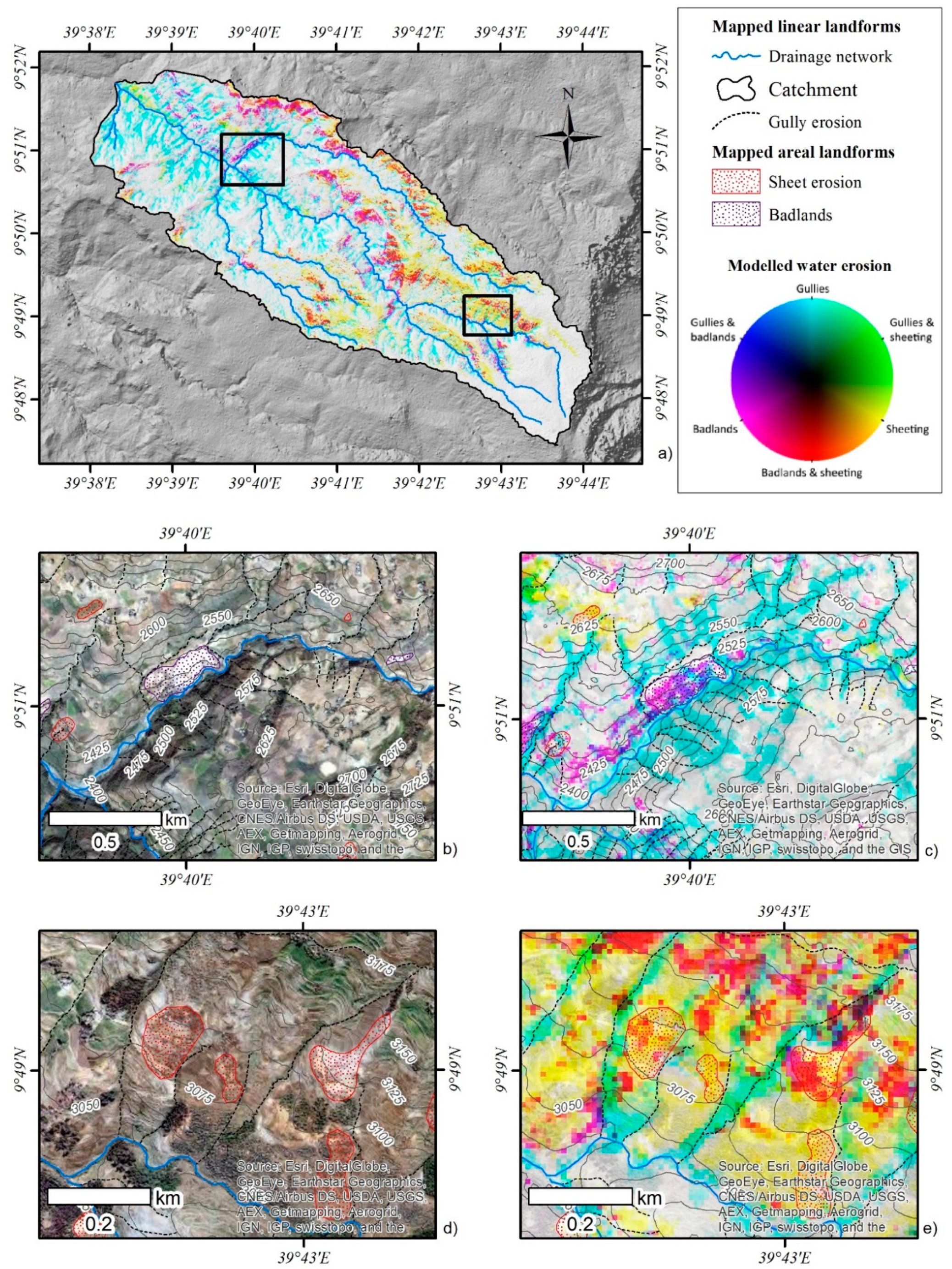
4. Results
5. Discussion
6. Conclusions
Author Contributions
Funding
Acknowledgments
Conflicts of Interest
References
- Bosino, A.; Omran, A.; Märker, M. Identification, characterisation and analysis of the Oltrepo Pavese calanchi in the Northern Apennines (Italy). Geomorphology 2019, 340, 53–66. [Google Scholar] [CrossRef]
- Tamene, L.; Vlek, P.L.G. Soil Erosion Studies in Northern Ethiopia. In Land Use and Soil Resources; Braimoh, A.K., Vlek, P.L.G., Eds.; Springer: Dordrecht, The Netherlands, 2008; pp. 73–100. ISBN 978-1-4020-6778-5. [Google Scholar]
- Nyssen, J.; Poesen, J.; Haregeweyn, N.; Parsons, T. Environmental change, geomorphic processes and land degradation in tropical highlands. Catena 2008, 75, 1–4. [Google Scholar] [CrossRef]
- Kusák, M.; Kropáček, J.; Vilímek, V.; Scillaci, C. Analysis of the influence of tectonics on the evolution of valley networks based on SRTM DEM, Jemma River basin, Ethiopia. Geogr. Fis. Din. Quat. 2016, 1, 37–50. [Google Scholar] [CrossRef]
- Kropacek, J.; Vařilová, Z.; Baroň, I.; Bhattacharya, A.; Eberle, J.; Hochschild, V. Remote Sensing for Characterisation and Kinematic Analysis of Large Slope Failures: Debre Sina Landslide, Main Ethiopian Rift Escarpment. Remote Sens. 2015, 7, 16183–16203. [Google Scholar] [CrossRef]
- Merritt, W.; Letcher, R.; Jakeman, A.J. A review of erosion and sediment transport models. Environ. Model. Softw. 2003, 18, 761–799. [Google Scholar] [CrossRef]
- Montgomery, D.R.; Dietrich, W.E.; Bonfini, L.; Karlovich, C.; Dasgupta, C.; Banerjee, U. Channel Initiation and the Problem of Landscape Scale. Science 1992, 255, 826–830. [Google Scholar] [CrossRef]
- Samani, A.N.; Ahmadi, H.; Jafari, M.; Boggs, G.; Ghoddousi, J.; Malekian, A. Geomorphic threshold conditions for gully erosion in Southwestern Iran (Boushehr-Samal watershed). J. Asian Earth Sci. 2009, 35, 180–189. [Google Scholar] [CrossRef]
- Beck, M.B. Water quality modeling: A review of the analysis of uncertainty. Water Resour. Res. 1987, 23, 1393–1442. [Google Scholar] [CrossRef]
- Wheater, H.S.; Jakeman, A.J.; Beven, K.J. Progress and directions in rainfall-runoff modelling. In Modelling Change in Environmental Systems; Wiley: Chichester, UK, 1993; pp. 101–132. ISBN 0-471-94263-4. [Google Scholar]
- Sorooshian, S. Parameter Estimation, Model Identification, and Model Validation: Conceptual-Type Models. In Recent Advances in the Modeling of Hydrologic Systems; Bowles, D.S., O’Connell, P.E., Eds.; Springer: Dordrecht, The Netherlands, 1991; pp. 443–467. ISBN 978-94-011-3480-4. [Google Scholar]
- Beven, K. How to make advances in hydrological modelling. Hydrol. Res. 2019, 50, 1481–1494. [Google Scholar] [CrossRef]
- Singh, V.P. Hydrologic modeling: Progress and future directions. Geosci. Lett. 2018, 5, 15. [Google Scholar] [CrossRef]
- Botero-Acosta, A.; Chu, M.L.; Guzman, J.A.; Starks, P.J.; Moriasi, D.N. Riparian erosion vulnerability model based on environmental features. J. Environ. Manag. 2017, 203, 592–602. [Google Scholar] [CrossRef] [PubMed]
- Atkinson, P.M.; Massari, R. Generalised linear modelling of susceptibility to landsliding in the central Apennines, Italy. Comput. Geosci. 1998, 24, 373–385. [Google Scholar] [CrossRef]
- Cama, M.; Lombardo, L.; Conoscenti, C.; Agnesi, V.; Rotigliano, E. Predicting storm-triggered debris flow events: Application to the 2009 Ionian Peloritan disaster (Sicily, Italy). Nat. Hazards Earth Syst. Sci. 2015, 15, 1785–1806. [Google Scholar] [CrossRef]
- Cama, M.; Conoscenti, C.; Lombardo, L.; Rotigliano, E. Exploring relationships between grid cell size and accuracy for debris-flow susceptibility models: A test in the Giampilieri catchment (Sicily, Italy). Environ. Earth Sci. 2016, 75, 1–21. [Google Scholar] [CrossRef]
- Goetz, J.; Brenning, A.; Petschko, H.; Leopold, P. Evaluating machine learning and statistical prediction techniques for landslide susceptibility modeling. Comput. Geosci. 2015, 81, 1–11. [Google Scholar] [CrossRef]
- Rossi, M.; Guzzetti, F.; Reichenbach, P.; Mondini, A.C.; Peruccacci, S. Optimal landslide susceptibility zonation based on multiple forecasts. Geomorphology 2010, 114, 129–142. [Google Scholar] [CrossRef]
- Conoscenti, C.; Rotigliano, E.; Cama, M.; Arias, N.A.C.; Lombardo, L.; Agnesi, V. Exploring the effect of absence selection on landslide susceptibility models: A case study in Sicily, Italy. Geomorphology 2016, 261, 222–235. [Google Scholar] [CrossRef]
- Gutiérrez, A.G.; Conoscenti, C.; Angileri, S.E.; Rotigliano, E.; Schnabel, S. Using topographical attributes to evaluate gully erosion proneness (susceptibility) in two mediterranean basins: Advantages and limitations. Nat. Hazards 2015, 79, 291–314. [Google Scholar] [CrossRef]
- Märker, M.; Pelacani, S.; Schröder, B.; Märker, M. A functional entity approach to predict soil erosion processes in a small Plio-Pleistocene Mediterranean catchment in Northern Chianti, Italy. Geomorphology 2011, 125, 530–540. [Google Scholar] [CrossRef]
- Gutiérrez, A.G.; Schnabel, S.; Contador, F.L. Using and comparing two nonparametric methods (CART and MARS) to model the potential distribution of gullies. Ecol. Model. 2009, 220, 3630–3637. [Google Scholar] [CrossRef]
- Veronesi, F.; Hurni, L. Random Forest with semantic tie points for classifying landforms and creating rigorous shaded relief representations. Geomorphology 2014, 224, 152–160. [Google Scholar] [CrossRef]
- Angileri, S.E.; Conoscenti, C.; Hochschild, V.; Märker, M.; Rotigliano, E.; Agnesi, V.; Märker, M. Water erosion susceptibility mapping by applying Stochastic Gradient Treeboost to the Imera Meridionale River Basin (Sicily, Italy). Geomorphology 2016, 262, 61–76. [Google Scholar] [CrossRef]
- Schillaci, C.; Lombardo, L.; Saia, S.; Fantappiè, M.; Märker, M.; Acutis, M. Modelling the topsoil carbon stock of agricultural lands with the Stochastic Gradient Treeboost in a semi-arid Mediterranean region. Geoderma 2017, 286, 35–45. [Google Scholar] [CrossRef]
- Lombardo, L.; Cama, M.; Conoscenti, C.; Marker, M.; Rotigliano, E. Binary logistic regression versus stochastic gradient boosted decision trees in assessing landslide susceptibility for multiple-occurring landslide events: Application to the 2009 storm event in Messina (Sicily, southern Italy). Nat. Hazards 2015, 79, 1621–1648. [Google Scholar] [CrossRef]
- Lombardo, L.; Bachofer, F.; Cama, M.; Märker, M.; Rotigliano, E. Exploiting Maximum Entropy method and ASTER data for assessing debris flow and debris slide susceptibility for the Giampilieri catchment (north-eastern Sicily, Italy). Earth Surf. Process. Landf. 2016, 41, 1776–1789. [Google Scholar] [CrossRef]
- Zakerinejad, R.; Märker, M. Prediction of gully erosion susceptibility using detailed terrain analysis and Maximum Entropy Modeling: A case study in the Mazayejan plain, Southwest Iran. Geogr. Fis. Din. Quat. 2014, 37, 1–10. [Google Scholar] [CrossRef]
- Maerker, M.; Bosino, A.; Scopesi, C.; Giordani, P.; Firpo, M.; Rellini, I. Assessment of calanchi and rill-interrill erosion susceptibility in northern Liguria, Italy: A case study using a probabilistic modelling framework. Geoderma 2020, 371, 114367. [Google Scholar] [CrossRef]
- Hjort, J.; Ujanen, J.; Parviainen, M.; Tolgensbakk, J.; Etzelmüller, B. Transferability of geomorphological distribution models: Evaluation using solifluction features in subarctic and Arctic regions. Geomorphology 2014, 204, 165–176. [Google Scholar] [CrossRef]
- Tilahun, S.A.; Guzman, C.D.; Zegeye, A.D.; Engda, T.A.; Collick, A.S.; Rimmer, A.; Steenhuis, T.S. An efficient semi-distributed hillslope erosion model for the subhumid Ethiopian Highlands. Hydrol. Earth Syst. Sci. 2013, 17, 1051–1063. [Google Scholar] [CrossRef]
- Steenhuis, T.S.; Collick, A.S.; Easton, Z.M.; Leggesse, E.S.; Bayabil, H.K.; White, E.; Awulachew, S.B.; Adgo, E.; Ahmed, A.A. Predicting discharge and sediment for the Abay (Blue Nile) with a simple model. Hydrol. Process. 2009, 23, 3728–3737. [Google Scholar] [CrossRef]
- Haregeweyn, N.; Poesen, J.; Verstraeten, G.; Govers, G.; De Vente, J.; Nyssen, J.; Deckers, J.; Moeyersons, J. Assessing the performance of a spatially distributed soil erosion and sediment delivery model (watem/sedem) in northern ethiopia. Land Degrad. Dev. 2011, 24, 188–204. [Google Scholar] [CrossRef]
- Nyssen, J.; Poesen, J.; Moeyersons, J.; Haile, M.; Deckers, J. Dynamics of soil erosion rates and controlling factors in the Northern Ethiopian Highlands—Towards a sediment budget. Earth Surf. Process. Landf. 2008, 33, 695–711. [Google Scholar] [CrossRef]
- Sima, J. Water Resources Management and Nvironmental Protection Studies of the Jemma Basin River for Improved Food Security; AcquaTest: White Lake, MI, USA, 2009. [Google Scholar]
- Kropáček, J.; Schillaci, C.; Salvini, R.; Märker, M. GFDQ—Geografia Fisica e Dinamica Quaternaria 039_2_06_2016. Geogr. Fis. Dinam. Quat. 2016, 39, 161–170. [Google Scholar] [CrossRef]
- Frankl, A.; Stal, C.; Abraha, A.; Nyssen, J.; Rieke-Zapp, D.; De Wulf, A.; Jean, P. Detailed recording of gully morphology in 3D through image-based modelling. Catena 2015, 127, 92–101. [Google Scholar] [CrossRef]
- Märker, M.; Hochschild, V.; Maca, V.; Vilímek, V. Stochastic assessment of landslides and debris flows in the Jemma Basin, Blue Nile, Central Ethiopia. Geogr. Fis. Din. Quat. 2016, 39, 51–58. [Google Scholar]
- Phillips, S.J.; Anderson, R.P.; Schapire, R.E. Maximum entropy modeling of species geographic distributions. Ecol. Model. 2006, 190, 231–259. [Google Scholar] [CrossRef]
- Elith, J.; Graham, C.H.; Anderson, R.P.; Dudík, M.; Ferrier, S.; Guisan, A.; Hijmans, R.J.; Huettmann, F.; Leathwick, J.R.; Lehmann, A.; et al. Novel methods improve prediction of species’ distributions from occurrence data. Ecography 2006, 29, 129–151. [Google Scholar] [CrossRef]
- Maerker, M.; Schillaci, C.; Melis, R.T.; Kropáček, J.; Bosino, A.; Vilímek, V.; Hochschild, V.; Sommer, C.; Altamura, F.; Mussi, M. Geomorphological processes, forms and features in the surroundings of the Melka Kunture Palaeolithic site, Ethiopia. J. Maps 2019, 15, 797–806. [Google Scholar] [CrossRef]
- Bachofer, F.; Quénéhervé, G.; Hochschild, V.; Maerker, M. Multisensoral Topsoil Mapping in the Semiarid Lake Manyara Region, Northern Tanzania. Remote Sens. 2015, 7, 9563–9586. [Google Scholar] [CrossRef]
- Spyromitros-Xioufis, E.; Groves, W. Multi-Label Classification Methods for Multi-Target Regression. arXiv 2012, arXiv:1211.6581. [Google Scholar]
- Lombardo, L.; Fubelli, G.; Amato, G.; Bonasera, M. Presence-only approach to assess landslide triggering-thickness susceptibility: A test for the Mili catchment (north-eastern Sicily, Italy). Nat. Hazards 2016, 84, 565–588. [Google Scholar] [CrossRef]
- Hurni, G. Land Degradation, Famines and Resource Scenarios in Ethiopia. In. World Soil Erosion and Conservation; Pimentel, D., Ed.; Cambridge University Press: Cambridge, UK, 1993; pp. 27–62. [Google Scholar]
- Shiferaw, B. Resource degradation and adoption of land conservation technologies in the Ethiopian Highlands: A case study in Andit Tid, North Shewa. Agric. Econ. 1998, 18, 233–247. [Google Scholar] [CrossRef]
- Zanettine, B.; Justine-Visentine, E.; Piccirillo, E.M. Volcanic Succession, Tectonics and Magmatologyin Central Ethiopia; Istituto di Mineralogia e Petrologia, Universitá degli Studi di Padova: Padua, Italy, 1978. [Google Scholar]
- Haregeweyn, N.; Tsunekawa, A.; Nyssen, J.; Poesen, J.; Tsubo, M.; Meshesha, D.T.; Schütt, B.; Adgo, E.; Tegegne, F. Soil erosion and conservation in Ethiopia. Prog. Phys. Geogr. Earth Environ. 2015, 39, 750–774. [Google Scholar] [CrossRef]
- Engda, T.A. Modeling Rainfall, Runoff and Soil Loss Relationships in the Northeastern Highlands of Ethiopia, Andit Tid Watershed. Ph.D. Thesis, Cornell University, Ithaca, NY, USA, August 2009. [Google Scholar]
- Yitaferu, B.; Abewa, A.; Amare, T. Expansion of Eucalyptus Woodlots in the Fertile Soils of the Highlands of Ethiopia: Could It Be a Treat on Future Cropland Use? J. Agric. Sci. 2013, 5, 97. [Google Scholar] [CrossRef]
- Hurni, H. Area of Andit Tid, Shewa, Ethiopia: Long-Term Monitoring of the Agricultural Environment 1982–1994; SCRP (Soil Conservation Research Programme): Shewa, Ethiopia, 2000. [Google Scholar]
- Liu, B.M.; Collick, A.S.; Zeleke, G.; Adgo, E.; Easton, M.Z.; Steenhuis, T.S. Rainfall-discharge relationships for a monsoonal climate in the Ethiopian highlands. Hydrol. Process. 2008, 2274, 2267–2274. [Google Scholar] [CrossRef]
- Herweg, K.; Ludi, E. The performance of selected soil and water conservation measures—case studies from Ethiopia and Eritrea. Catena 1999, 36, 99–114. [Google Scholar] [CrossRef]
- Tezera, A.; Chanie, T.; Feyisa, T.; Jemal, A. Impact Assessment of Land Use/ Land Cover Change on Soil Erosion and Rural Livelihood in Andit Tid Watershed, North Shewa, Ethiopia. Arch. Curr. Res. Int. 2016, 3, 1–10. [Google Scholar] [CrossRef]
- Fiorucci, F.; Ardizzone, F.; Rossi, M.; Torri, D. The use of stereoscopic satellite images to map rills and ephemeral gullies. Remote Sens. 2015, 7, 14151–14178. [Google Scholar] [CrossRef]
- Guzzetti, F.; Mondini, A.C.; Cardinali, M.; Fiorucci, F.; Santangelo, M.; Chang, K.T. Landslide inventory maps: New tools for an old problem. Earth-Sci. Rev. 2012, 112, 42–66. [Google Scholar] [CrossRef]
- Auerswald, K.; Schmidt, F. Atlas der Erosionsgefährdung in Bayern--Karten zum flächenhaften Bodenabtrag durch Regen.--GLA-Fachberichte 1; Bayer. Geol. Landesamt (Hrsg.): München, Germany, 1986. [Google Scholar]
- Selby, M.J. Hillslope Materials and Processes, 2nd ed.; Oxford University Press: Oxford, UK, 1993; ISBN 9780198741831. [Google Scholar]
- Hutchinson, D.E.; Pritchard, H.W. Resource conservation glossary. J. Soil Water Conserv. 1976, 31, 1–63. [Google Scholar]
- Higgins, C.G.; Coates, D.R. (Eds.) Groundwater Geomorphology: The Role of Subsurface Water in Earth-surface Processes and Landforms; Geological Society of America: Boulder, CO, USA, 1990; Volume 252. [Google Scholar]
- Fairbridge, R.W. The Encyclopedia of Geomorphology. Rhodes W. Fairbridge, Ed. Reinhold, New York, 1968. xvi + 1296 pp.,. Encyclopedia of Earth Sciences Series, vol. 3. Science (80-. ) 1969, 165, 53. [Google Scholar] [CrossRef]
- Howard, A.D. Badland Morphology and Evolution: Interpretation Using a Simulation Model. Earth Surf. Process. Landforms 1997, 22, 211–227. [Google Scholar] [CrossRef]
- Dickinson, A.; Collins, R. Predicting erosion and sediment yield at the catchment scale. In Soil Erosion at Multiple Scales: Principles and Methods for Assessing Causes and Impacts; CABI: Wallingford, UK, 1998; pp. 317–342. [Google Scholar]
- Mondini, A.C.; Guzzetti, F.; Reichenbach, P.; Rossi, M.; Cardinali, M.; Ardizzone, F. Remote Sensing of Environment Semi-automatic recognition and mapping of rainfall induced shallow landslides using optical satellite images. Remote Sens. Environ. 2011, 115, 1743–1757. [Google Scholar] [CrossRef]
- Martha, T.R.; Kerle, N.; Jetten, V.; Van Westen, C.J.; Kumar, K.V. Geomorphology Characterising spectral, spatial and morphometric properties of landslides for semi-automatic detection using object-oriented methods. Geomorphology 2010, 116, 24–36. [Google Scholar] [CrossRef]
- Curzio, S.L.; Magliulo, P. Soil erosion assessment using geomorphological remote sensing techniques: An example from Southern Italy. Earth Surf. Process. Landf. 2010, 35, 262–271. [Google Scholar] [CrossRef]
- Alatorre, L.C.; Beguería, S. Identification of eroded areas using remote sensing in a badlands landscape on marls in the central Spanish Pyrenees. Catena 2009, 76, 182–190. [Google Scholar] [CrossRef]
- Desprats, J.F.; Raclot, D.; Rousseau, M.; Cerdan, O.; Garcin, M.; Le Bissonnais, Y.; Ben Slimane, A.; Fouche, J.; Monfort-Climent, D. Mapping Linear Erosion Features Using High And Very High Resolution Satellite Imagery. L. Degrad. Dev. 2013, 24, 22–32. [Google Scholar] [CrossRef]
- Otto, J.-C.; Smith, M.J. Geomorphological mapping. Geomorphol. Tech. 2013, 2, 1–10. [Google Scholar] [CrossRef]
- Alexander, D. Difference between ‘Calachi’ and ‘Biancane’ Badlands in Italy. In Badland Geomorphology and Piping; Geo Abstracts: Norwich, UK, 1982; pp. 71–78. [Google Scholar]
- Cudahy, T. Satellite ASTER Geoscience Product Notes for Australia; Report Number EP-30-07-12-44. 2012. Available online: http://citeseerx.ist.psu.edu/viewdoc/download?doi=10.1.1.700.1754&rep=rep1&type=pdf (accessed on 11 May 2020).
- Tapsall, B.; Milenov, P.; Tasdemir, K. Analysis of Rapideye Imagery for Annual Landcover Mapping As an Aid To European Union ( Eu ) Common Agricultural Policy. 100 Years ISPRS - Adv. Remote Sens. Sci. 2010, XXXVIII, 568–573. [Google Scholar] [CrossRef]
- Fernández-Landa, A.; Algeet-Abarquero, N.; Fernández-Moya, J.; Guillén-Climent, M.; Pedroni, L.; García, F.; Espejo, A.; Villegas, J.F.; Marchamalo, M.; Bonatti, J.; et al. An Operational Framework for Land Cover Classification in the Context of REDD+ Mechanisms. A Case Study from Costa Rica. Remote Sens. 2016, 8, 593. [Google Scholar] [CrossRef]
- Congalton, R.G. A review of assessing the accuracy of classifications of remotely sensed data. Remote Sens. Environ. 1991, 37, 35–46. [Google Scholar] [CrossRef]
- Kiruki, H.M.; Zanden, E.H.; Malek, Ž.; Verburg, P.H. Land Cover Change and Woodland Degradation in a Charcoal Producing Semi-Arid Area in Kenya. Land Degrad. Dev. 2016. [Google Scholar] [CrossRef]
- Torri, D.; Poesen, J. A review of topographic threshold conditions for gully head development in different environments. Earth-Sci. Rev. 2014, 130, 73–85. [Google Scholar] [CrossRef]
- Schillaci, C.; Braun, A.; Kropáček, J. 2.4.2. Terrain Analysis and Landform Recognition; Geomorphological Techniques (Online Edition); British Society for Geomorphology: London, UK, 2015; ISBN 2047-0371. [Google Scholar]
- Conrad, O.; Bechtel, B.; Bock, M.; Dietrich, H.; Fischer, E.; Gerlitz, L.; Wehberg, J.; Wichmann, V.; Böhner, J. System for Automated Geoscientific Analyses (SAGA) v. 2.1.4. Geosci. Model Dev. 2015, 8, 1991–2007. [Google Scholar] [CrossRef]
- Merow, C.; Smith, M.J.; Silander, J.A. A practical guide to MaxEnt for modeling species’ distributions: What it does, and why inputs and settings matter. Ecography (Cop.) 2013, 36, 1058–1069. [Google Scholar] [CrossRef]
- Lombardo, L.; Mai, P.M. Presenting logistic regression-based landslide susceptibility results. Eng. Geol. 2018, 244, 14–24. [Google Scholar] [CrossRef]
- Steven, J. Article Sample selection bias and presence-only distribution models: Implications for background and pseudo-absence data Reference Sample selection bias and presence-only distribution models: Implications for background and pseudo-absence data. Ecol. Appl. 2009, 19, 181–197. [Google Scholar] [CrossRef]
- Phillips, S.J.; Dudík, M. Modeling of species distribution with Maxent: New extensions and a comprehensive evalutation. Ecograpy 2008, 31, 161–175. [Google Scholar] [CrossRef]
- Vorpahl, P.; Elsenbeer, H.; Märker, M.; Schröder, B. How can statistical models help to determine driving factors of landslides? Ecol. Modell. 2012, 239, 27–39. [Google Scholar] [CrossRef]
- Youden, W.J. Index for rating diagnostic tests. Cancer 1950, 3, 32–35. [Google Scholar] [CrossRef]
- Kropacek, J.; Feng, C.; Alle, M.; Kang, S.; Hochschild, V. Temporal and spatial aspects of snow distribution in the Nam Co Basin on the Tibetan Plateau from MODIS data. Remote Sens. 2010, 2, 2700–2712. [Google Scholar] [CrossRef]
- Micheletti, N.; Foresti, L.; Robert, S.; Leuenberger, M.; Pedrazzini, A.; Jaboyedoff, M.; Kanevski, M. Machine Learning Feature Selection Methods for Landslide Susceptibility Mapping. Math. Geosci. 2014, 46, 33–57. [Google Scholar] [CrossRef]
- Pirnia, A.; Darabi, H.; Choubin, B.; Omidvar, E.; Onyutha, C.; Haghighi, A.T. Contribution of climatic variability and human activities to stream flow changes in the Haraz River basin, northern Iran. J. Hydro-environment Res. 2019, 25, 12–24. [Google Scholar] [CrossRef]


| PREDICTOR | CODE | Mean | Source |
|---|---|---|---|
| Remote Sensed Attributes | |||
| Mineralogic index | FERRSILICI | 90.21 | ASTER |
| Normalized difference vegetation index | NDVI | 0.09263 | ASTER |
| Principal components | PCA1 | 11609 | RAPID EYE |
| PCA2 | 3165 | RAPID EYE | |
| PCA3 | 2768 | RAPID EYE | |
| Land-Use | % | ||
| Plantation and or secondary vegetation | LUSE 1 | 19% | RAPID EYE |
| Rainfed agriculture | LUSE 2 | 29% | RAPID EYE |
| Degraded pastures and rainfed agriculture | LUSE 3 | 42% | RAPID EYE |
| Complex cultivation pattern | LUSE 4 | 9% | RAPID EYE |
| Agricultural abandonment | LUSE 5 | 1% | RAPID EYE |
| PREDICTOR | CODE | Mean | Units | References |
|---|---|---|---|---|
| Topographic attributes | ||||
| Elevation | ELEV | 2887 | m | Planchon and Darboux (2001) |
| Slope | SLO | 0.3217 | Rad | Zevenbergen and Thorne (1987) |
| Longitudinal curvature | C_LONG | −1.32 × 10⁻⁴ | Rad/m | Zevenbergen and Thorne (1987) |
| Cross Section curvature | C_CROSS | 0.00012 | Rad/m | Zevenbergen and Thorne (1987) |
| Northness | NORTH | 0.1185 | dimensionless | Bunyan et al. (2015) |
| Eastness | EAST | −0.1674 | dimensionless | Bunyan et al. (2015) |
| Topographic wetness index | WETNESS | 5.6024 | dimensionless | Beven and Kirby (1979) |
| Catchment area | CAREA | 76857 | m2 | Gruber and Peckham (2008) |
© 2020 by the authors. Licensee MDPI, Basel, Switzerland. This article is an open access article distributed under the terms and conditions of the Creative Commons Attribution (CC BY) license (http://creativecommons.org/licenses/by/4.0/).
Share and Cite
Cama, M.; Schillaci, C.; Kropáček, J.; Hochschild, V.; Bosino, A.; Märker, M. A Probabilistic Assessment of Soil Erosion Susceptibility in a Head Catchment of the Jemma Basin, Ethiopian Highlands. Geosciences 2020, 10, 248. https://doi.org/10.3390/geosciences10070248
Cama M, Schillaci C, Kropáček J, Hochschild V, Bosino A, Märker M. A Probabilistic Assessment of Soil Erosion Susceptibility in a Head Catchment of the Jemma Basin, Ethiopian Highlands. Geosciences. 2020; 10(7):248. https://doi.org/10.3390/geosciences10070248
Chicago/Turabian StyleCama, Mariaelena, Calogero Schillaci, Jan Kropáček, Volker Hochschild, Alberto Bosino, and Michael Märker. 2020. "A Probabilistic Assessment of Soil Erosion Susceptibility in a Head Catchment of the Jemma Basin, Ethiopian Highlands" Geosciences 10, no. 7: 248. https://doi.org/10.3390/geosciences10070248
APA StyleCama, M., Schillaci, C., Kropáček, J., Hochschild, V., Bosino, A., & Märker, M. (2020). A Probabilistic Assessment of Soil Erosion Susceptibility in a Head Catchment of the Jemma Basin, Ethiopian Highlands. Geosciences, 10(7), 248. https://doi.org/10.3390/geosciences10070248