Article

Lava Flow Roughness on the 2014–2015 Lava Flow-Field at Holuhraun, Iceland, Derived from Airborne LiDAR and Photogrammetry

by
Muhammad Aufaristama
1,2,*,
Ármann Höskuldsson
1,
Magnus Orn Ulfarsson
3,
Ingibjörg Jónsdóttir
1,2 and
Thorvaldur Thordarson
1,2
1
Institute of Earth Sciences, University of Iceland, Sturlugata 7, 101 Reykjavík, Iceland
2
Faculty of Earth Sciences, University of Iceland, Sturlugata 7, 101 Reykjavík, Iceland
3
Faculty of Electrical and Computer Engineering, University of Iceland, Hjardarhagi 2-7, 107 Reykjavik, Iceland
*
Author to whom correspondence should be addressed.
Geosciences 2020, 10(4), 125; https://doi.org/10.3390/geosciences10040125
Submission received: 24 February 2020 / Revised: 22 March 2020 / Accepted: 27 March 2020 / Published: 31 March 2020

Abstract

:
Roughness can be used to characterize the morphologies of a lava flow. It can be used to identify lava flow features, provide insight into eruption conditions, and link roughness pattern across a lava flow to emplacement conditions. In this study, we use both the topographic position index (TPI) and the one-dimensional Hurst exponent (H) to derive lava flow unit roughness on the 2014–2015 lava field at Holuhraun using both airborne LiDAR and photogrammetric datasets. The roughness assessment was acquired from four lava flow features: (1) spiny lava, (2) lava pond, (3) blocky surface, and (4) inflated channel. The TPI patterns on spiny lava and inflated channels show that the intermediate TPI values correspond to a small surficial slope indicating a flat and smooth surface. Lava pond is characterized by low to high TPI values and forms a wave-like pattern. Meanwhile, irregular transitions patterns from low to high TPI values indicate a rough surface that is found in blocky surface and flow margins. The surface roughness of these lava features falls within the H range of 0.30 ± 0.05 to 0.76 ± 0.04. The roughest surface is the blocky, and inflated lava flows appear to be the smoothest surface among these four lava units. In general, the Hurst exponent values in the 2014–2015 lava field at Holuhraun has a strong tendency in 0.5, both TPI and Hurst exponent successfully derive quantitative flow roughness.

1. Introduction

In the Earth Sciences, surface roughness is important for modeling natural phenomena and classifying features of interest [1,2]. Surface roughness refers to a topographic expression of surface profiles over various scales (i.e., centimeters, meters, kilometers) [1,2,3]. Quantitative approaches to estimate the roughness of natural materials are increasingly sought in modern geological research [1]. Statistical descriptors of surface morphology, or roughness, are found in many applications, including volcanology, especially for analyzing lava flows. Field observations have long been used in the study of surface roughness of lava flow [2,3,4,5,6]. These analyses are mostly based on in situ measurements, which require extended time in the field [2,6,7,8]. In practice, a grid is laid out on the sample surface, and heights are measured manually or with a profiling instrument [2,3,4] and continuous Global Positioning System (GPS) [7]. Lava roughness reflects the morphology of lava flow, and some flows can be distinguished by roughness [2,7,9]. Thus, roughness can be used to identify lava flow features that reflect eruption conditions. Patterns of roughness across the lava flow can be tied to emplacement conditions such as rate of flow and viscosity [2,3,10,11,12]. Roughness is typically determined from topography [2,3,13] or radar backscattering [4,14,15] (e.g., root mean square (RMS) height, correlation length, and autocorrelation function). Generally, the quantification of surface roughness is derived from analyzing height variations along profiles.
In the past 25 years, the study of lava flows roughness has embraced the use of remote sensing for acquiring surface geometry [11,16,17]. Airborne light detection and ranging (LiDAR) scanning and photogrammetry offers rapid three-dimensional (3D) data capture and have made datasets increasingly available to scientists [1]. Similar measurement techniques have been used to obtain ground-based measurements of surface roughness [7,16]. High-resolution topographic methods such as airborne LiDAR and photogrammetry generated DEMs (Digital Elevation Models) with meter scale resolution [8,18] allow for detailed roughness assessment. In this study, we evaluated two approaches to assess lava surface roughness based on LiDAR and photogrammetry datasets using: (1) the Topographic Position Index (TPI) [11,19]; and (2) the Hurst exponent (H) [2,7,8,16] on the most recent effusive eruption in Iceland, the 2014–2015 lava field at Holuhraun. We envisage future applications to assess geomorphic variation amongst different lava flows on Earth and other planets for which DEMs of high resolution and large areal extent are available.

2. The Surface Roughness of Lava Flows

Measurements of a lava flow surface roughness on Earth are used to describe changes in eruption conditions across a flow [20,21,22], surface processes that have occurred post-emplacement [2], to map flow units [3,8] and the relation between lava roughness and composition [2,9,23]. Effusive eruptions of basaltic magmas generally produce lava flows due to high magma temperatures and low viscosity. As lava starts to flow and cool, its surface may fold or break into blocks if the surface is steeply sloping due to the flow front stagnating from cooling [9,24]. This influences centimeter to decameter-scale roughness. If the emplacement surface is flat, the flow will advance slowly and take longer to cool, producing a smooth crust while intact, and a rougher surface if the crust breaks into blocks [9,11].
According to Kilburn [25], most basaltic lavas can be grouped according to surface roughness; (1) pahoehoe, where the surface is smooth and continuous (Figure 1a), (2) aa, where the surface is rough and fragmented (Figure 1b), and (3) blocky, where the surface is brecciated (Figure 1c). Furthermore, a transition surface morphology between aa and pahoehoe has been described as platty, slabby, and rubbly [26]. Thus, assessing lava flow textures can provide insight into the lava flow dynamics. Lower viscosities or shear strain results in smooth textures; rough textures are generally the result of higher viscosities, higher shear strain, or disruption of the cooled surface [2,3,7]. Identification of lava flows textures can further explain the geologic history of the eruption by confirming the styles, timing, and geographic extent of volcanic activity that occurred [27].
Volcanic eruptions can be understood through the variations in lava flow roughness at different scales. Spiny pahoehoe (Figure 1a) are typically smooth at meter scale and with spinose preserved on the surface of a pahoehoe flow and characterized by longitudinal grooves and ridges [28]. Ropy folds (Figure 1d) also provide an example of relating roughness to emplacement conditions [29,30]. Field observations of solidified pahoehoe surfaces and motion pictures of active flows suggest that these features may be interpreted as folds that develop in response to the shortening of the flow surface [30]. These features also indicate slowly moving low viscosity pahoehoe flows in basaltic eruptions [20,23,27,30,31,32]. Though these features may appear flat and devoid of height changes at the meter and decameter scale, the texture is quite rough when observed at the centimeter scale. Spiny and ropy folds are both different from aa lava flows, which are composed of piles of jagged blocks and are rough at centimeter to decameter scale [2,3]. Table 1 shows lava surface features and the scales at which they are observed.
A variety of methods are used to quantify surface roughness of lava surfaces [2,3,35]. Two commonly used methods are the RMS of height and the H [2,7,16]. RMS represents the standard deviation of the height slope around the mean height [2]. RMS is a valuable method for vertical roughness, but it does not account for the horizontal patterns [11,36]. It has been used to study the roughness of lunar impact melts, and Martian lava flows [7]. To accurately reflect lava surface roughness, elevations in 360 degrees around a point should be considered, rather than only measuring topographic changes along one horizontal direction [11]. Therefore, we use TPI, and the one-dimensional H for determining the roughness of the 2014–2015 Holuhraun lava flows from both LiDAR DEM and photogrammetry DEM. The detailed methodology for these techniques will be explained in Section 4.2.

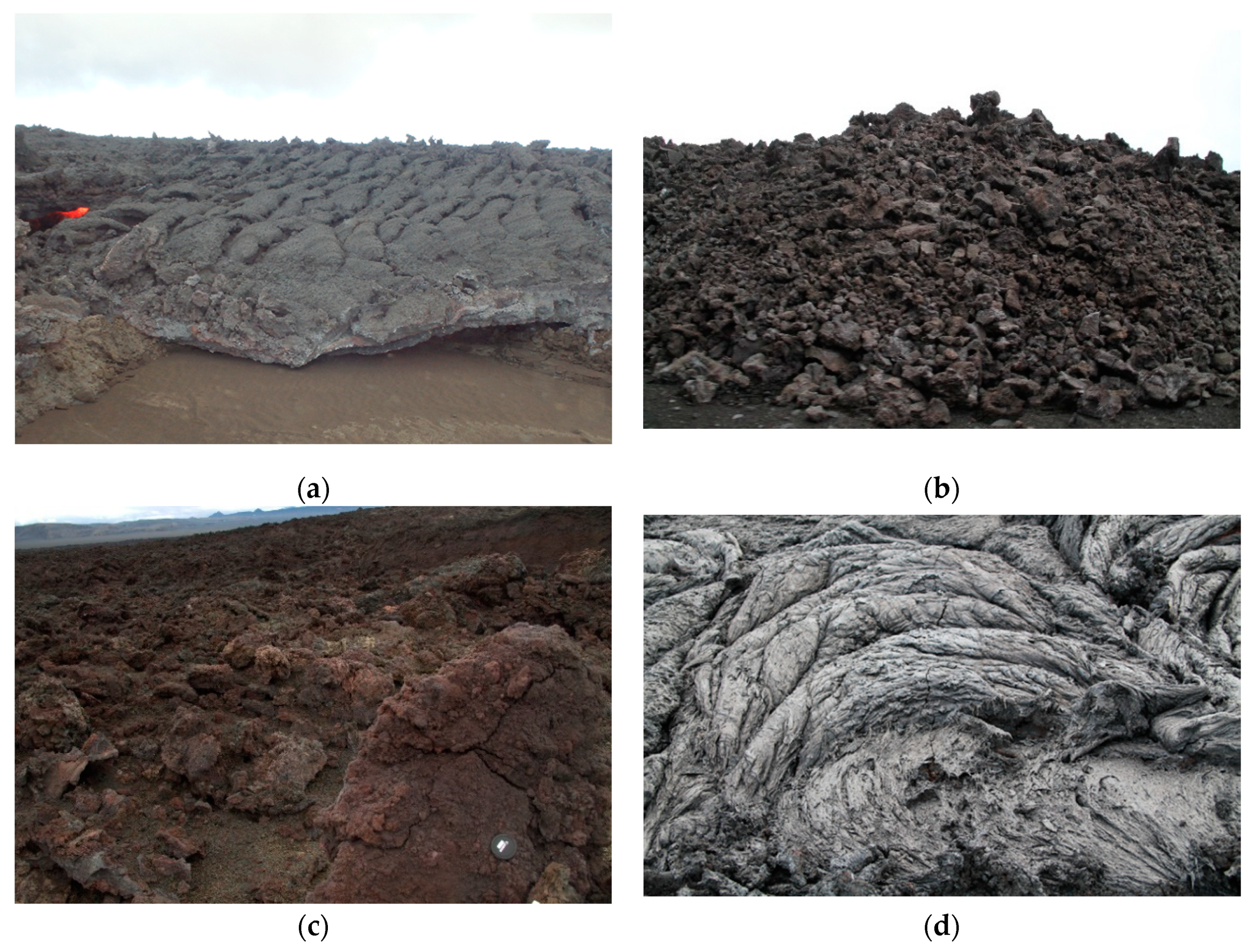
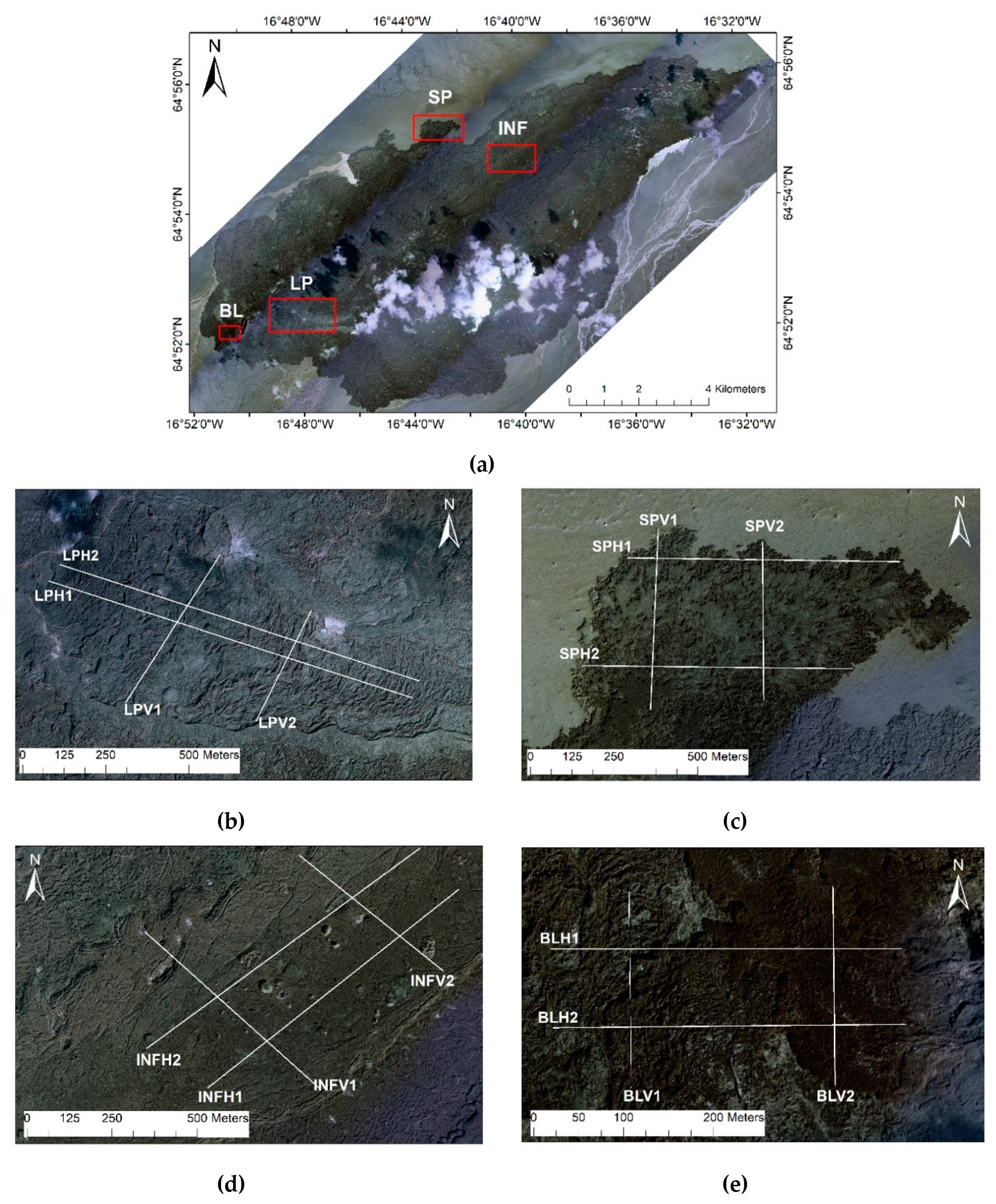
3. Morphology of the 2014–2015 Lava Flow at Holuhraun

The six months long eruption at Holuhraun 2014–2015 was the largest effusive eruption in Iceland in 230 years with an estimated bulk lava volume of 1.44 km3 [37,38,39]. The eruption is split into three phases based on the lava flow-field evolution [37]. The first phase was dominated by open channels, and during the second phase, lava emplacement was affected by the formation of a 1 km2 lava pond about 1 km downstream of the vent [37]. This pond became the main distribution point for the lava during this phase, controlling the emplacement of lava flows. Near the end of the second phase, vertical stacking of lava lobes became more prevalent, and lava tubes developed within the channel system, resulting in the formation of inflation plateaus [37]. In the final phase, transport of lava through tubes continued, and inflation plateaus grew in extent, raising the original channel surface by 5–10 m above the surrounding lava. Over 19 km2 of the flow field was resurfaced via surface breakouts from the closed paths during this period. Pedersen et al. [37] suggest that the topography of the lava field and surrounding made it possible to build an open channel system that was at minimum 5–10 m higher than the fluid lava. This system increased the static lava pressure, which was enough to lift the roof of the lava channels creating the inflation plateaus, allowing new lava to be transported to the distal ends of the lava field.
During the three phases of the 2014–2015 eruption, major changes in surface morphology of the lava occurred several times [37,40]. According to Pedersen et al. [37], shelly pahoehoe, slabby pahoehoe, rubbly pahoehoe, spiny pahoehoe, and aa were observed within the first week of the eruption. During the first phase and the second phase, aa was the dominant flow morphology of lava flows, and in the final phase, spiny pahoehoe was the main lava morphology [37]. This change from aa and pahoehoe morphology in the first and second phases to spiny pahoehoe in the final phase makes Holuhraun a paired lava flow-field. A paired lava flow-field is formed due to the decline of the effusion rate over the course of an eruption [41]. The Holuhraun lava flow-field was emplaced on a low-slope floodplain, and the chemical composition of the lava was uniform throughout the whole eruption [42,43]. This suggests that neither the topography nor the lava composition was the main factor for the observed changes in flow morphology [37]. The first transition of slabby pahoehoe to rubbly pahoehoe to aa occurred downstream of the vent, which is consistent with such changes in other lava producing eruptions and is explained by increased viscosity due to mixing, cooling, and gas loss during lava transport [34,37].
In this study, we examined roughness over lava flow surfaces in four locations depicted in Figure 2 that exhibit the known lava flow morphology at Holuhraun [7,37,44]. These lava flow features are: (1) lava pond, (2) spiny pahoehoe, (3) inflated channel, and (4) blocky surface. The lava pond formed during the first phase of the eruption [37]. Ropy folds preserved on the surface of a lava pond (Figure 1d) indicate slowly moving, low viscosity pahoehoe flows, which develop in response to the shortening of the flow surface in basaltic eruptions [30]. At the Holuhraun lava flow-field, spiny lava is characterized by a network of interconnected lobes that form inflated sheet-like flow units with rough spinose surfaces [7]. The millimeter-scale spines on the surface of these flows resemble the texture of aa, but the flow surfaces are generally continuous and are not decomposed into clinker [7]. Spiny lava units are the dominant flow type along most of the flow margins, except near the NE margin of the flow [7]. The inflated channel formed towards the end of the second phase to the final phase [37]. This surface feature maintains the morphology of the flow channel but increases in thickness. Pahoehoe flows are typically identified as inflated lava flows, but aa type flows may also inflate under certain circumstances [45]. In this study, we use the term blocky surface to avoid confusion with rubbly lava. Blocky surface is composed of larger blocks than rubbly. Similar to rubbly lava this feature likely formed due to continued auto-brecciation of crustal slabs into blocks of material through mechanical collisions between the slabs during transport [26].At Holuhraun lava flow-field, blocky surfaces are mostly found close to the vent. These lava flows were analyzed using the approach described in Section 4, and the results for the roughness analysis are presented in Section 5.

4. Datasets and Methods

To assess the surface roughness of lava flow features, we use high-DEM from two different sources. We focus on a subset of these data, obtained at four different facies on the lava flow-field. The datasets used in this study are described further in Table 2 and Section 4.1

4.1. Airborne LiDAR and Photogrammetry

Airborne LiDAR data, collected and processed by the Natural Environment Research Council (NERC) was acquired on September 4, 2015. We processed the point clouds to obtain 1 m spatial resolution over the lava flow-field with a vertical resolution of 4–5 cm (depending on the flight line). This was done using ENVI LiDAR 5.3 software. Eight flight lines were flown over Holuhraun: seven of these are parallel and aligned with the long axis of the field, while the eighth is transverse and crosses all the others (Figure 3a). The LiDAR measurements, therefore, do not cover the entirety of the flow-field. Furthermore, small clouds and fumaroles obscured parts of the lava and created gaps in the data. We sought to determine the surface roughness of the 2014–2015 lava flows at Holuhraun. DEMs are produced upon processing of point-clouds for a variety of lava flow textures around the study area.
We used photogrammetry-derived DEM provided by Loftmyndir ehf using data taken on August 30, 2015. Clouds obscured in some parts of the 2014–2015 Holuhraun lava flow-field (Figure 2). This Photogrammetry-derived DEM has a spatial resolution of 5 m (Figure 3b).

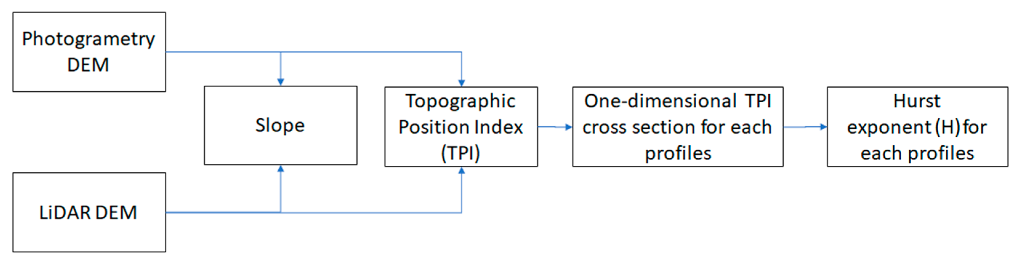
4.2. Deriving Surface Roughness
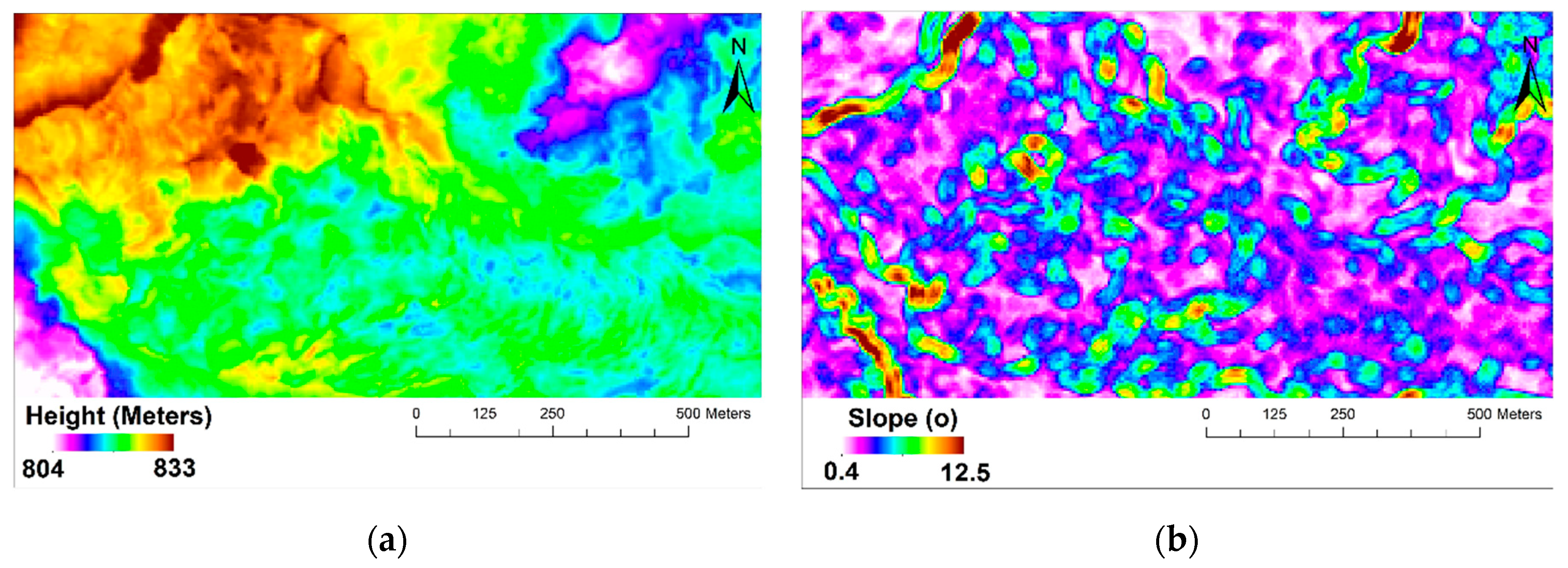
The methodology adopted for the assessment of the roughness is given in a sequential manner in Figure 4. In this study, we use TPI and one-dimensional H to quantify roughness values in the 2014–2015 Holuhraun lava flows from both photogrammetry DEM and LiDAR DEM. Finally, we determined the roughness properties for four different facies on the lava flow-field from Figure 2.

4.2.1. Slope

The estimation of slope from a regularly gridded DEM is a common procedure in terrain analysis [46,47]. The slope can be defined as a function of the gradients in the x and y direction at every point in a DEM:
s l o p e = arctan f x 2 + f y 2 .
The key in the slope estimation is the computation of the perpendicular gradients f x   and f y . We used moving 3 × 3 windows to derive local polynomial surface fit for the calculation [46,47]. This process was done using ArcGIS 10.6.

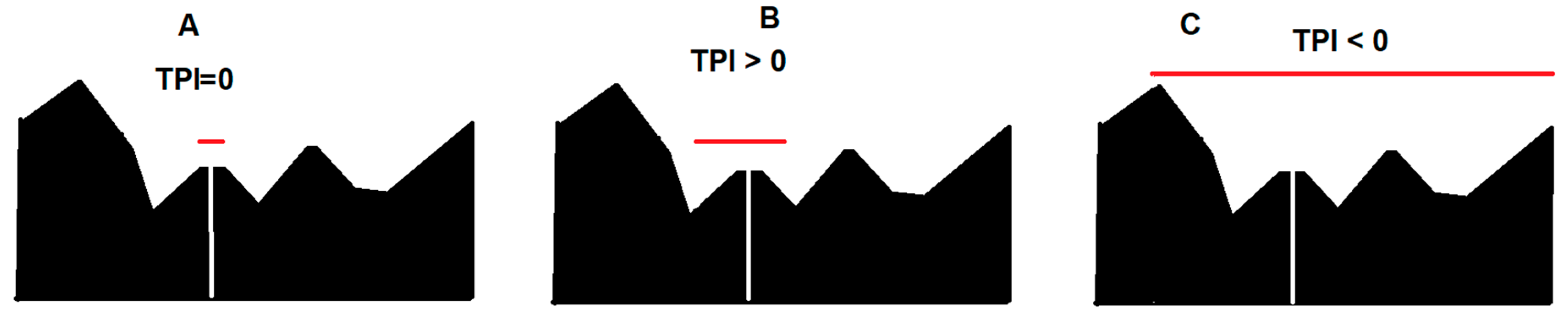
4.2.2. Topographic Position Index

In this study, topographic position index (TPI) [48] was used for deriving the roughness pattern of the lava flow-field. This method was originally created for use in ecology, geomorphology, and hydrology study [19,48] but has been recently used for assessing the topographic characteristics of lava flows [11]. TPI compares the elevation of each cell in a DEM to the mean elevation of a specified neighborhood around that cell. Mean elevation is subtracted from the elevation value at the center
T P I = C 0 C ¯ σ ,
where C 0 is the elevation of the model point under evaluation, C ¯ is the mean elevation of a gridpoint in the neighborhood, σ is the standard deviation of elevation in the neighborhood. Positive TPI indicates that a cell is higher in elevation (or more steeply sloping) than the average of its neighbors up to a specified distance away, whereas a negative one indicates that a cell is lower than the average of surrounding elevations (Figure 5) [19]. The cell neighborhood can be adapted to produce varying TPI values for different scales, thus changing the scale of roughness could affect the results [11,19,48]. In this study, we use a rectangular TPI with a 3 × 3 neighborhood size for both LiDAR DEM and photogrammetry DEM.

4.2.3. Hurst Exponent

In this study, we acquired a one-dimensional TPI profile over various lava flow surfaces in four locations in Figure 2. The profiles were typically a few hundred meters to kilometers long. Roughness properties may have directional biases [2,7,8]. In this study, profiles were collected in perpendicular directions (Figure 2). The Hurst exponent (H) is derived using rescaled range analysis (R/S) [15,49] for the TPI profiles. Equation (3) below shows the relation between R/S and H as
H = log ( R S ) log ( τ ) ,
where R is the difference between the maximum and minimum TPI detected in profiles, S is the standard deviation, and τ is the transect profiles. Hurst coefficient ranges from 0 to 1, where a higher H means a smooth or equally rough surface [2]. The mean Hurst exponent ( H ¯ ) was calculated for each lava unit.

5. Results

We extracted the slope, TPI, and Hurst exponent from the lava flow features in Figure 2 (lava pond, spiny pahoehoe, inflated channel, and blocky surface). Each lava feature displays TPI and H variations, although the entire range of H variation is not displayed at any individual flow. The roughness analysis results are shown as maps and profiles for each lava flow features. Based on the analysis, the surface feature that corresponds to a higher H and intermediate TPI pattern reflects a smoother surface than the lower H and irregular TPI patterns.

5.1. Lava Pond Roughness

For the photogrammetry DEM (Figure 6a), TPI and slope values at the lava pond ranged from −2.8 m to 2.8 m and from 0.4° to 12.5° (Figure 6b,c), respectively. For the LiDAR DEM (Figure 6d), TPI and slope values ranged from –3.2 m to 5.4 m and from 0.5° to 30° (Figure 6e,f), respectively. Both the LiDAR and photogrammetry derived TPI images have wave-like transitions patterns (Figure 6c,f). These patterns are also apparent from the slope (Figure 6b,e), indicating a relatively rough surface due to the ropy fold on the lava pond. Folds form where the velocity and viscosity of the lava surface decreases rapidly with depth [30]. This causes surface folding and irregular waviness in the surface which preserve on wave-like pattern on TPI maps.

5.2. Spiny Lava Roughness

The photogrammetry DEM (Figure 7a) had TPI and slope values at the spiny lava ranging from –1.8 m to 2.2 m and from 0° to 38° (Figure 7b,c), respectively. On the other hand, the LiDAR DEM (Figure 7d), had TPI and slope values ranging from –2.1 m to 1.8 m and from 0° to 36° (Figure 6e,f). The LiDAR DEM does not cover the entirety of the spiny lava due to gaps in the image. The low TPI values correspond to a low slope and indicate a flat and smooth surface that has formed from inflated spiny lava; however, we cannot differentiate the spinose pattern in this meter scale. The irregular transitions from low to high TPI and slope pattern around the flow margin might indicate a rough surface resulting from a breakout from the inflated spiny lava. These features will be explained in more detail in Section 6.2.

5.3. Inflated Channel Roughness

The photogrammetry DEM at the inflated channel (Figure 8a) yielded TPI and slope ranging from –3 m to 3.2 m and from 0.1° to 25° (Figure 8b,c), respectively. The LiDAR DEM (Figure 8d) yielded TPI and slope values ranging from –11 m to 4.8 m and from 0° to 33° (Figure 8e,f). Comparable to what we have found in spiny lava, low TPI patterns that correspond to a low slope were assigned to the flat surface of the inflated channel. The lowest TPI values correspond to a high slope indicating inflation pits and cracks. Inflation pits form where a portion of the flow is not inflating. The highest TPI values correspond to a high slope relating to boulders and grooves within the lava. The irregular transitions pattern from a low to a high slope and TPI values around the inflation margin are similar to what we have found on spiny lava. This indicates this feature is a rough surface that results from a breakout from the inflated channel (see Section 6.2 for more detail).

5.4. Block Surface Roughness

The photogrammetry DEM (Figure 9a) at the blocky surface units had TPI and slope ranging from –2.1 m to 2 m and from 0.4° to 15°, respectively (Figure 9a,b). The LiDAR DEM (Figure 9d) had TPI, and slope values ranging from −2.3 m to 2.3 m and from 0° to 23°, respectively (Figure 9e,f). In the LiDAR, blocky surface, typically, had irregular TPI patterns. These patterns indicate that the surface is rough which related to the decimeter to meter scale blocks of fragmented pahoehoe-like crust. However, in the photogrammetry DEM, blocky surface appears to have smoother patterns corresponding to high slope since the roughness of the blocky surface is not distinct in lower resolution.

5.5. Hurst Exponent Derived Roughness

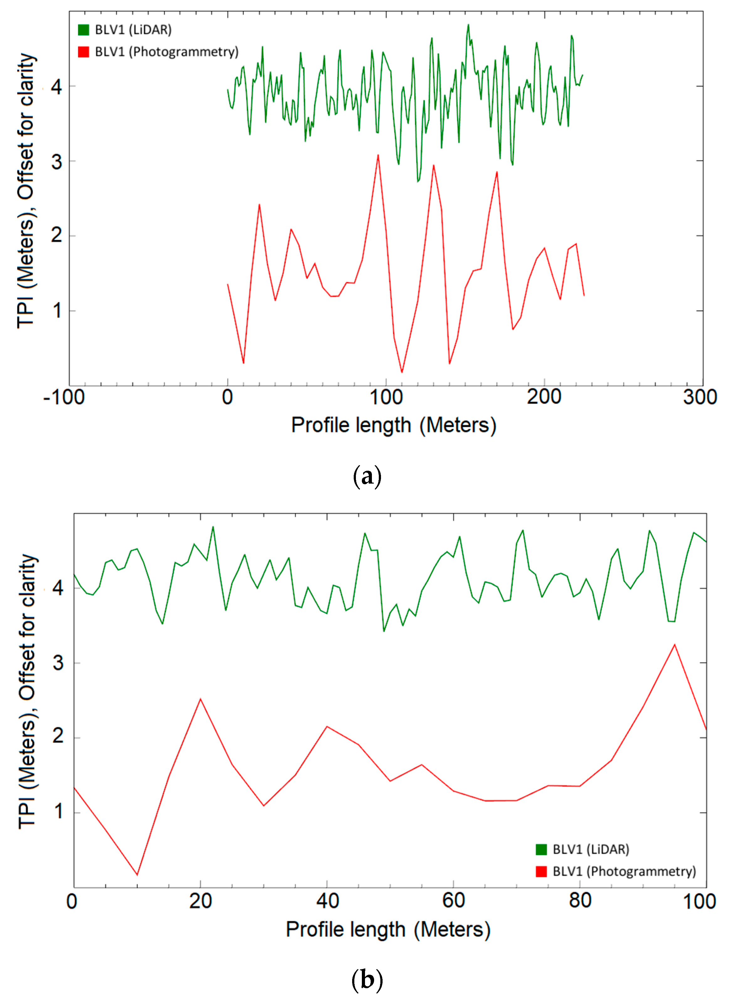
One Dimensional TPI Profiles

The one-dimensional TPI profiles over the four lava flow units are shown in Figure 10a–d. Based on H reported in Table 3, the surface roughness of lava features falls within the range from 0.3 ± 0.05 to 0.76 ± 0.04. Typically, LiDAR DEM yields lower Hurst exponent values than photogrammetry DEM. This was also found for blocky surface, i.e., photogrammetry DEM had higher Hurst exponent than LiDAR DEM. LiDAR DEM has greater pixel resolution than photogrammetry DEM which results in more detailed TPI profiles. This issue will be addressed in Section 6.1. Based on the Mean Hurst exponent ( H ¯ ), the roughest surface is the blocky surface with H ¯ ’ around 0.52 ± 0.04 and the inflated lava field appears to be the smoothest surface of these four lava units with H ¯ around 0.61 ± 0.06. These results are comparable with the results from the TPI map pattern that showed that inflated lava appears to be the smoothest surface, and blocky is the roughest surface. In general, the Hurst exponent values have a strong tendency to be close to 0.5. This was also suggested by an early study by Shepard et al. [2] for geological surface roughness.

6. Discussion

In this work, we examined lava flows roughness in the 2014–2015 lava field at Holuhraun using TPI and one-dimensional H profiles. Both TPI and H successfully derived lava roughness on selected lava units at Holuhraun. However, there are still some issues. How does the scale affect the roughness results for both TPI and Hurst exponent? Is the ‘smooth’ surface still smooth for a different scale? How do we connect the roughness to the emplacement style? What can we improve to get a better roughness assessment? In this section, we address several issues related to (1) TPI neighborhood size and profile length, (2) Eruption condition and link roughness pattern with the emplacement style, and (3) alternative datasets and methods for deriving roughness.

6.1. TPI Neighborhood Size and Profile Length

TPI is naturally very scale dependent [11,19,48,50]. We should consider what scale is the most relevant for the study being analyzed [19]. The patterns produced by TPI vary on the scale that we use to analyze. Figure 11 shows an illustration of similar topography using different neighborhood sizes in TPI [19,51]. We test different TPI neighborhood sizes on LiDAR DEM spiny lava, as shown in Figure 12a–d. The 1 × 1 neighborhood size (Figure 12a) was not as clear as the larger scales to differentiate flow margins but appears to emphasize small features on the lava flows, which does not show in larger neighborhoods. James [11] recommends building a catalog of features presented at each scale. This could be useful in assessing the topographic characteristics of a lava flow surface.
We consider that there are at least two factors that affect the H values: (1) pixel size and (2) the profile length. Figure 13a shows TPI profiles representing blocky surface vertical profile (BLV1) from LiDAR DEM and photogrammetry DEM. The LiDAR DEM profile is rougher than the photogrammetry DEM since the spatial spacing (pixel size) in the LiDAR DEM is denser than photogrammetry DEM because the resolution is higher (1 m vs. 5 m). This spatial spacing issue corresponds to the TPI neighborhood size in Figure 11, where LiDAR DEM captures more detailed TPI value than photogrammetry DEM which affects the Hurst exponent derived roughness. Second, we also consider the profile length as a factor that affects the Hurst exponent values. In Figure 13b, we subset the first 100 m BLV1 profiles, and the Hurst exponent values for these subset profiles were increased for both topographies. For LiDAR DEM the Hurst exponent values are 0.55 ± 0.05 compared to 0.30 ± 0.05 for full profiles, and for photogrammetry DEM the Hurst exponent values are 0.48 ± 0.01 compared to 0.40 ± 0.05 for full profiles. These results not necessarily conclude that the shorter profiles will increase the Hurst exponent. Extended profiles also can increase the Hurst exponent since the profiles could be equally rough, which can represent a ‘smooth’ surface [2]. In many cases, it depends on the morphology that we are studying [2,3], and we should know the morphology. The other thing we found is that the direction of profiles could bias the Hurst exponent [7,52]. We recommend in a future study to build series of profiles that are rotated by some number of degrees to capture a wider range of directions around the surface area of interest to derive precise roughness. Some studies are currently developing three-dimensional roughness estimates based on a 3D Gaussian filter applied to DEM [53].

6.2. Eruption Condition and Link Quantitative Roughness with the Emplacement Style

Quantitative roughness measurement of lava flow features provides insight into the relative emplacement styles. In particular, higher H and intermediate TPI patterns suggest a smoother surface, which reflects relatively lower viscosity lavas than for the lower H and irregular TPI pattern. However, roughness variations do not directly distinguish between lava viscosity. To quantify precise viscosity, more factors need to consider rather than single roughness. The difference in viscosity may be the result of transport within an insulated distributary system that limits heat loss. If the differences between the flow types are predominantly textural, local supply may be a controlling factor [5].
The two primary roughness identified in the, a smooth surface possibly inflated flow type and a rough surface possibly breakout, blocky surface and ropy fold data. Section 5.2 and Section 5.3 shows that smoother surface types exhibit morphologic properties attributed to flow inflation. Along margins, irregular transitions TPI pattern supports the interpretation of the occurrence of breakout (Figure 7c–f and Figure 8c–f). As displayed clearly in Figure 14a–b, the rough surface in lava flow margins from the three-dimension LiDAR surface model. These rough surfaces result from a breakout from the inflated surface from both spiny lava (Figure 14a) and inflated channel (Figure 14b). It is reported by Pedersen et al. [37] that a series of breakouts occurred during the third phase of the eruption, mostly in the flow margin and also in inflated channels. This breakout is inferred from the false color on the Earth Observing 1 (EO-1) Advanced Land Imager (ALI) satellite during the eruption (Figure 15). These breakouts occurred around 16 January 2015, a breakout from spiny lava and inflated channel. A breakout is a lobe originating from the liquid interior of active lava. It may take place through a crack at the front or the side of the flow margin when lava is inflated [54]. Injection of fresh basaltic magma into an established flow produces new breakouts of lava and promotes lifting of the upper crust (inflation). These breakout phenomena illustrated in Figure 16.

6.3. Alternative Datasets and Methods for Deriving Roughness

Recently, a number of and methods are used to quantify surface roughness. Neish et al. [7] quantified the surface roughness from synthetic aperture radar (SAR) using the circular polarization ratio (CPR). This technique is defined as the radar backscatter ratio in the same polarization that was transmitted (SC) to the opposite polarization (OC), where the CPR is SC divided by OC [7]. Rough surfaces tend to have approximately equal OC and SC returns, with CPR values approaching one. Meanwhile, the flat surfaces tend to have high OC returns and low CPR values [7]. We can also apply Hurst exponent to the radar backscattering profiles in order to derive roughness [15]. Neish et al. [7] also show that linking radar backscatter to the high-resolution topographic profiles is essential to understanding the structure of various geologic units. Another technique we could consider in describing roughness is optical images (multispectral–hyperspectral). Several studies characterize roughness from multispectral and hyperspectral based on the spectral reflectance [27,31,55,56]. The main assumption is that rough surface has lower reflectance than a smooth surface. The integration of these techniques with field measurement could improve surface roughness estimation of lava flow.

7. Conclusions

In this study, both TPI and one-dimensional H successfully derive quantitative flow roughness. The roughness assessment was acquired from four lava flow features: (1) spiny lava, (2) lava pond, (3) blocky surface, and (4) inflated channel. TPI patterns on spiny lava and inflated channels show that the intermediate TPI patterns with low slope indicate flat and smooth surface. Lava pond has transitions pattern from low to high TPI values forming a wave-like pattern. Meanwhile, irregular transitions from low to high TPI and the slope patterns indicate a rough surface that is found in blocky surface and flow margins, indicating lava breakouts. Quantitative measures of surface roughness of lava features fall within the H ranges from 0.30 ± 0.05 to 0.76 ± 0.04. The roughest surface is the blocky surface, and the inflated lava flow appears to be the smoothest surface among these four lava units. In general, the Hurst exponent values in the 2014–2015 lava field at Holuhraun has a strong tendency to be close to 0.5, which has good agreement with an earlier study for geological surface roughness. Neighborhood size is a critical component for TPI to quantify the roughness. Small neighborhoods capture small and local features and valleys, while large neighborhoods capture larger-scale features. We consider that there are at least two factors that affect the Hurst exponent values: (1) pixel size and (2) the profile length. We recommend in a future study to build a series of profiles that are rotated by some number of degrees to capture a wider range of directions, in order to derive precise roughness. The integration of multimodal remote sensing datasets and field measurement can improve the estimation of surface roughness of lava flow.

Author Contributions

Conceptualization, implementation, and preparation of the manuscript, M.A.; Supervision, Á.H., M.O.U., I.J., and T.T. All authors have read and agreed to the published version of the manuscript.

Funding

The first author was supported by the Indonesia Endowment Fund for Education (LPDP) Grant No. 20160222025516, European Network of Observatories and Research Infrastructures for Volcanology (EUROVOLC), and Vinir Vatnajökuls during his Ph.D. project. LiDAR airborne datasets provided by The European Facility for Airborne Research (EUFAR) and airborne photogrammetry provided by Loftmyndir ehf.

Acknowledgments

The authors would thank to Christoper Hamilton and anonymous reviewers for their thoughtful and constructive comments for the manuscript.

Conflicts of Interest

The authors declare no conflict of interest.

References

  1. Mills, G.; Fotopoulos, G. On the estimation of geological surface roughness from terrestrial laser scanner point clouds. Geosphere 2013, 9, 1410–1416. [Google Scholar] [CrossRef]
  2. Shepard, M.K.; Bulmer, M.H.; Gaddis, L.R.; Plaut, J.J.; Campbell, B.A.; Farr, T. The roughness of natural terrain: A planetary and remote sensing perspective. J. Geophys. Res. Space Phys. 2001, 106, 32777–32795. [Google Scholar] [CrossRef]
  3. Gaddis, L.R.; Mouginis-Mark, P.J.; Hayashi, J.N. Lava flow surface textures: SIR-B radar image texture, field observations, and terrain measurements. Photogramm. Eng. Remote Sens. 1990, 56, 211–224. [Google Scholar]
  4. Campbell, B.A.; Shepard, M.K. Lava flow surface roughness and depolarized radar scattering. J. Geophys. Res. Space Phys. 1996, 101, 18941–18951. [Google Scholar] [CrossRef]
  5. Crown, D.A.; Ramsey, M. Morphologic and thermophysical characteristics of lava flows southwest of Arsia Mons, Mars. J. Volcanol. Geotherm. Res. 2017, 342, 13–28. [Google Scholar] [CrossRef] [Green Version]
  6. Whelley, P.; Garry, W.B.; Hamilton, C.W.; Bleacher, J. LiDAR-derived surface roughness signatures of basaltic lava types at the Muliwai a Pele Lava Channel, Mauna Ulu, Hawai‘i. Bull. Volcanol. 2017, 79, 79. [Google Scholar] [CrossRef]
  7. Neish, C.; Hamilton, C.; Hughes, S.; Nawotniak, S.K.; Garry, W.; Skok, J.; Elphic, R.; Schaefer, E.; Carter, L.; Bandfield, J.; et al. Terrestrial analogues for lunar impact melt flows. Icarus 2017, 281, 73–89. [Google Scholar] [CrossRef]
  8. Morris, A.; Anderson, F.S.; Haldemann, A.F.C.; Brooks, B.A.; Foster, J.; Mouginis-Mark, P.J. Roughness of Hawaiian volcanic terrains. J. Geophys. Res. Space Phys. 2008, 113. [Google Scholar] [CrossRef]
  9. Anderson, S.W.; Stofan, E.; Plaut, J.J.; Crown, D.A. Block size distributions on silicic lava flow surfaces: Implications for emplacement conditions. GSA Bull. 1998, 110, 1258–1267. [Google Scholar] [CrossRef]
  10. Byrnes, J.M. Lava Flow Field Emplacement Studies on Mauna Ulu (Kilauea, Volcano, Hawai’i, USA) and Venus, Using Field and Remote Sensing Analyses. Ph.D. Thesis, University of Pittsburgh, Pittsburgh, PA, USA, 2002; pp. 1–212. [Google Scholar]
  11. James, D.H. Comparing Terrestrial and Extraterrestrial Lava Surface Roughness Using Digital Elevation Models From High Resolution Topography and Structure From Motion. Master’s Thesis, University of Northern Colorado, Greeley, CO, USA, 2019. [Google Scholar]
  12. Richardson, P.W.; Karlstrom, L. The multi-scale influence of topography on lava flow morphology. Bull. Volcanol. 2019, 81, 21. [Google Scholar] [CrossRef]
  13. Favalli, M.; Fornaciai, A.; Nannipieri, L.; Harris, A.; Calvari, S.; Lormand, C. UAV-based remote sensing surveys of lava flow fields: A case study from Etna’s 1974 channel-fed lava flows. Bull. Volcanol. 2018, 80, 29. [Google Scholar] [CrossRef]
  14. Gharechelou, S.; Tateishi, R.; Johnson, B.A. A Simple Method for the Parameterization of Surface Roughness from Microwave Remote Sensing. Remote. Sens. 2018, 10, 1711. [Google Scholar] [CrossRef] [Green Version]
  15. Aufaristama, M.; Höskuldsson, Á.; Jónsdóttir, I.; Ulfarsson, M.; Thordarson, T. New Insights for Detecting and Deriving Thermal Properties of Lava Flow Using Infrared Satellite during 2014–2015 Effusive Eruption at Holuhraun, Iceland. Remote. Sens. 2018, 10, 151. [Google Scholar] [CrossRef] [Green Version]
  16. Mallonee, H.C.; Kobs Nawotniak, S.E.; McGregor, M.; Hughes, S.S.; Neish, C.D.; Downs, M.; Delparte, D.; Lim, D.S.S.; Heldmann, J.L.; Team, F. Lava flow morphology classification based on measures of roughness. In Proceedings of the 48th Lunar and Planetary Science Conference, The Woodlands, TX, USA, 20–24 March 2017. [Google Scholar]
  17. Witt, T.; Walter, T.R.; Müller, D.; Guðmundsson, M.T.; Schöpa, A. The relationship between lava fountaining and vent morphology for the 2014–2015 Holuhraun eruption, Iceland, analyzed by video monitoring and topographic mapping. Front. Earth Sci. 2018, 6, 235. [Google Scholar] [CrossRef]
  18. Kereszturi, G.; Németh, K.; Moufti, M.R.; Cappello, A.; Murcia, H.; Ganci, G.; Del Negro, C.; Procter, J.; Zahran, H.M.A. Emplacement conditions of the 1256AD Al-Madinah lava flow field in Harrat Rahat, Kingdom of Saudi Arabia—Insights from surface morphology and lava flow simulations. J. Volcanol. Geotherm. Res. 2016, 309, 14–30. [Google Scholar] [CrossRef]
  19. Jennes, J. Topographic Position Index (tpi_jen.avx) Extension for ArcView 3.x, v. 1.3a; Jenness Enterprises: Flagstaff, AZ, USA, 2006; pp. 1–43. [Google Scholar]
  20. Swanson, D.A. Pahoehoe Flows from the 1969–1971 Mauna Ulu Eruption, Kilauea Volcano, Hawaii. GSA Bull. 1973, 84, 615. [Google Scholar] [CrossRef]
  21. Lopes, R.M.C.; Kilburn, C.R.J. Emplacement of lava flow fields: Application of terrestrial studies to Alba Patera, Mars. J. Geophys. Res. Space Phys. 1990, 95, 14383. [Google Scholar] [CrossRef]
  22. Diniega, S.; Smrekar, S.E.; Anderson, S.; Stofan, E.R. The influence of temperature-dependent viscosity on lava flow dynamics. J. Geophys. Res. Earth Surf. 2013, 118, 1516–1532. [Google Scholar] [CrossRef] [Green Version]
  23. Ramsey, M.S.; Fink, J.H. Estimating silicic lava vesicularity with thermal remote sensing: A new technique for volcanic mapping and monitoring. Bull. Volcanol. 1999, 61, 32–39. [Google Scholar] [CrossRef]
  24. Guest, J.E.; Duncan, A.M.; Stofan, E.R.; Anderson, S.W. Effect of slope on development of pahoehoe flow fields: Evidence from Mount Etna. J. Volcanol. Geotherm. Res. 2012, 219, 52–62. [Google Scholar] [CrossRef]
  25. Kilburn, C.R.J. Lava flows and flow fields. In Encyclopedia of Volcanoes; Sigurdsson, H., Ed.; Academic Press: San Diego, CA, USA, 2000; pp. 291–305. [Google Scholar]
  26. Hamilton, C.W. Fill and spill” lava flow emplacement: Implications for understanding planetary flood basalt eruptions. In NASA Technical Memorandum: Marshall Space Flight Center Faculty Fellowship Program; Six, N., Karr, G., Eds.; NASA Marshall Space Flight Center: Huntsville, AL, USA, 2019; pp. 47–56. [Google Scholar]
  27. Byrnes, J.M.; Ramsey, M.S.; Crown, D. A Surface unit characterization of the Mauna Ulu flow field, Kilauea Volcano, Hawai′i, using integrated field and remote sensing analyses. J. Volcanol. Geotherm. Res. 2004, 135, 169–193. [Google Scholar] [CrossRef]
  28. Griffiths, R.W.; Fink, J.H. The morphology of lava flows in planetary environments: Predictions from analog experiments. J. Geophys. Res. Space Phys. 1992, 97, 19739. [Google Scholar] [CrossRef]
  29. Anderson, S.W.; Fink, J.H. The Development and Distribution of Surface Textures at the Mount St. Helens Dome; Springer Science and Business Media LLC: Berlin/Heidelberg, Germany, 1990; Volume 2, pp. 25–46. [Google Scholar]
  30. Fink, J.H.; Fletcher, R.C. Ropy pahoehoe: Surface folding of a viscous fluid. J. Volcanol. Geotherm. Res. 1978, 4, 151–170. [Google Scholar] [CrossRef]
  31. Byrnes, J.M.; Crown, D.A. Morphology, stratigraphy, and surface roughness properties of Venusian lava flow fields. J. Geophys. Res. Space Phys. 2002, 107, 9-1. [Google Scholar] [CrossRef] [Green Version]
  32. Moore, R.B.; Clague, D.A.; Rubin, M.; Bohrson, W.A. Volcanism in Hawaii; U.S. Geological Survey Professional Paper 1350; U.S. Geological Survey: Reston, VA, USA, 1987. [Google Scholar]
  33. Wall, S.; Farr, T.; Muller, J.-P.; Lewis, P.; Leberl, F. Measurement of surface microtopography using helicopter-mounted stereo film cameras and two stereo matching techniques. In Proceedings of the 12th Canadian Symposium on Remote Sensing Geoscience and Remote Sensing Symposium, Vancouver, BC, Canada, 10–14 July 1989. [Google Scholar]
  34. Cashman, K.V.; Thornber, C.; Kauahikaua, J.P. Cooling and crystallization of lava in open channels, and the transition of Pāhoehoe Lava to ’A’ā. Bull. Volcanol. 1999, 61, 306–323. [Google Scholar] [CrossRef]
  35. Whelley, P.; Glaze, L.S.; Calder, E.S.; Harding, D.J. LiDAR-Derived Surface Roughness Texture Mapping: Application to Mount St. Helens Pumice Plain Deposit Analysis. IEEE Trans. Geosci. Remote. Sens. 2013, 52, 426–438. [Google Scholar] [CrossRef]
  36. Bretar, F.; Arab-Sedze, M.; Champion, J.; Pierrot-Deseilligny, M.; Heggy, E.; Jacquemoud, S. An advanced photogrammetric method to measure surface roughness: Application to volcanic terrains in the Piton de la Fournaise, Reunion Island. Remote. Sens. Environ. 2013, 135, 1–11. [Google Scholar] [CrossRef]
  37. Pedersen, G.B.M.; Höskuldsson, A.; Dürig, T.; Thordarson, T.; Jónsdóttir, I.; Riishuus, M.S.; Óskarsson, B.V.; Dumont, S.; Magnusson, E.; Gudmundsson, M.T.; et al. Lava field evolution and emplacement dynamics of the 2014–2015 basaltic fissure eruption at Holuhraun, Iceland. J. Volcanol. Geotherm. Res. 2017, 340, 155–169. [Google Scholar] [CrossRef] [Green Version]
  38. Bonny, E.; Thordarson, T.; Wright, R.; Höskuldsson, Á.; Jonsdottir, I. The Volume of Lava Erupted During the 2014 to 2015 Eruption at Holuhraun, Iceland: A Comparison Between Satellite- and Ground-Based Measurements. J. Geophys. Res. Solid Earth 2018, 123, 5412–5426. [Google Scholar] [CrossRef]
  39. Diego, C.; Ripepe, M.; Marco, L.; Cigolini, C. Modelling satellite-derived magma discharge to explain caldera collapse. Geology 2017, 45, 523–526. [Google Scholar]
  40. Pedersen, G.; Höskuldsson, A.; Riishuus, M.S.; Jónsdóttir, I.; Thórdarson, T.; Gudmundsson, M.T.; Durmont, S. Emplacement dynamics and lava field evolution of the flood basalt eruption at Holuhraun, Iceland: Observations from field and remote sensing data. In Proceedings of the EGU General Assembly, Vienna, Austria, 17–22 April 2016; Volume 18, p. 13961. [Google Scholar]
  41. Rowland, S.K.; Walker, G.P. Pahoehoe and aa in Hawaii: Volumetric flow rate controls the lava structure. Bull. Volcanol. 1990, 52, 615–628. [Google Scholar] [CrossRef]
  42. Gíslason, S.; Stefánsdóttir, G.; Pfeffer, M.A.; Barsotti, S.; Jóhannsson, T.; Galeczka, I.; Bali, E.; Sigmarsson, O.; Stefánsson, A.; Keller, N.S.; et al. Environmental pressure from the 2014–15 eruption of Bárðarbunga volcano, Iceland. Geochem. Perspect. Lett. 2015, 1, 84–93. [Google Scholar] [CrossRef] [Green Version]
  43. Gudmundsson, M.T.; Jónsdóttir, K.; Hooper, A.; Holohan, E.; Halldórsson, S.A.; Ófeigsson, B.G.; Cesca, S.; Vogfjörd, K.S.; Sigmundsson, F.; Högnadóttir, T.; et al. Gradual caldera collapse at Bárdarbunga volcano, Iceland, regulated by lateral magma outflow. Science 2016, 353, aaf8988. [Google Scholar] [CrossRef] [PubMed] [Green Version]
  44. Aufaristama, M.; Höskuldsson, Á.; Ulfarsson, M.; Jónsdóttir, I.; Thordarson, T. The 2014–2015 Lava Flow Field at Holuhraun, Iceland: Using Airborne Hyperspectral Remote Sensing for Discriminating the Lava Surface. Remote. Sens. 2019, 11, 476. [Google Scholar] [CrossRef] [Green Version]
  45. Hargitai, H. Inflated lava flow. In Encyclopedia of Planetary Landforms; Hargitai, H., Kereszturi, Á., Eds.; Springer: New York, NY, USA, 2015; pp. 1029–1034. [Google Scholar]
  46. Florinsky, I. Accuracy of local topographic variables derived from digital elevation models. Int. J. Geogr. Inf. Sci. 1998, 12, 47–62. [Google Scholar] [CrossRef]
  47. Zhou, Q.; Liu, X. Analysis of errors of derived slope and aspect related to DEM data properties. Comput. Geosci. 2004, 30, 369–378. [Google Scholar] [CrossRef]
  48. Guisan, A.; Weiss, S.B. GLM versus CCA spatial modeling of plant species distribution. Plant Ecol. 1999, 143, 107–122. [Google Scholar] [CrossRef]
  49. Liu, B.; Yao, L.; Fu, X.; He, B.; Bai, L. Application of the Fractal Method to the Characterization of Organic Heterogeneities in Shales and Exploration Evaluation of Shale Oil. J. Mar. Sci. Eng. 2019, 7, 88. [Google Scholar] [CrossRef] [Green Version]
  50. Hirzel, A.; Guisan, A. Which is the optimal sampling strategy for habitat suitability modelling. Ecol. Model. 2002, 157, 331–341. [Google Scholar] [CrossRef]
  51. Mokarram, M.; Roshan, G.; Negahban, S. Landform classification using topography position index (case study: Salt dome of Korsia-Darab plain, Iran). Model. Earth Syst. Environ. 2015, 1, 1–7. [Google Scholar] [CrossRef] [Green Version]
  52. Hamilton, C.W.; Mouginis-Mark, P.J.; Sori, M.M.; Scheidt, S.P.; Bramson, A.M. Episodes of Aqueous Flooding and Effusive Volcanism Associated With Hrad Vallis, Mars. J. Geophys. Res. Planets 2018, 123, 1484–1510. [Google Scholar] [CrossRef] [Green Version]
  53. Fan, K.; Neish, C.D.; Zanetti, M.; Kukko, A. An improved methodology for 3-dimensional characterization of surface roughness as applied to lava flows. In Proceedings of the 49th Lunar and Planetary Science Conference 2018, The Woodlands, TX, USA, 19–23 March 2018. [Google Scholar]
  54. Thordarson, T.; Self, S. The Roza Member, Columbia River Basalt Group: A gigantic pahoehoe lava flow field formed by endogenous processes? J. Geophys. Res. Space Phys. 1998, 103, 27411–27445. [Google Scholar] [CrossRef] [Green Version]
  55. Spinetti, C.; Mazzarini, F.; Casacchia, R.; Colini, L.; Neri, M.; Behncke, B.; Salvatori, R.; Buongiorno, M.F.; Pareschi, M.T. Spectral properties of volcanic materials from hyperspectral field and satellite data compared with LiDAR data at Mt. Etna. Int. J. Appl. Earth Obs. Geoinf. 2009, 11, 142–155. [Google Scholar] [CrossRef]
  56. Aufaristama, M.; Höskuldsson, Á.; Jonsdottir, I.; Ólafsdóttir, R. Mapping and Assessing Surface Morphology of Holocene Lava Field in Krafla (NE Iceland) Using Hyperspectral Remote Sensing. IOP Conf. Ser. Earth Environ. Sci. 2016, 29, 12002. [Google Scholar] [CrossRef] [Green Version]
Figure 1. Surface morphology on the 2014–2015 lava flow at Holuhraun. (a) Spiny pahoehoe flow on Holuhraun lava flow with a smooth, coherent crust at the meter scale (Photo was taken by Thorvaldur Thordarson). (b) Aa lava flow with brecciated flow tops and bases (Photo was taken by G.B.M. Pedersen). (c) A blocky surface that is composed of larger blocks than aa lava and these blocks have a larger surface area (Photo was taken by Muhammad Aufaristama). (d) Ropy folds observed in the channel flow and pond (Photo was taken by G.B.M. Pedersen).
Geosciences 10 00125 g001
Figure 2. An aerial photograph of the Holuhraun lava field (a) taken by Loftmyndir ehf with four different facies units (red boxes): (b) Lava pond (LP); (c) spinny pahoehoe (SP); (d) inflated channel (INF); and (e) blocky surface (BL). The white profiles are profiles used to derive the Hurst exponent. The horizontal and vertical profiles are collected for each unit marked with H1, H2, V1, and V2.
Geosciences 10 00125 g002
Figure 3. (a) The LiDAR DEM acquired on 4 September 2015, with a 1-meter pixel resolution. The LiDAR does not cover the entirety of the flow-field and has a gap in between the eight lines. (b) Photogrammetry-derived DEM based on an aerial photograph with a spatial resolution of 5 m.
Geosciences 10 00125 g003
Figure 4. The workflow processing to assess roughness from the lava flow from LiDAR and photogrammetry.
Geosciences 10 00125 g004
Figure 5. An illustration of the topographic position index (TPI) value in the topography, adapted, and modified from Jennes [19]. The red lines indicate the neighborhood size.
Geosciences 10 00125 g005
Figure 6. (a) DEM of lava pond derived from the photogrammetry image. (b) Slope of the lava pond derived from the photogrammetry DEM image. (c) TPI of lava pond derived from the photogrammetry DEM image. (d) DEM of lava pond derived from the LiDAR image. (e) TPI of lava pond derived from the DEM LiDAR image. (f) TPI lava pond derived from the DEM LiDAR image.
Geosciences 10 00125 g006aGeosciences 10 00125 g006b
Figure 7. (a) DEM of spiny lava derived from the photogrammetry image. (b) Slope of the spiny lava from derived from the photogrammetry DEM image. (c) TPI of spiny lava channel derived from the photogrammetry DEM. (d) DEM of spiny lava derived from the LiDAR. (e) TPI of spiny lava derived from the DEM LiDAR. (f) TPI of spiny lava derived from the DEM LiDAR.
Geosciences 10 00125 g007aGeosciences 10 00125 g007b
Figure 8. (a) DEM of the inflated channel derived from the photogrammetry image. (b) Slope of the inflated channel derived from the photogrammetry DEM. (c) TPI of the inflated channel derived from the photogrammetry DEM. (d) DEM of the inflated channel derived from the LiDAR. (e) TPI of the inflated channel derived from the DEM LiDAR. (f) TPI of the inflated channel derived from the DEM LiDAR.
Geosciences 10 00125 g008aGeosciences 10 00125 g008b
Figure 9. (a) DEM of blocky lava derived from the photogrammetry image. (b) The slope of the blocky surface derived from the photogrammetry DEM. (c) TPI of blocky surface derived from the photogrammetry DEM. (d) DEM of blocky lava derived from the LiDAR. (e) TPI of blocky surface derived from the DEM LiDAR. (f) TPI of blocky surface derived from the DEM LiDAR.
Geosciences 10 00125 g009aGeosciences 10 00125 g009b
Figure 10. TPI profiles representing four different lava units at the 2014–2015 Holuhraun lava flow in Iceland; (a) horizontal profiles derived from photogrammetry DEM; (b) horizontal profiles derived from LiDAR DEM; (c) vertical profiles derived from photogrammetry DEM; (d) vertical profiles derived from LiDAR DEM. The profiles had been offset from each other for clarity.
Geosciences 10 00125 g010
Figure 11. The illustration of the effects of the neighborhood size on TPI value adapted and modified from Jennes [19]. The red line depicts the neighborhood size. In topography (A), the neighborhood size is small enough that the point is at about the same elevation as the entire analysis region, so the TPI value is approximately 0, which means it is a flat surface. In topography (B), the neighborhood size is large enough to encompass the entire small hill, and the point is consequently much higher than its surroundings and has a correspondingly high TPI value resulting in that the point is detected as a ridge [19]. In topography (C), the neighborhood includes the hills on either side of the valley, and therefore the point is lower than its neighbors and has a negative TPI value [11,19].
Geosciences 10 00125 g011
Figure 12. TPI maps derived from LiDAR DEM at spiny lava for different neighborhood size (a) 1 × 1 neighborhood size; (b) 3 × 3 neighborhood size; (c) 5 × 5 neighborhood size; (d) 10 × 10 neighborhood size.
Geosciences 10 00125 g012
Figure 13. TPI profiles representing the first vertical profile of the blocky surface (BLV1) from the LiDAR DEM (green) and the photogrammetry DEM (red). (a) full profiles; (b) a zoom-in of the first 100 meters of (a). The profiles had been offset from each other for clarity.
Geosciences 10 00125 g013
Figure 14. Three-dimensional LiDAR surface model, white line indicating breakout and inflated surface. (a) Spiny lava flow margin. (b) Inflated channel flow margin.
Geosciences 10 00125 g014
Figure 15. (a) EO-ALI False color band 7,5,4′ on 16 January 2015 shows the high-temperature area during the eruption at Holuhraun. Boxes show series of breakout occurred in the flow margin, including on: (b) spiny lava and; (c) inflated channel margin.
Geosciences 10 00125 g015aGeosciences 10 00125 g015b
Figure 16. Cartoon illustrated the lava breakout. (a) A lava core exists within the lava channel/lobe under the visco-elastic crust. The lava core is contained within a visco-elastic skin covered by a brittle crust. (b) The lava flow became re-activated, and the lava core injected acted as a flow path promotes lifting of the upper crust (inflation). (c) Cracks formed on crust on the lava flow front/margin. (d) When the inflation continues, the crust eventually breaks, and breakouts leek from the margin or flow front of the inflated surface.
Geosciences 10 00125 g016
Table 1. Features Affecting Lava Flow Roughness at Different Scales, modified from James [11].
ScaleFlow FeaturesCommon MethodsResolutionReferences
Millimeter to centimeterGas bubble walls and minor folds/cracksMicroscope, Radar backscattering<1 cm[33,34]
Centimeter to meterFlow toes and blocksHurst exponent, RMS slope<1 m[2,7,11,33]
MeterTumuli, ridges, and crease patternsRadar backscatter, Hurst exponent~1 m[7,11,16,31]
More than decameterFull flow fields, flow marginRadar polarization>10 m[3,4,15]
Table 2. High-resolution DEM used in this study.
PlatformDate of AcquisitionAreaSpatial ResolutionSource
Airborne LiDAR4 September 2015100 km2
(Gap in between lines)
1 m
(processed in ENVI LiDAR 5.3)
NERC
Airborne photogrammetry30 August 2015167 km25 mLoftmyndir ehf
Table 3. Lava flow roughness properties at the 2014–2015 eruption at Holuhraun, derived from one-dimension TPI profiles for each lava unit.
ProfileLava FeatureLength (m)H (Photogrammetry)H (LiDAR) H ¯ (Mean)
LPH1Lava pond11500.53 ± 0.070.52 ± 0.050.55 ± 0.06
LPH2Lava pond11500.55 ± 0.060.43 ± 0.07
LPV1Lava pond5300.56 ± 0.060.6 ± 0.03
LPV2Lava pond3700.65 ± 0.050.57 ± 0.06
SPH1Spiny8100.52 ± 0.060.56 ± 0.050.58 ± 0.05
SPH2Spiny8100.65 ± 0.060.56 ± 0.05
SPV1Spiny5400.63 ± 0.04- *
SPV2Spiny4800.63 ± 0.040.54 ± 0.06
INFH1Inflated channel9500.66 ± 0.060.52 ± 0.040.61 ± 0.06
INFH2Inflated channel10000.69 ± 0.060.55 ± 0.06
INFV1Inflated channel6300.56 ± 0.070.56 ± 0.06
INFV2Inflated channel5400.76 ± 0.040.60 ± 0.05
BLH1Blocky surface3900.61 ± 0.040.49 ± 0.030.52 ± 0.04
BLH2Blocky surface3900.65 ± 0.050.56 ± 0.03
BLV1Blocky surface2200.4 ± 0.050.30 ± 0.04
BLV2Blocky surface2200.65 ± 0.050.52 ± 0.03
* was not acquired due to the gap in the LiDAR data.

