Controls on Gas Domains and Production Behaviour in A High-Rank CSG Reservoir: Insights from Molecular and Isotopic Chemistry of Co-Produced Waters and Gases from the Bowen Basin, Australia


 ,
,
Abstract
1. Introduction
2. Geological and Hydrogeological Setting
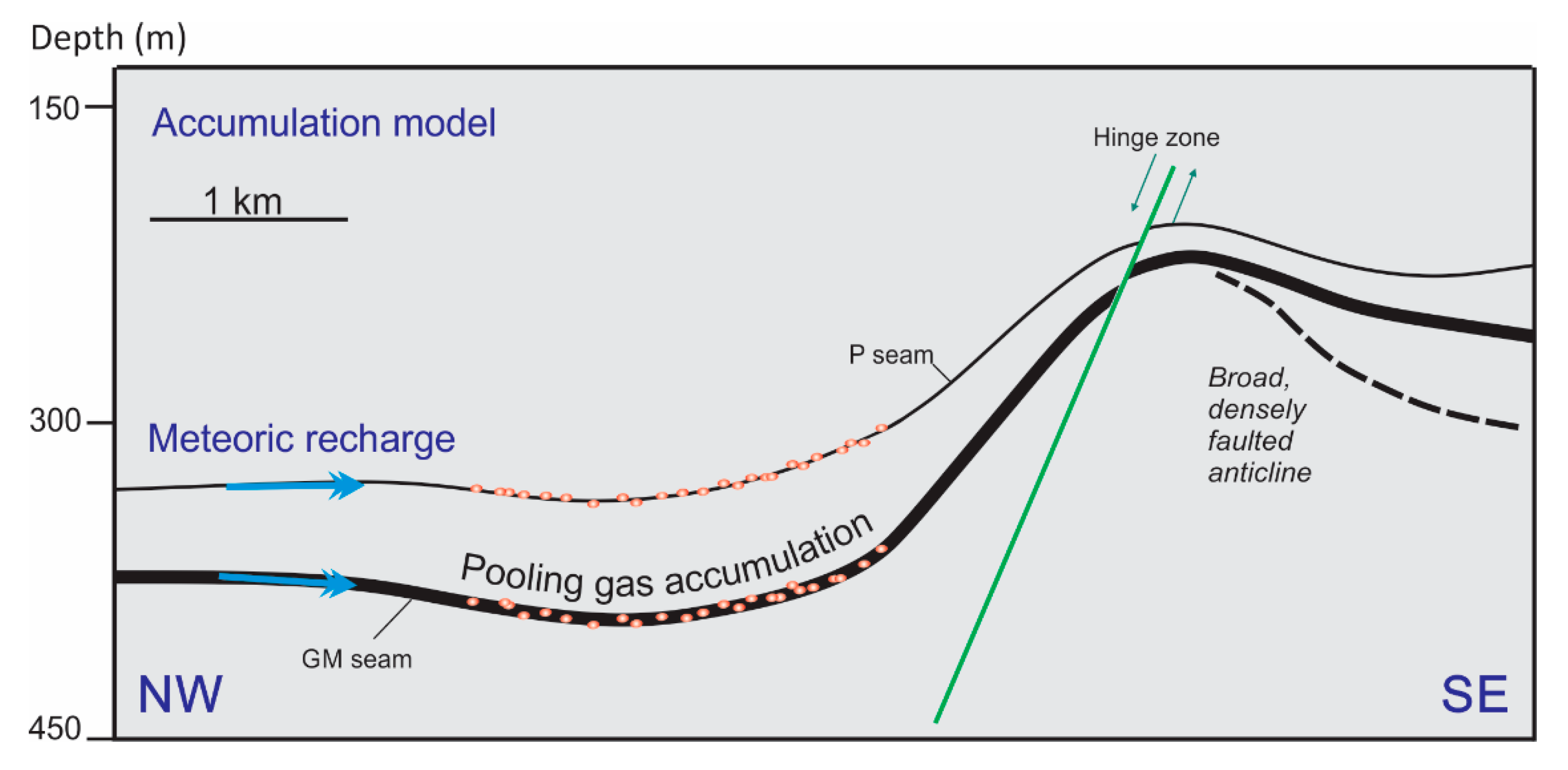
2.1. Gas Domains and Production Behaviour of the Study Field
Production Classes Assigned to Geochemical Study Samples
2.2. Previous Geochemical Investigations
2.3. This Study
3. Sampling and Methods
3.1. Standard Water Chemistry
3.2. Isotopic Analyses
3.2.1. Water Oxygen and Hydrogen Isotopes
3.2.2. Gas Hydrogen and Carbon Isotopes
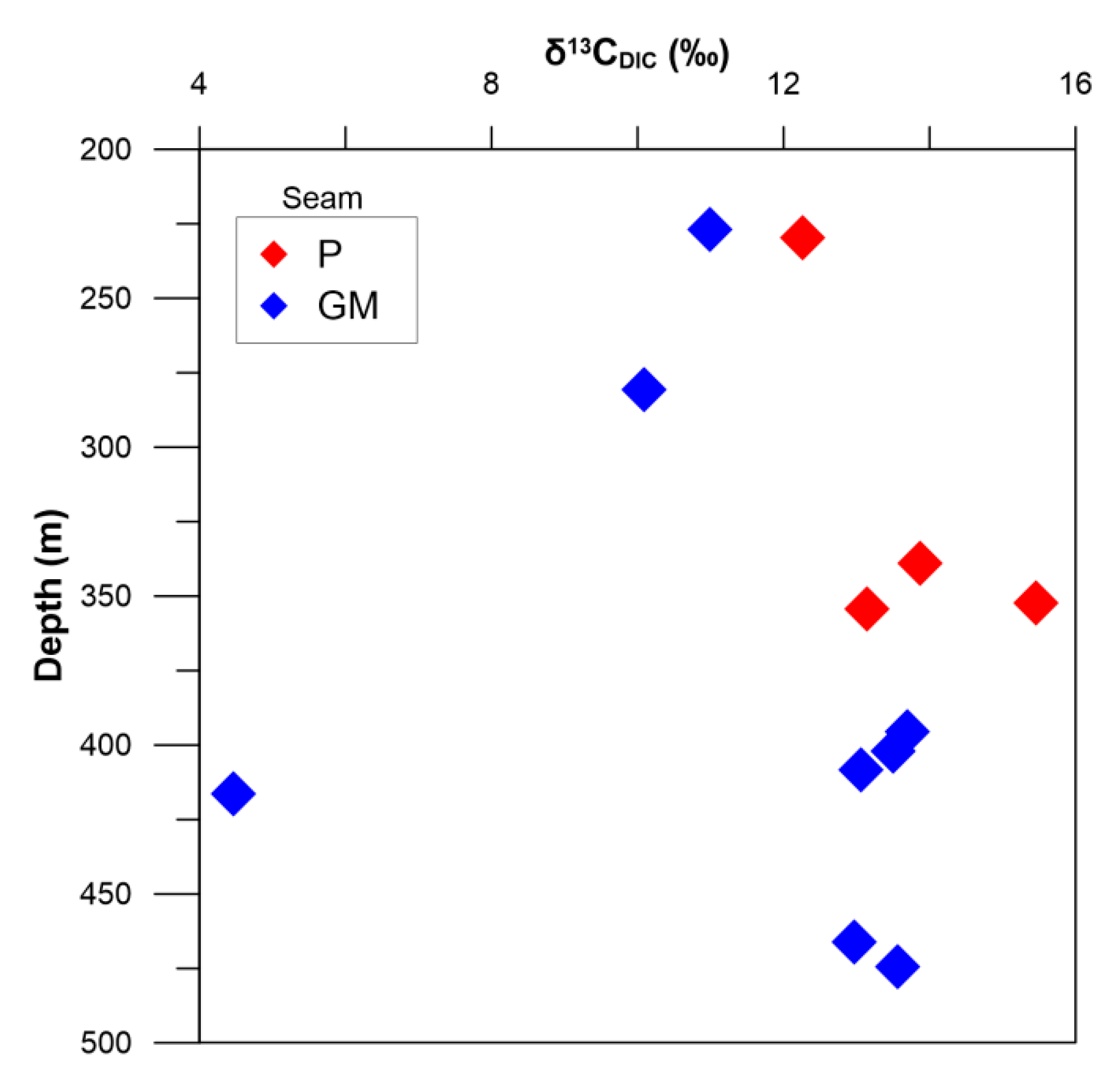
3.2.3. Dissolved Inorganic Carbon (δ13CDIC)
4. Results
4.1. Gas Isotopes
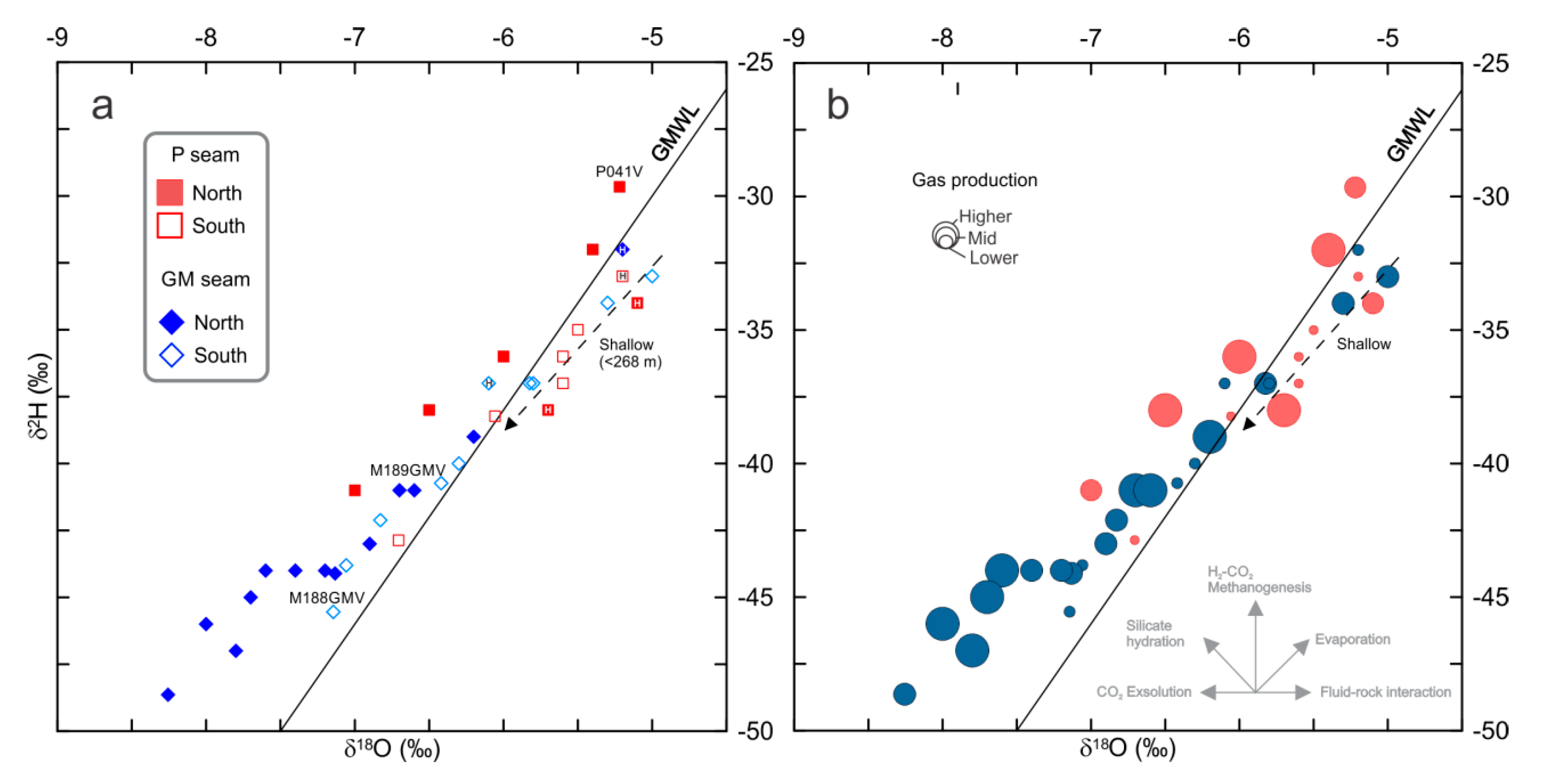
4.2. Water Isotopes
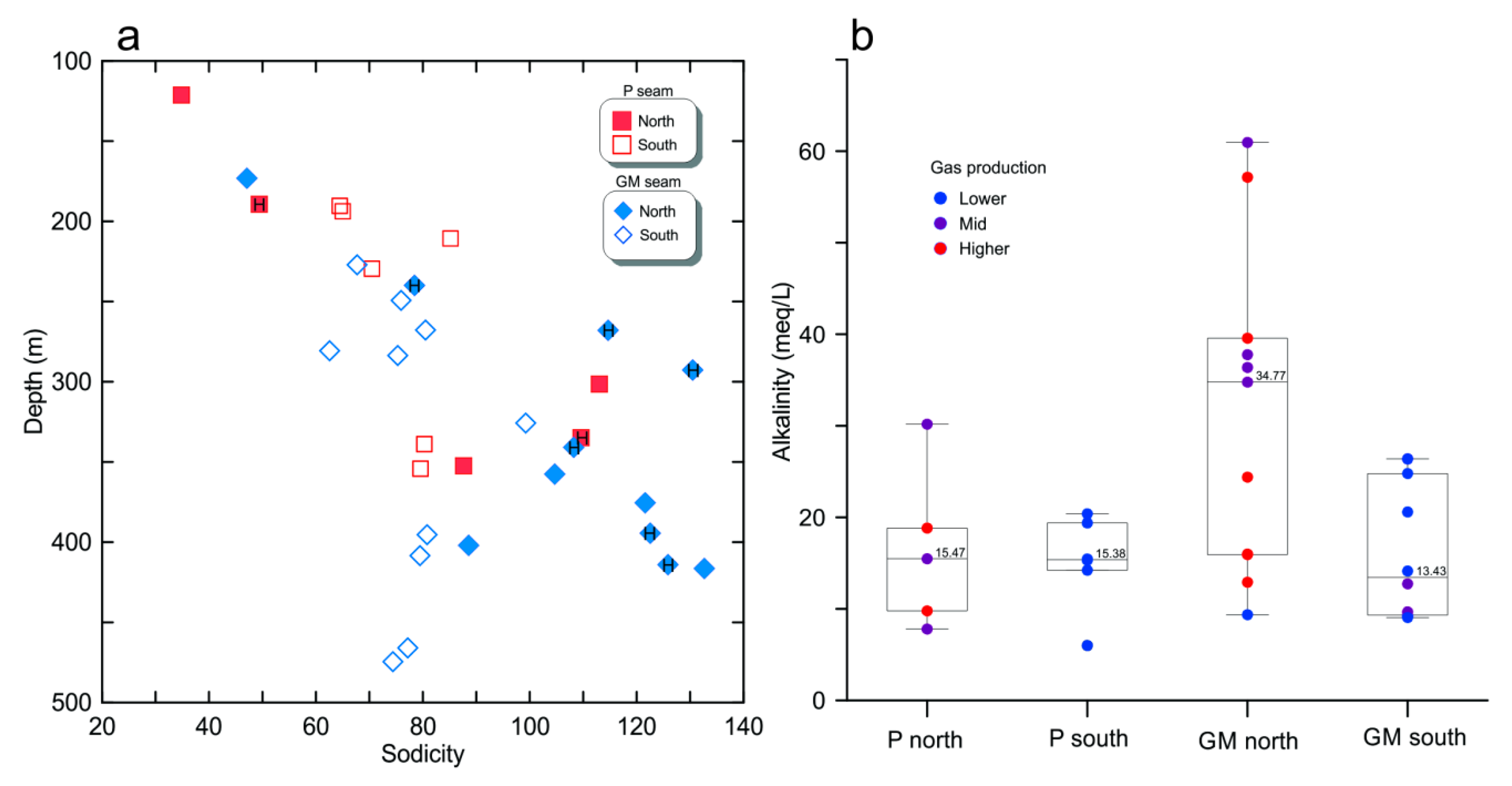
4.3. Water Chemistry
5. Discussion
5.1. Carbon Isotope System
5.1.1. Isotopic Evidence for Thermogenic Gas Charge
5.1.2. Isotopic Evidence for Extent of Methanogenesis
5.2. Hydrogen Isotope System
5.3. Hydrogeochemical Indicators of Microbial Methanogenesis
5.4. Value of Expanded Hydrochemical (Major Ions) and Stable Isotope Datasets for Understanding Gas Domains and Production Behaviour
6. Conclusions
Author Contributions
Funding
Acknowledgments
Conflicts of Interest
References
- Baublys, K.; Hamilton, S.; Golding, S.D.; Vink, S.; Esterle, J. Microbial controls on the origin and evolution of coal seam gases and production waters of the Walloon Subgroup; Surat Basin, Australia. Int. J. Coal Geol. 2015, 147, 85–104. [Google Scholar] [CrossRef]
- Golding, S.D.; Boreham, C.J.; Esterle, J.S. Stable isotope geochemistry of coal bed and shale gas and related production waters: A review. Int. J. Coal Geol. 2013, 120, 24–40. [Google Scholar] [CrossRef]
- Kinnon, E.; Golding, S.D.; Boreham, C.; Baublys, K.; Esterle, J. Stable isotope and water quality analysis of coal bed methane production waters and gases from the Bowen Basin, Australia. Int. J. Coal Geol. 2010, 82, 219–231. [Google Scholar] [CrossRef]
- McIntosh, J.C.; Warwick, P.D.; Martini, A.M.; Osborn, S.G. Coupled hydrology and biogeochemistry of Paleocene–Eocene coal beds, northern Gulf of Mexico. GSA Bull. 2010, 122, 1248–1264. [Google Scholar] [CrossRef]
- Scott, A.R.; Kaiser, W.; Ayers Jr, W.B. Thermogenic and Secondary Biogenic Gases, San Juan Basin, Colorado and New Mexico--Implications for Coalbed Gas Producibility. AAPG Bull. 1994, 78, 1186–1209. [Google Scholar]
- Strąpoć, D.; Mastalerz, M.; Dawson, K.; Macalady, J.; Callaghan, A.V.; Wawrik, B.; Turich, C.; Ashby, M. Biogeochemistry of Microbial Coal-Bed Methane. Annu. Rev. Earth Planet. Sci. 2011, 39, 617–656. [Google Scholar] [CrossRef]
- Van Voast, W.A. Geochemical signature of formation waters associated with coalbed methane. AAPG Bull. 2003, 87, 667–676. [Google Scholar] [CrossRef]
- Vinson, D.S.; Blair, N.E.; Martini, A.M.; Larter, S.; Orem, W.H.; McIntosh, J.C.; Larter, S. Microbial methane from in situ biodegradation of coal and shale: A review and reevaluation of hydrogen and carbon isotope signatures. Chem. Geol. 2017, 453, 128–145. [Google Scholar] [CrossRef]
- Burra, A.; Esterle, J.S.; Golding, S.D. Coal seam gas distribution and hydrodynamics of the Sydney Basin, NSW, Australia. Aust. J. Earth Sci. 2014, 61, 427–451. [Google Scholar] [CrossRef]
- Pashin, J.C. Hydrodynamics of coalbed methane reservoirs in the Black Warrior Basin: Key to understanding reservoir performance and environmental issues. Appl. Geochem. 2007, 22, 2257–2272. [Google Scholar] [CrossRef]
- Scott, A.R. Hydrogeologic factors affecting gas content distribution in coal beds. Int. J. Coal Geol. 2002, 50, 363–387. [Google Scholar] [CrossRef]
- Thomson, S.; Hatherly, P.; Hennings, S.; Sandford, J. A model for gas distribution in coals of the Lower Hunter, Sydney Basin. In Proceedings of the Eastern Australian Basins Symposium III, Sydney, Australia, 15–17 September 2008. [Google Scholar]
- Baublys, K.A.; Hamilton, S.K.; Hofmann, H.; Golding, S.D. A strontium (87Sr/86Sr) isotopic study on the chemical evolution and migration of groundwaters in a low-rank coal seam gas reservoir (Surat Basin, Australia). Appl. Geochem. 2019, 101, 1–18. [Google Scholar] [CrossRef]
- Draper, J.J.; Boreham, C. Geological controls on exploitable coal seam gas distribution in Queensland. APPEA J. 2006, 46, 343–366. [Google Scholar] [CrossRef]
- Faiz, M.; Hendry, P. Significance of microbial activity in Australian coal bed methane reservoirs—A review. Bull. Can. Pet. Geol. 2006, 54, 261–272. [Google Scholar] [CrossRef]
- Hamilton, S.; Golding, S.D.; Baublys, K.; Esterle, J. Stable isotopic and molecular composition of desorbed coal seam gases from the Walloon Subgroup, eastern Surat Basin, Australia. Int. J. Coal Geol. 2014, 122, 21–36. [Google Scholar] [CrossRef]
- Hamilton, S.; Golding, S.D.; Baublys, K.; Esterle, J. Conceptual exploration targeting for microbially enhanced coal bed methane (MECoM) in the Walloon Subgroup, eastern Surat Basin, Australia. Int. J. Coal Geol. 2015, 138, 68–82. [Google Scholar] [CrossRef]
- Smith, J.W.; Pallasser, R.J. Microbial Origin of Australian Coalbed Methane. AAPG Bull. 1996, 80, 891–897. [Google Scholar]
- Hillis, R.R.; Reynolds, S.D. In Situ Stress Field of Australia; Geological Society of Australia Special Publication: Hornsby, Australia, 2002; pp. 43–52. [Google Scholar]
- Beeston, J. Coal rank variation in the Bowen Basin, Queensland. Int. J. Coal Geol. 1986, 6, 163–179. [Google Scholar] [CrossRef]
- Arrow Energy. Underground Water Impact Report for Petroleum Leases 191, 196, 223, 224 and Authority to Prospect 1103, 742, 831 and 1031. State of Queensland, Department of Environment and Heritage Protection, 2016. Available online: https://www.ehp.qld.gov.au/management/non-mining/documents/bowen-basin-project-uwir.pdf (accessed on 11 February 2020).
- Kinnon, E.; Esterle, J. Geological controls on gas flow pathways in coal seams. In Proceedings of the 2008 International Coal Bed Methane and Shale Gas Symposium, The University of Alabama, Tuscaloosa, Alabama, 9–23 May 2008. Paper 0803. [Google Scholar]
- Paul, D.; Skrzypek, G.; Fórizs, I. Normalization of measured stable isotopic compositions to isotope reference scales – a review. Rapid Commun. Mass Spectrom. 2007, 21, 3006–3014. [Google Scholar]
- Coplen, T.B. New guidelines for reporting stable hydrogen, carbon, and oxygen isotope-ratio data. Geochim. Cosmochim. Acta 1996, 60, 3359–3360. [Google Scholar] [CrossRef]
- Whiticar, M.; Faber, E.; Schoell, M. Biogenic methane formation in marine and freshwater environments: CO2 reduction vs. acetate fermentation—Isotope evidence. Geochim. Cosmochim. Acta 1986, 50, 693–709. [Google Scholar] [CrossRef]
- Milkov, A.V.; Etiope, G. Revised genetic diagrams for natural gases based on a global dataset of >20,000 samples. Org. Geochem. 2018, 125, 109–120. [Google Scholar] [CrossRef]
- Kloppmann, W.; Girard, J.-P.; Negrel, P. Exotic stable isotope compositions of saline waters and brines from the crystalline basement. Chem. Geol. 2002, 184, 49–70. [Google Scholar] [CrossRef]
- Clayton, R.N.; Friedman, I.; Graf, D.L.; Mayeda, T.K.; Meents, W.F.; Shimp, N.F. The origin of saline formation waters: 1. Isotopic composition. J. Geophys. Res. Space Phys. 1966, 71, 3869–3882. [Google Scholar] [CrossRef]
- Sheppard, S.M.F. Characterization and isotopic variations in natural waters. Rev. Miner. 1986, 16, 165–184. [Google Scholar]
- Whiticar, M.J. Carbon and hydrogen isotope systematics of bacterial formation and oxidation of methane. Chem. Geol. 1999, 161, 291–314. [Google Scholar] [CrossRef]
- Craig, H. Isotopic Variations in Meteoric Waters. Science 1961, 133, 1702–1703. [Google Scholar] [CrossRef]
- Martini, A.; Walter, L.; Budai, J.; Ku, T.; Kaiser, C.; Schoell, M. Genetic and temporal relations between formation waters and biogenic methane: Upper Devonian Antrim Shale, Michigan Basin, USA. Geochim. Cosmochim. Acta 1998, 62, 1699–1720. [Google Scholar] [CrossRef]
- McIntosh, J.; Garven, G.; Hanor, J. Impacts of Pleistocene glaciation on large-scale groundwater flow and salinity in the Michigan Basin. Geofluids 2011, 11, 18–33. [Google Scholar] [CrossRef]
- McIntosh, J.; Walter, L.; Martini, A. Pleistocene recharge to midcontinent basins: Effects on salinity structure and microbial gas generation. Geochim. Cosmochim. Acta 2002, 66, 1681–1700. [Google Scholar] [CrossRef]
- Schlegel, M.E.; McIntosh, J.C.; Bates, B.L.; Kirk, M.F.; Martini, A.M. Comparison of fluid geochemistry and microbiology of multiple organic-rich reservoirs in the Illinois Basin, USA: Evidence for controls on methanogenesis and microbial transport. Geochim. Cosmochim. Acta 2011, 75, 1903–1919. [Google Scholar] [CrossRef]
- Taulis, M.; Milke, M. Coal seam gas water from Maramarua, New Zealand: Characterisation and comparison to United States analogues. J. Hydrol. (N. Z.) 2007, 1–17. [Google Scholar]
- Whiticar, M.J. A geochemial perspective of natural gas and atmospheric methane. Org. Geochem. 1990, 16, 531–547. [Google Scholar] [CrossRef]
- Rice, D.D.; Claypool, G.E. Generation, Accumulation, and Resource Potential of Biogenic Gas. AAPG Bull. 1981, 65, 5–25. [Google Scholar]
- Esterle, J. Moranbah Gas Project: Geological Review of Current Production Area; CSIRO Exploration & Mining Report; P2005/119; CSIRO: Canberra, Australia, 2005. [Google Scholar]
- Aravena, R.; Wassenaar, L.; Plummer, L.N. Estimating14C Groundwater Ages in a Methanogenic Aquifer. Water Resour. Res. 1995, 31, 2307–2317. [Google Scholar] [CrossRef]
- Alperin, M.J.; Reeburgh, W.S.; Whiticar, M.J. Carbon and hydrogen isotope fractionation resulting from anaerobic methane oxidation. Glob. Biogeochem. Cycles 1988, 2, 279–288. [Google Scholar] [CrossRef]
- Bates, B.L.; McIntosh, J.C.; Lohse, K.A.; Brooks, P.D. Influence of groundwater flowpaths, residence times and nutrients on the extent of microbial methanogenesis in coal beds: Powder River Basin, USA. Chem. Geol. 2011, 284, 45–61. [Google Scholar] [CrossRef]
- Conrad, R. Quantification of methanogenic pathways using stable carbon isotopic signatures: A review and a proposal. Org. Geochem. 2005, 36, 739–752. [Google Scholar] [CrossRef]
- Flores, R.M.; Rice, C.A.; Stricker, G.D.; Warden, A.; Ellis, M.S. Methanogenic pathways of coal-bed gas in the Powder River Basin, United States: The geologic factor. Int. J. Coal Geol. 2008, 76, 52–75. [Google Scholar] [CrossRef]
- Rice, C.; Flores, R.; Stricker, G.; Ellis, M. Chemical and stable isotopic evidence for water/rock interaction and biogenic origin of coalbed methane, Fort Union Formation, Powder River Basin, Wyoming and Montana U.S.A. Int. J. Coal Geol. 2008, 76, 76–85. [Google Scholar] [CrossRef]
- McIntosh, J.; Martini, A.; Petsch, S.; Huang, R.; Nüsslein, K. Biogeochemistry of the Forest City Basin coalbed methane play. Int. J. Coal Geol. 2008, 76, 111–118. [Google Scholar] [CrossRef]
- Papendick, S.L.; Downs, K.R.; Vo, K.D.; Hamilton, S.K.; Dawson, G.K.; Golding, S.D.; Gilcrease, P.C. Biogenic methane potential for Surat Basin, Queensland coal seams. Int. J. Coal Geol. 2011, 88, 123–134. [Google Scholar] [CrossRef]
- Schoell, M. The hydrogen and carbon isotopic composition of methane from natural gases of various origins. Geochim. Cosmochim. Acta 1980, 44, 649–661. [Google Scholar] [CrossRef]
- Fuex, A. Experimental evidence against an appreciable isotopic fractionation of methane during migration. Phys. Chem. Earth 1980, 12, 725–732. [Google Scholar] [CrossRef]
- Kinnon, E. Analysis of gas and water production pathways in coal seams. MPhil Thesis, University of Queensland, St. Lucia, Australia, 2010. [Google Scholar]
- Faiz, M.; Saghafi, A.; Sherwood, N.; Wang, I. The influence of petrological properties and burial history on coal seam methane reservoir characterisation, Sydney Basin, Australia. Int. J. Coal Geol. 2007, 70, 193–208. [Google Scholar] [CrossRef]
- Faiz, M.M.; Saghafi, A.; Sherwood, N.R. Higher Hydrocarbon Gases in Southern Sydney Basin Coals. In Coalbed Methane: Scientific, Environmental and Economic Evaluation; Springer Science and Business Media LLC: Berlin, Germany, 1999; pp. 233–255. [Google Scholar]


| Sampling Round | Well | Target Seam | Base Tertiary | Target Seam Midpoint Depth | δ13C-CH4 | δ13C-CO2 | δ2H-CH4 | δ13CDIC |
|---|---|---|---|---|---|---|---|---|
| m | m | ‰ | ‰ | ‰ | ‰ | |||
| 2016 | P037V | P | 16.0 | 229.55 | 12.3 | |||
| 2016 | M082PV | P | 12.0 | 338.90 | −54.1 | 5.8 | −207 | 13.9 |
| 2016 | P040V | P | 14.0 | 344.24 | −52.1 | 6.5 | −219 | |
| 2016 | P041V | P | 16.0 | 352.40 | −52.7 | 6.3 | −218 | 15.5 |
| 2016 | M088PV | P | 14.0 | 354.23 | −54.7 | 5.5 | −213 | 13.1 |
| 2016 | GM036V | GM | 20.0 | 227.07 | −57.4 | 2.4 | −218 | 11.0 |
| 2016 | GM037V | GM | 14.0 | 280.65 | −57.1 | 2.5 | −219 | 10.1 |
| 2016 | M082GMV | GM | 12.0 | 395.35 | −53.1 | 6.4 | −218 | 13.7 |
| 2016 | GM040V | GM | 7.0 | 401.99 | −52.1 | 7.1 | −220 | 13.5 |
| 2016 | M088GMV | GM | 32.0 | 408.40 | −53.1 | 6.3 | −214 | 13.1 |
| 2016 | GM041V | GM | 4.0 | 416.40 | −53.3 | 6.9 | −217 | 4.5 |
| 2016 | M188GMV | GM | 23.0 | 465.95 | −53.1 | 5.4 | −212 | 13.0 |
| 2016 | M189GMV | GM | 15.0 | 474.50 | −46.3 | −218 | 13.6 | |
| 2008 | P002 | P | 12.0 | 121.28 | −62.2 | −4.8 | −210 | |
| 2008 | P012 | P | 18.2 | 193.73 | −58.5 | 4.3 | −205 | |
| 2008 | P011 | P | 18.0 | 210.68 | −48.0 | 2.1 | ||
| 2008 | P007 | P | 96.0 | 217.74 | −56.7 | 5.7 | −212 | |
| 2008 | P001 | P | 17.0 | 219.60 | −56.6 | 6.1 | −212 | |
| 2008 | GM002 | GM | 8.0 | 173.11 | −61.7 | −13.1 | −207 | |
| 2008 | GM008 | GM | 76.0 | 239.95 | −58.0 | 5.6 | −216 | |
| 2008 | GM012 | GM | 18.0 | 249.25 | −58.6 | 1.1 | −215 | |
| 2008 | GM028 | GM | 16.0 | 265.02 | −56.7 | 6.2 | −211 | |
| 2008 | GM007 | GM | 102.8 | 267.63 | −56.5 | 5.6 | −212 | |
| 2008 | GM011 | GM | 16.0 | 267.73 | −58.8 | −1.2 | −211 | |
| 2008 | GM031 | GM | 72.0 | 267.95 | −57.6 | 3.2 | −213 | |
| 2008 | GM029 | GM | 21.0 | 292.65 | −56.8 | 6.0 | −212 | |
| 2008 | GM023 | GM | 19.0 | 325.73 | −56.6 | 4.0 | −211 | |
| 2008 | GM015 | GM | 32.0 | 375.45 | −54.3 | 4.7 | −213 |
| Sampling Round | Well | Target Seam | Base Tertiary | Target Seam Midpoint Depth | Seam Thickness | pH | Total Alkalinity as HCO3 | SO4 Turbid | Cl | Ca | Mg | Na | K | Fe | Al | F | δ2H-H2O | δ18O-H2O |
|---|---|---|---|---|---|---|---|---|---|---|---|---|---|---|---|---|---|---|
| m | m | m | mg/L | mg/L | mg/L | mg/L | mg/L | mg/L | mg/L | mg/L | mg/L | mg/L | ‰ | ‰ | ||||
| 2016 | P037V | P | 16.0 | 229.55 | 4.90 | 8.21 | 942 | <1 | 1780 | 24 | 6 | 1490 | 4 | 2.5 | −36 | −5.6 | ||
| 2016 | M082PV | P | 12.0 | 338.90 | 5.20 | 8.05 | 868 | <1 | 2440 | 27 | 7 | 1810 | 5 | 1.9 | −38 | −6.1 | ||
| 2016 | P040V | P | 14.0 | 344.24 | 5.31 | |||||||||||||
| 2016 | P041V | P | 16.0 | 352.40 | 5.00 | 8.26 | 1841 | <1 | 1090 | 12 | 3 | 1310 | 4 | 1.2 | −30 | −5.2 | ||
| 2016 | M088PV | P | 14.0 | 354.23 | 3.95 | 8.20 | 934 | <1 | 1810 | 20 | 4 | 1490 | 4 | 1.6 | −43 | −6.7 | ||
| 2016 | GM036V | GM | 20.0 | 227.07 | 5.10 | 7.60 | 568 | <1 | 4390 | 92 | 19 | 2730 | 9 | 2.2 | −37 | −5.8 | ||
| 2016 | GM037V | GM | 14.0 | 280.65 | 3.70 | 7.66 | 558 | <1 | 3690 | 74 | 12 | 2200 | 7 | 2.1 | −37 | −5.8 | ||
| 2016 | M082GMV | GM | 12.0 | 395.35 | 6.50 | 7.94 | 1609 | <1 | 812 | 10 | 2 | 1070 | 3 | 3.3 | −42 | −6.8 | ||
| 2016 | GM040V | GM | 7.0 | 401.99 | 6.18 | 8.10 | 2219 | <1 | 702 | 9 | 3 | 1201 | 4 | 3.5 | −49 | −8.3 | ||
| 2016 | M088GMV | GM | 32.0 | 408.40 | 6.40 | 7.80 | 1512 | <1 | 1070 | 14 | 2 | 1200 | 4 | 3 | −44 | −7.1 | ||
| 2016 | GM041V | GM | 4.0 | 416.40 | 5.20 | 8.13 | 3719 | <1 | 1610 | 17 | 4 | 2340 | 9 | 2.8 | −44 | −7.1 | ||
| 2016 | M188GMV | GM | 23.0 | 465.95 | 7.50 | 8.24 | 1609 | <1 | 1150 | 14 | 3 | 1220 | 110 | 2.1 | −46 | −7.1 | ||
| 2016 | M189GMV | GM | 15.0 | 474.50 | 7.60 | 7.98 | 1256 | <1 | 1490 | 18 | 4 | 1340 | 86 | 3.2 | −41 | −6.4 | ||
| 2008 | P002 | P | 12.0 | 121.28 | 5.25 | 8.02 | 475 | <1 | 1430 | 36 | 24 | 1100 | 8 | 0.6 | 0.06 | 1 | −34 | −5.1 |
| 2008 | P008 | P | 71.0 | 189.33 | 4.15 | 7.70 | 596 | <1 | 3330 | 74 | 48 | 2220 | 33 | 3.8 | 0.13 | 1 | −38 | −5.7 |
| 2008 | P047 | P | 14.0 | 190.30 | 5.20 | 7.69 | 366 | <1 | 4530 | 109 | 27 | 2900 | 18 | 8.5 | 0.04 | 1 | −33 | −5.2 |
| 2008 | P012 | P | 18.2 | 193.73 | 4.85 | 7.99 | 1183 | <1 | 1660 | 24 | 8 | 1440 | 6 | 7.1 | 1.32 | 2 | −35 | −5.5 |
| 2008 | P011 | P | 18.0 | 210.68 | 5.15 | 7.98 | 1244 | <1 | 1700 | 13 | 6 | 1480 | 8 | 5.0 | 0.01 | 2 | −37 | −5.6 |
| 2008 | P007 | P | 96.0 | 217.74 | 5.03 | −32 | −5.4 | |||||||||||
| 2008 | P001 | P | 17.0 | 219.60 | 5.20 | −36 | −6.0 | |||||||||||
| 2008 | P018 | P | 13.0 | 301.45 | 5.23 | 8.15 | 944 | <1 | 2700 | 12 | 8 | 2060 | 8 | 4.9 | 0.02 | 1 | −41 | −7.0 |
| 2008 | P016 | P | 35.0 | 334.85 | 5.20 | 7.99 | 1149 | <1 | 3810 | 35 | 13 | 2990 | 10 | 7.6 | 0.02 | 2 | −38 | −6.5 |
| 2008 | GM002 | GM | 8.0 | 173.11 | 5.21 | 7.82 | 571 | 3 | 3810 | 75 | 72 | 2380 | 16 | 1.3 | <0.01 | 1 | −32 | −5.2 |
| 2008 | GM008 | GM | 76.0 | 239.95 | 5.00 | 7.83 | 972 | <1 | 2460 | 32 | 12 | 2050 | 10 | 16.6 | 0.22 | 2 | −41 | −6.7 |
| 2008 | GM012 | GM | 18.0 | 249.25 | 3.70 | 7.85 | 777 | <1 | 3520 | 50 | 16 | 2410 | 10 | 6.2 | 0.03 | 2 | −34 | −5.3 |
| 2008 | GM028 | GM | 16.0 | 265.02 | 4.04 | −43 | −6.9 | |||||||||||
| 2008 | GM007 | GM | 102.8 | 267.63 | 5.85 | −44 | −7.6 | |||||||||||
| 2008 | GM011 | GM | 16.0 | 267.73 | 3.15 | 7.80 | 590 | <1 | 3520 | 41 | 14 | 2340 | 13 | 3.2 | 0.03 | 2 | −33 | −5.0 |
| 2008 | GM031 | GM | 72.0 | 267.95 | 5.10 | 7.77 | 975 | <1 | 3660 | 17 | 15 | 2690 | 10 | 7.3 | 0.03 | 2 | −41 | −6.6 |
| 2008 | GM046 | GM | 15.0 | 283.65 | 5.70 | 7.48 | 552 | <1 | 3930 | 61 | 17 | 2580 | 13 | 11.3 | 0.05 | 2 | −37 | −6.1 |
| 2008 | GM029 | GM | 21.0 | 292.65 | 4.70 | 8.08 | 1487 | <1 | 1080 | 4 | 2 | 1280 | 4 | 2.3 | 0.07 | 3 | −47 | −7.8 |
| 2008 | GM023 | GM | 19.0 | 325.73 | 4.45 | 7.87 | 862 | <1 | 3570 | 31 | 13 | 2610 | 10 | 3.8 | 0.09 | 2 | −40 | −6.3 |
| 2008 | GM034 | GM | 48.0 | 340.90 | 5.60 | 7.88 | 788 | <1 | 4440 | 26 | 21 | 3060 | 14 | 11.9 | 0.03 | 2 | −39 | −6.2 |
| 2008 | GM018 | GM | 13.0 | 357.55 | 5.20 | 8.32 | 2304 | <1 | 747 | 7 | 2 | 1220 | 4 | 1.3 | 0.04 | 4 | −44 | −7.4 |
| 2008 | GM015 | GM | 32.0 | 375.45 | 5.50 | 7.95 | 2121 | 2 | 2560 | 13 | 8 | 2260 | 8 | 0.6 | 0.01 | 3 | −44 | −7.2 |
| 2008 | GM016 | GM | 33.0 | 394.40 | 5.60 | 8.06 | 2414 | 1 | 1360 | 8 | 4 | 1700 | 6 | 1.1 | 0.06 | 3 | −45 | −7.7 |
| 2008 | GM057 | GM | 20.0 | 414.00 | 5.30 | 8.17 | 3487 | 1 | 1480 | 11 | 7 | 2170 | 8 | 1.9 | 0.10 | 2 | −46 | −8.0 |
© 2020 by the authors. Licensee MDPI, Basel, Switzerland. This article is an open access article distributed under the terms and conditions of the Creative Commons Attribution (CC BY) license (http://creativecommons.org/licenses/by/4.0/).
Share and Cite
Hamilton, S.K.; Golding, S.D.; Esterle, J.S.; Baublys, K.A.; Ruyobya, B.B. Controls on Gas Domains and Production Behaviour in A High-Rank CSG Reservoir: Insights from Molecular and Isotopic Chemistry of Co-Produced Waters and Gases from the Bowen Basin, Australia. Geosciences 2020, 10, 74. https://doi.org/10.3390/geosciences10020074
Hamilton SK, Golding SD, Esterle JS, Baublys KA, Ruyobya BB. Controls on Gas Domains and Production Behaviour in A High-Rank CSG Reservoir: Insights from Molecular and Isotopic Chemistry of Co-Produced Waters and Gases from the Bowen Basin, Australia. Geosciences. 2020; 10(2):74. https://doi.org/10.3390/geosciences10020074
Chicago/Turabian StyleHamilton, Stephanie K., Suzanne D. Golding, Joan S. Esterle, Kim A. Baublys, and Brycson B. Ruyobya. 2020. "Controls on Gas Domains and Production Behaviour in A High-Rank CSG Reservoir: Insights from Molecular and Isotopic Chemistry of Co-Produced Waters and Gases from the Bowen Basin, Australia" Geosciences 10, no. 2: 74. https://doi.org/10.3390/geosciences10020074
APA StyleHamilton, S. K., Golding, S. D., Esterle, J. S., Baublys, K. A., & Ruyobya, B. B. (2020). Controls on Gas Domains and Production Behaviour in A High-Rank CSG Reservoir: Insights from Molecular and Isotopic Chemistry of Co-Produced Waters and Gases from the Bowen Basin, Australia. Geosciences, 10(2), 74. https://doi.org/10.3390/geosciences10020074