Article

Measuring Centimeter-Scale Sand Ripples Using Multibeam Echosounder Backscatter Data from the Brown Bank Area of the Dutch Continental Shelf

1
Acoustics Group, Faculty of Aerospace Engineering, Delft University of Technology, 2629 HS Delft, The Netherlands
2
Conservation Ecology Group, Groningen Institute for Evolutionary Life Sciences, University of Groningen, P.O. Box 11103, 9700 CC Groningen, The Netherlands
3
Department of Estuarine and Delta Systems, NIOZ Royal Netherlands Institute for Sea Research and Utrecht University, P.O. Box 140, 4400 AC Yerseke, The Netherlands
4
Wageningen Marine Research, Wageningen University and Research, P.O. Box 77, 4400 AB Yerseke, The Netherlands
5
Department of Coastal Systems, NIOZ Royal Netherlands Institute for Sea Research and Utrecht University, P.O. Box 59, 1790 AB Den Burg, The Netherlands
6
Department of Marine and Coastal Systems, Deltares, P.O. Box 177, 2600 MH Delft, The Netherlands
7
Department of Hydraulic Engineering, Faculty of Civil Engineering and Geosciences, Delft University of Technology, 2629 HS Delft, The Netherlands
8
Department of Applied Geology and Geophysics, Deltares, 3508 AL Utrecht, The Netherlands
*
Author to whom correspondence should be addressed.
Geosciences 2020, 10(12), 495; https://doi.org/10.3390/geosciences10120495
Submission received: 28 October 2020 / Revised: 27 November 2020 / Accepted: 4 December 2020 / Published: 9 December 2020

Abstract

:
Backscatter data from multibeam echosounders are commonly used to classify seafloor sediment composition. Previously, it was found that the survey azimuth affects backscatter when small organized seafloor structures, such as sand ripples, are present. These sand ripples are too small to be detected in the multibeam bathymetry. Here, we show that such azimuth effects are time dependent and are useful to examine the orientation of sand ripples in relation to the flow direction of the tide. To this end, multibeam echosounder data at four different frequencies were gathered from the area of the Brown Bank in the North Sea. The acoustic results were compared to video and tide-flow data for validation. The sand ripples affected the backscatter at all frequencies, but for the lowest frequencies the effect was spread over more beam angles. Using the acoustic data made it possible to deduce the orientations of the sand ripples over areas of multiple square kilometers. We found that the top centimeter(s) of the seafloor undergoes a complete transformation every six hours, as the orientation of the sand ripples changes with the changing tide. Our methodology allows for morphology change detection at larger scales and higher resolutions than previously achieved.

1. Introduction

The North Sea is one of the busiest seas of the world [1], with heavy shipping traffic [2] from major international ports such as Rotterdam, Antwerp, Hamburg, and Bremen. At its southernmost point, it connects to the English Channel at the Dover Strait, which is the busiest shipping lane in the world [3]. In addition to the shipping activity on the North Sea, it is also one of the most bottom-trawled continental shelves in the world [4]. Fishing activity is not distributed evenly, but focused on specific habitats [5]. Shallow nearshore areas are targeted by Beam-Sole fishers, non muddy flanks of large-scale elevations such as the Doggerbank by beam-Plaice fishers, and Otter-Mix fisheries are concentrated in deeper areas with low bed shear stress. To maintain a “Good Environmental Status” amidst multiple pressures, the European Marine Strategy Framework Directive (MSFD) requires European states to monitor their marine waters [6]. The use of acoustic methods is an important component of marine monitoring efforts [7].
Since their introduction in 1964 [8], multibeam echosounders (MBESs) have become a very useful tool for monitoring ocean environments. Initially, these systems were used mostly for measuring bathymetry. Recently, the use of the co-located and co-registered backscatter has been increasingly used for seafloor classification [9]. The desired backscatter level for seafloor classification is called backscatter strength, which is only dependent on the frequency of the transmitted signal, the angle of incidence of the acoustic wave relative to the seafloor [10], and the morphology and composition of the seafloor [11]. To get backscatter strength from backscatter, it needs to be corrected for the source level of the transmitter, transmission loss due to absorption and spreading, the angle-dependent sensitivity of the receiver array, the ensonified area of the seafloor, and any electronic gains applied by the sonar between signal reception and the logging of the backscatter data [11]. To characterize the composition of the seafloor accurately by the use of the backscatter strength, the effect of seafloor morphology on backscatter needs to be well understood.
The effect seafloor morphology has on backscatter can be particularly strong and unpredictable when the seafloor roughness is organized. For example, the presence of small sand ripples had an effect of up to 10 dB on angular-response curves (ARCs) according to [12]. In terms of sediment classification, an error of 10 dB could mean that Sandy Mud would be classified as slightly Gravelly Sand, a difference of three acoustic classes in [13]. It was further found that this effect was dependent on the survey azimuth. Lurton et al. [12] showed this with experimental data collected by sailing a compass rose survey pattern over the same area of the seafloor. ARCs were mainly affected between beam angles of 5° to 30°. The sand ripples were too small to be identifiable in the bathymetry measurements, despite their noticeable effect on the backscatter. It was further found in [14] that for sandy seafloors the backscatter values from a single area of seafloor changed significantly (>3 dB over the full angular range) during a 13 h time series. This change was attributed to the changing of the seafloor roughness.
The fact that sand ripples affect the backscatter without them being detectable in the measured bathymetry increases the complexity of correcting for their effects. A means of detecting the presence of sand ripples might be by the use of high-frequency Side Scan Sonar (SSS) imagery. In [15], statistics-based modeling was used to simulate the effect that sand ripples would have on SSS imagery. The sand ripples in that study were larger, with a wavelength of ~0.5 m, than the ones encountered in this study. In [16], very high resolution (~0.04 m pixel size) SSS survey data were used to map stones and boulders for habitat mapping. In addition, sand ripples of a similar size were visible as those in this study. However, the orientation of the lee- and stoss-side slopes could not be discerned. This suggests that, in order for SSS data to be used to detect the sand ripple orientation, the survey would have to be carried out specifically for this purpose and with the SSS operating at its highest frequencies. As was the case for boulder detection in [16], it is likely that only a specific and small range of the SSS data would be usable for the detection of sand ripple orientations when operating with such settings. By using an interferometric synthetic aperture sonar [17], sufficient resolutions might be achievable.
Photographic and videographic methods can also be used to detect sand ripples [18,19]. In [19], stereo-photo images of the seafloor were used to create digital terrain models (DTMs) of the sand ripples. Video methods can be used to create statistics on the presence and organization of sand ripples [18] or to confirm the presence and size of sand ripples [12].
The research site for this study is located in the Brown Bank area of the North Sea. Here, superimposed sand wave structures of multiple sizes are found [10]. The largest of these, tidal ridges, have a wavelength of ten(s of) kilometers and have been well studied [20,21,22,23,24]. Sand waves have a wavelength of (several) hundreds of meters and have also been extensively studied in the southern North Sea [10,18,22,25,26]. Megaripples have a scale of tens of meters [10,25,27]. All of the above bedforms are easily detectable in modern MBES bathymetry data. There is, however, an even smaller sand wave like structure, referred to as a sand ripple. These sand ripples have a wavelength of ten(s of) centimeters, and it will be examined to what extent their size, form, and orientation can be ascertained based on how they affect MBES backscatter.
The goal of this paper is four-fold. Firstly, we link the patterns that deviate from normal (ARCs) to physical seafloor features that are smaller than the bathymetric resolution of the MBES. We then use the acoustics to predict the orientations of sand ripples at a given time. These two findings are confirmed with video data, and matched with the oscillation of the modeled tidal currents. Then, we examine the relationship between the acoustic results and the angles of the stoss- and lee-side ripple slopes. We furthermore examine how the backscatter of different frequencies is affected by these seafloor ripples. Finally, we convey to the reader that the effects that the bedforms, which are smaller than the MBES bathymetric resolution, have on the backscatter should be viewed not only as a source of ambiguity, but also as a powerful diagnostic tool.

2. Study Area, Materials, and Methods

2.1. Study Area

The research data were collected in May of 2019 in the area of the Brown Bank. The Brown Bank is in Dutch territorial waters close to the border with the United Kingdom (Figure 1). This area was visited with the NIOZ research vessel the R/V Pelagia. Data were collected with a number of methods. Two multibeam echosounders (MBESs) were used. In addition, the NIOZ hopper camera to collect video data of the seafloor was deployed [18,28].
The main seafloor sediment at the Brown Bank is sand [10,23]. In the troughs of the Brown Bank, there is a wider distribution of sediments than on the crest, but the mean grain size ( ϕ 1.65 or μ m 318 ) is similar [10]. The average water flow in this area is in the northern direction [29], but the tidal flows oscillate between dominantly North and South in six-hour cycles. Based on modeled tide data, the maximum northward flow during the time of the survey was ~0.8 m/s and the maximum southward flow was ~0.7 m/s.
The seafloor in this area has repeating superimposed seafloor structures of at least four different sizes. The first two are tidal ridges and sand waves, both of which are visible in Figure 1a. The third are megaripples, which are detectable in MBES bathymetry data and the last are sand ripples. The wavelengths of these structures are ~10 km, ~200 m, ~15 m, and ~15 cm, respectively. The length L of the sand ripples can be determined from the video data. However, it is challenging to measure the height H of the sand ripples from the data collected during this cruise. From the literature, there are a few estimates of typical ripple heights. Ashley [30] gives two equations to calculate the height of sand ripples and sand waves as a function of their length L (Figure 2):
H a v g = 0.0677 L 0.8098
H m a x = 0.16 L 0.84
Equation (1) is based on fitting a curve to the measurements of over a thousand flow-transverse bedforms [31]. Equation (2) gives an upper bound of H based on the same raw data. Baas [32] gives slightly different values in the form of a vertical form index (or ripple index), given as L / H , for which the most common value is 8–9. However, Ref. [32] also indicates that it is not uncommon for ripples, of the type found in this study area, to have lower or higher values. The high values can be as high as 20. Figure 2 depicts a typical variation of height along a ripple, for several of these values of H. The length of the ripple in the schematic is based on the average observed length of sand ripples in the current study area. The ripple form is after [32]. The values of H used here are H = H a v g , H = H m a x , H = L / 8 , and H = L / 20 . Regardless of the value of H used, these sand ripples will not be detectable in the available MBES bathymetry.

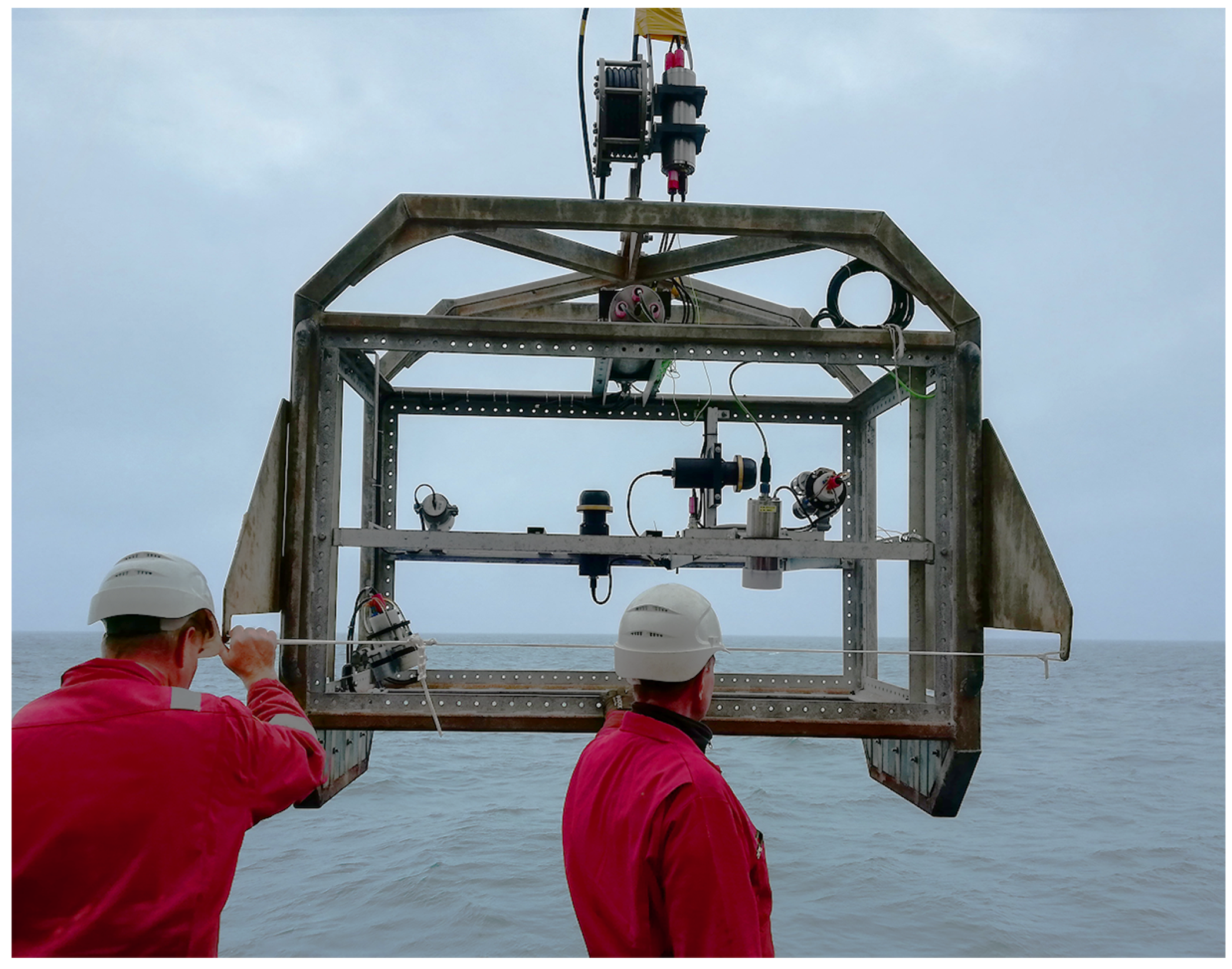
2.2. Multibeam Echosounder Data

For this survey, two MBESs were used, a Kongsberg EM 302 (Kongsberg Maritime, Kongsberg Gruppen ASA, Kongsberg, Norway) operating at 30 kHz, and a multi-spectral R2Sonic 2026 MBES (R2Sonic, Austin, TX, USA) operating at 90, 200, and 450 kHz. While the EM 302 was hull mounted, the R2Sonic was mounted on a pole on the side of the vessel. Because the R2Sonic was installed only for this survey, a patch test was performed prior to survey operations, using a shipwreck as a ground object. Location data were acquired with a global positioning system (GPS). Ship motion data were supplied by a motion reference unit (MRU). The GPS and MRU were both Kongsberg Seapath 360 (Kongsberg Seatex, Kongsberg Gruppen ASA, Trondheim, Norway) units. Just prior to this survey, the MRU system was replaced on the R/V Pelagia. During the survey, an incorrect MRU offset was discovered. In the Seapath software, an MRU yaw offset of 35°, towards starboard, was registered when the actual yaw offset of the MRU was 0.57° towards port. The ray-tracing error thus induced was corrected in post-processing. For the EM 302 data, there were no lingering artifacts after the correction. The R2Sonic operated with roll compensation enabled some of the data collected before the MRU offset error was corrected, falling outside the beam angles of −60° and 60° after data correction in post-processing. This does not affect the reliability of the results.
The bathymetry and backscatter data from all EM 302 survey lines were logged in the Kongsberg Seafloor Information System (SIS). For this sonar, the SIS software is used for both data logging and sonar control. The R2Sonic, on the other hand, was operated and controlled using R2Sonic’s Sonic Control software, while the data were logged in the Quality Positioning Services (QPS) (Quality Positioning Services, Zeist, The Netherlands) Qinsy software. Both bathymetry and backscatter data were collected. During survey operations, the R2Sonic was constantly monitored to ensure that the backscatter (BS) data would not be saturated (clipped). If there was a danger of saturated data, then the gain was adjusted as needed.
After the cruise, the data from both MBESs were cleaned. As a first step, all bathymetric outliers were removed using the QPS software Qimera. After this, Qimera’s automated data-cleaning algorithm was applied. The spikes in the 90-kHz data that resulted from the occasional interference from the 30-kHz sonar were removed. In post-processing, it was noticed that there had been some movement in the side pole from one survey to the next. This introduced lever-arm errors in the R2Sonic data, mainly related to the yaw and minimally to the roll of the R2Sonic MBES. These offset artifacts were also corrected, using Qimera and data from overlapping survey lines. The side pole was also not perfectly stiff. When there was wobble in the pole, it was very evident in the bathymetric data, especially in the outer beams. Unlike the error introduced between surveys, which was correctable, the errors induced by pole wobble were not correctable and the data containing these errors were deleted.
The GPS data had a vertical accuracy of 0.5 m. Because the MBES systems had better precision than 0.5 m, unpredictable vertical offsets in the bathymetry data were visible. Therefore, the vertical GPS data were disregarded, and the depth measured based on motion-corrected MBES data in conjunction with the known vessel draft. To overcome the effect of the tide, corrections were applied in Qimera from known tide data. After all corrections were applied, the EM 302 data were read into Qinsy and converted to ASCII format. The R2Sonic data were exported from Qimera in generic sensor format (gsf) from which the data were converted to the ASCII format. The ASCII data were read into MATLAB for further processing.
The backscatter (BS) data were corrected for spreading and frequency specific absorption. The corrections used ocean conditions as measured during the cruise based on conductivity, temperature, and pressure (CTD) data collected at the survey site. For the EM302 data, source levels applied during acquisition were used as outlined in [33]. For the R2Sonic data, receiver gain and source level corrections, which included directivity patterns, were applied in post-processing according to manufacturer recommendations. The backscatter values should be considered to be relative values, since absolute target strength calibrations were not performed. Ensonified area correction was performed for both sonars. For the R2Sonic data, an ensonified area correction was applied that took seafloor slopes into account, as was done in [34]. For the EM 302 data, it was necessary to first remove a flat seafloor based ensonified area correction that is implemented by Kongsberg. After this, slope and ensonified area corrections were applied as was done in [10,35] by the use of a digital terrain model based on the bathymetry from the MBES data. As part of the verification process, data that are not corrected for slope, receiver gain, and source levels are used; this is indicated when this is done.
The ARCs were computed by binning the beam angles from lowest to highest. The number of bins was determined by the number of beams of the MBES. In the case of the EM 302, there were 432 beams and in the case of the R2Sonic, 256 beams. All of the backscatter data within each angle bin were averaged per survey line. The average backscatter value per bin was then plotted as a function of beam angle to form the ARC.
For part of the analysis, the backscatter values are not plotted as a function of angle relative to the transducer, but of angle relative to North (Figure 3). This was done in order to obtain ARCs independent of sailing direction. This was only done for lines that were sailed in the East and West directions.

2.3. Video Data

In the troughs on either side of the Brown Bank videos of the seabed were collected. The video transects ranged in length from ~50 m to ~425 m (Figure 1). The NIOZ hopper camera (Figure 4) that was used is described well in [18,28]. It consists of a custom-made drop frame with a downward-facing HD video camera, an underwater light source (100 W), and two parallel green lasers (30 cm apart). The camera system was lowered to 0.5 m above the seabed, tethered to the vessel by a Kevlar cable with a glass fiber core allowing real-time video transfer.
In order to determine the orientation of the sand ripples on the seafloor from the video data, the following methodology was used. Based on the modeled tide data (Section 2.4), four video transects were selected, two of which were sailed when the tide was the strongest in the northern direction and two when the tide was the strongest towards the South. Of the selected transects, valid recordings were selected. Invalid recordings were those in which the seabed was not (clearly) visible, owing to particle clouds or motion, or in which at least one of the lasers was not visible. Of the valid recordings, seven images (still frames from the continuous video) were selected. Because the orientation of the video camera was not known, it was checked if the video camera was moving towards the top of the image, determined by observing the continuous video, or not. If not, the image was discarded and a replacement was found. For one of the transects, the video camera dominantly moved towards the bottom of the images. For this transect, images when the video camera moved towards the bottom of the image had to be used. Care was taken to use the correct offset to calculate the sand ripple orientation also for this transect. After the images were selected, the software ImageJ was used to draw seven lines on the images from crest to crest of the sand ripples. The statistics for line direction, relative to the image, and line length, relative to the laser points in the image were then computed in ImageJ. The mean compass direction of the sailed video transect was computed in ArcGIS. Both the calculations from ImageJ and from ArcGIS were then imported into the R software package and the ripple directions, relative to the images, were corrected using the mean transect direction, to have compass headings. The results indicated the compass direction that the lee-side of sand ripples were facing towards, in degrees from 0 to 360. In this case, 0° and 360° are both due North.
The lines in ImageJ used to calculate the orientation of the sand ripples were also used to determine the wave length L of the ripples. The known distance between the laser points in the image were used to scale the length of the lines drawn from crest to crest of the sand ripple to a physically meaningful length.

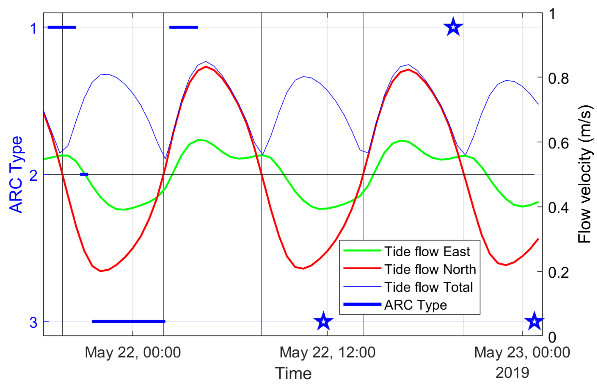
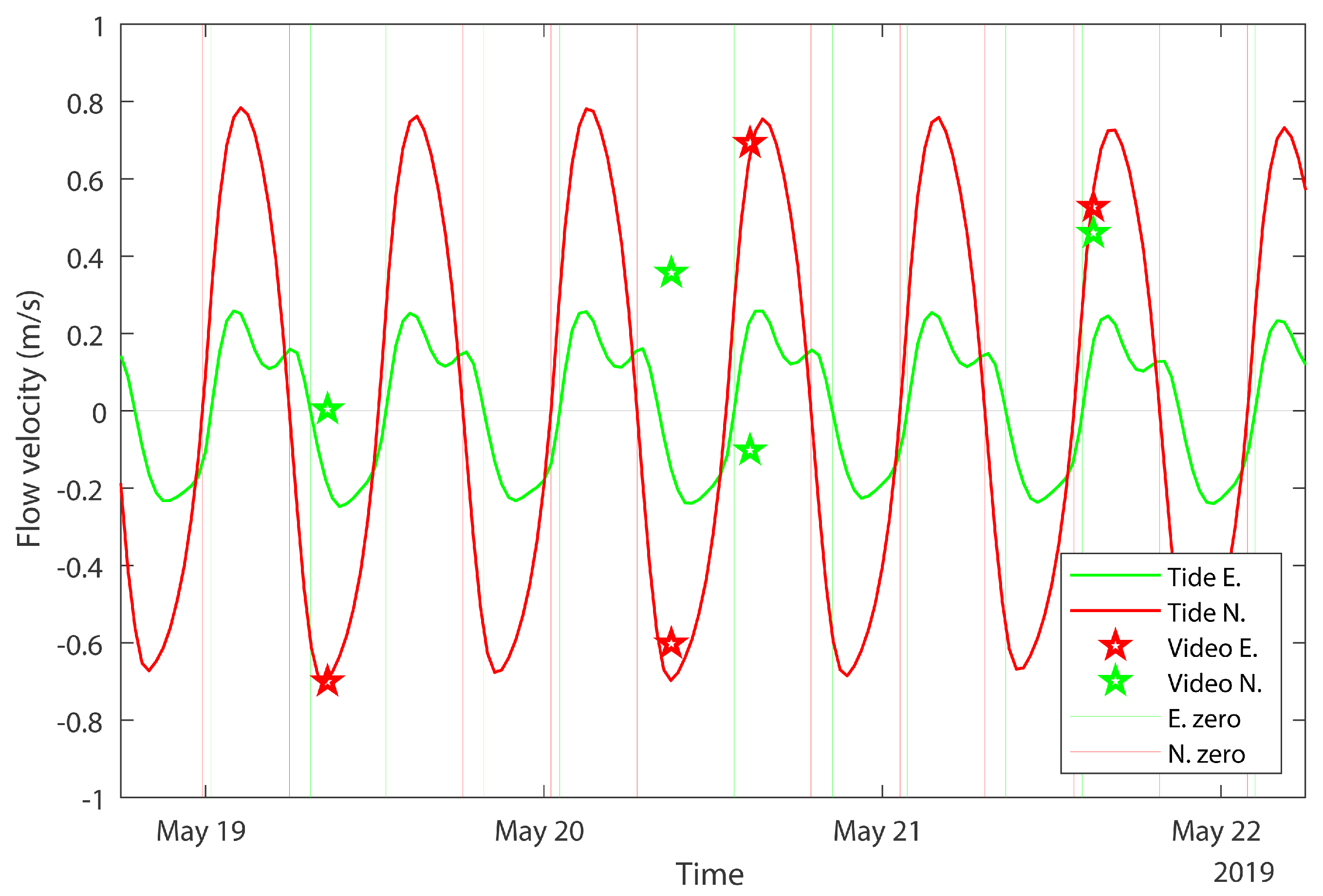
2.4. Tide Model Data

The tide data for this research were generated by the Dutch Continental Shelf Model, version 6 (dcsm v6) [37]. This model is maintained by Rijkswaterstaat and Deltares. The tidal model covers the Dutch Continental Shelf (DCS) from 48° to 62.25° N and 12° W to 13° E. The resolution is 1/8 degrees in longitude and 1/12 (~6.5–9.3 km and 9.25 km respectively) degrees in latitude. The model uses a set of eleven tide stations at the boundaries and space and time varying wind and pressure fields as boundary conditions and input parameters, respectively. A timestep of 10 min is used. The output is validated by the use of nineteen tide stations on the DCS that are not a part of the tide stations used for boundary conditions. The root mean square error in the model output is less than 0.094 m.
Modeled tidal data were retrieved for the center of the survey area, at 52.6167° N and 3.3167° E. The tidal flow velocities were obtained in the North and East directions in meters per second. These data were read into and used in MatLab for comparison to ARC types and the analyzed video data.

3. Results and Discussion

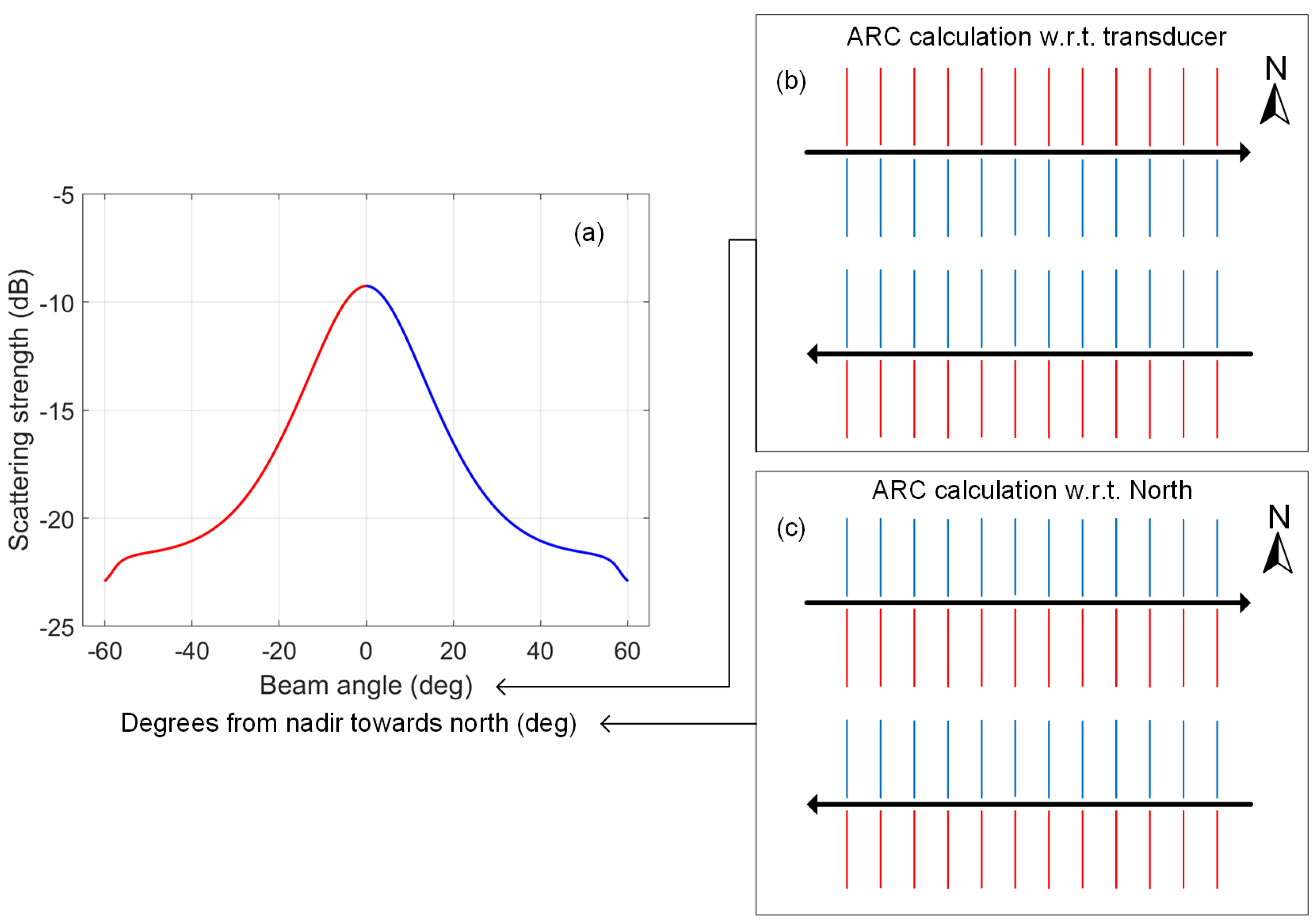
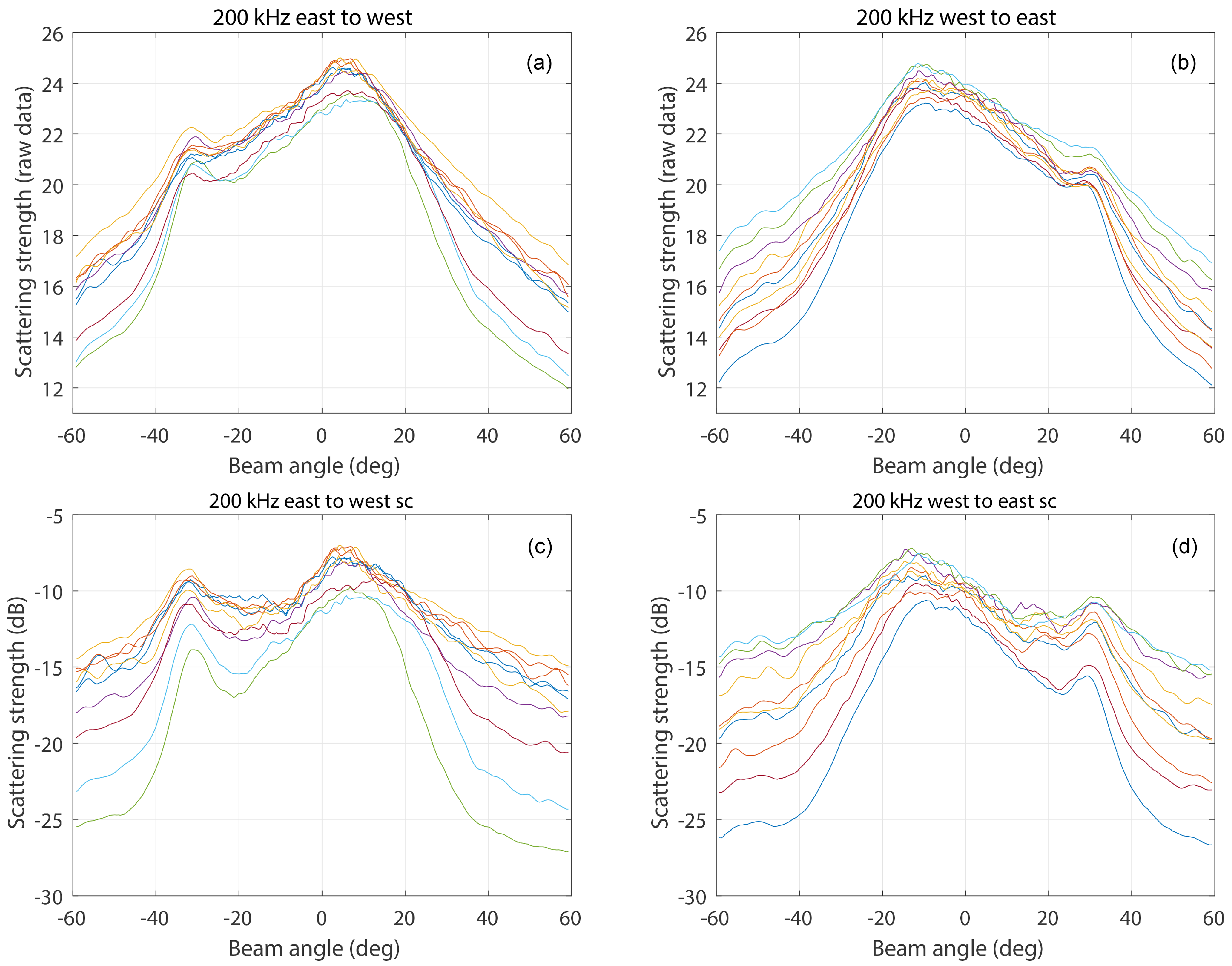
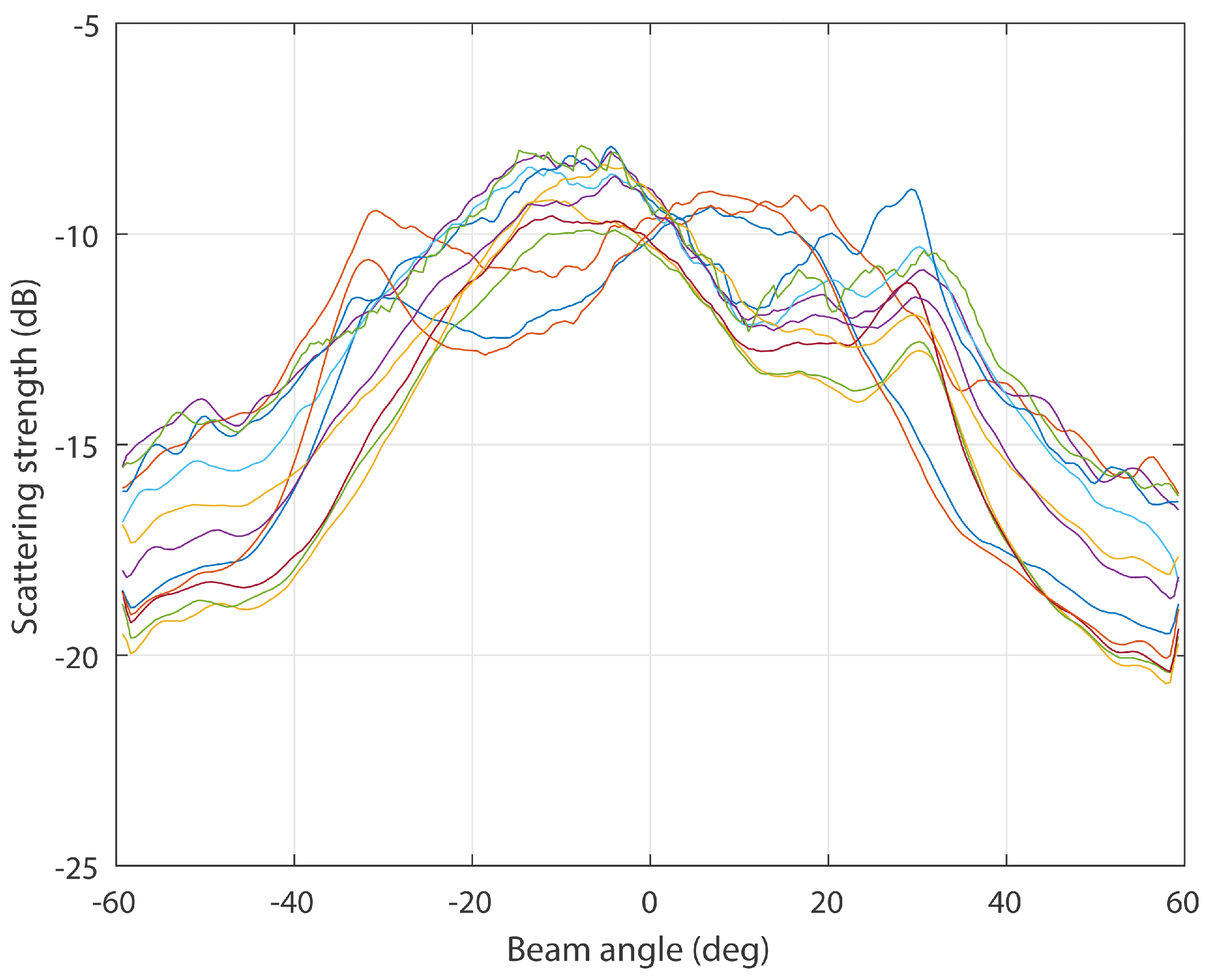
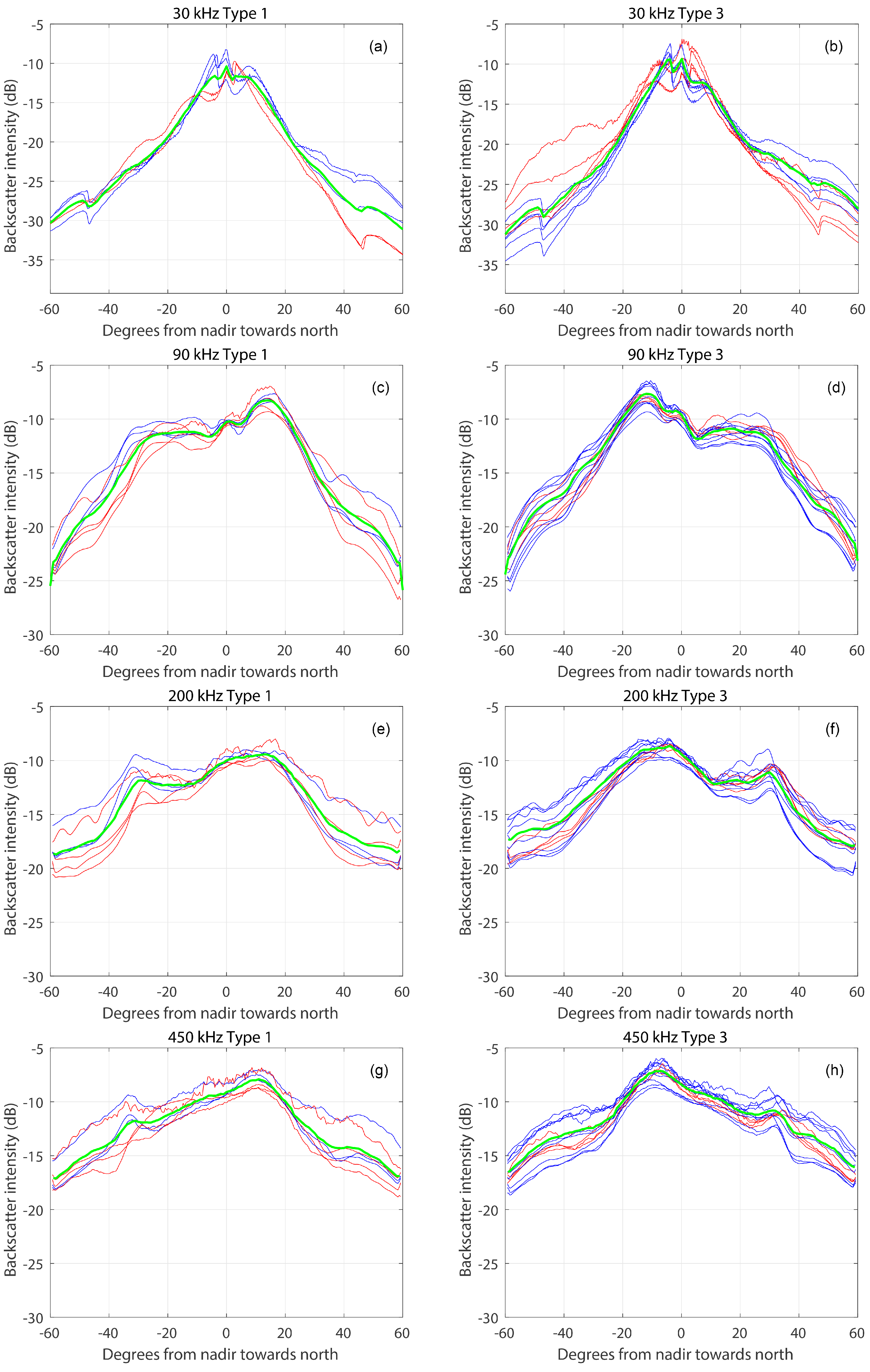
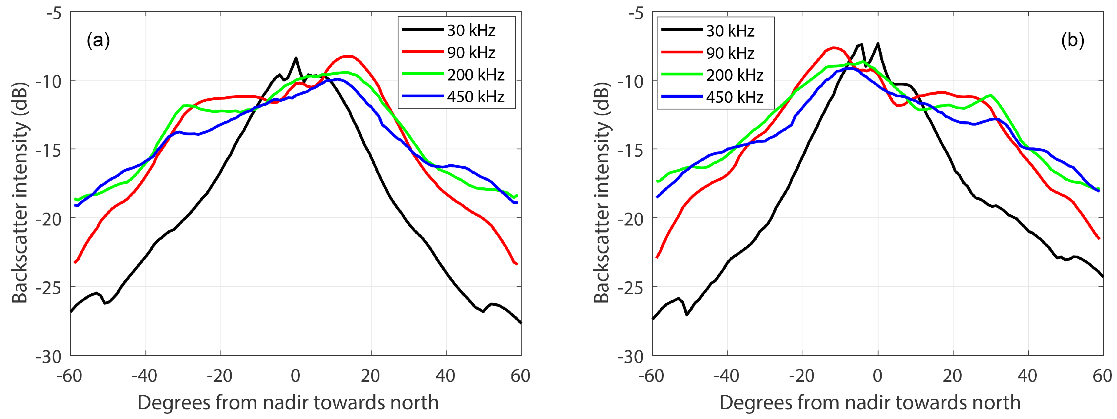
3.1. Angular-Response Curves

The method of computing the ARCs that was described in Section 2.2 is applied to the backscatter data from both the EM 302 and the R2Sonic multibeam echosounders (Figure 5). Backscatter data are often affected by errors induced by the mechanical properties of the transducer [11]. A characteristic of such errors is that they occur in all survey lines collected by the given sonar as long as the settings are kept constant. This means that the errors are independent of survey azimuths and sediment type. In the ARCs computed for all the different frequencies, there are a few examples of this. The clearest of these is at ±35° in the 450-kHz data (Figure 5d). This artifact is removed for the remainder of the figures by using the mean of the ARCs that were least affected by the sand ripples, interpolating the area of the dip with a line, and adding the difference between this line and the mean ARC to all the ARCs. The second most evident one is at 45° in the 30-kHz data (Figure 5a). For the purpose of the analysis of this paper, it was not necessary to remove this artifact.
The remaining artifacts are not present across all ARCs of a given frequency. The most noticeable case of this is in the ARCs of the 200-kHz data at ±30° (Figure 5c). At these angles, there is an increased backscatter intensity for some survey lines but not for others. A further analysis reveals that the lines with increased backscatter intensity were surveyed either from East to West or from West to East. Unlike the typical behavior of an ARC (Figure 3) [36], these ARCs do not peak at nadir but slightly off nadir. In addition, between 30° and 35°, there is a bump in the ARC. When the backscatter data are corrected both with respect to the seafloor slope and ensonified area, this behavior is still present (Figure 6c,d). The main difference in the slope corrected data is that the peaks in question are more widely distributed across more beam angles.
From Figure 5c, there is not a clear pattern, but some of the curves do show a mirrored pattern. An obvious hypothesis is that these inconsistencies are due to sailing direction. Comparing only specific lines to each other as in Figure 5, this hypothesis would be supported. However, a further investigation showed that the ARC pattern is not consistent when only one sailing direction is considered (Figure 7). To investigate the cause for this change, ARCs were plotted not as a function of beam angle relative to the transducer but relative to North (Figure 3 and Figure 8). This allowed the ARCs to be classified into four different types. ARCs which follow a typical pattern, with the peak at nadir (Figure 3), are referred to as Type 0. ARCs where the close-to-nadir peak is North of the transducer were called Type 1. When there were symmetrical peaks on either side of nadir, it was defined as Type 2 (only 1 survey line was Type 2). In addition, when the close-to-nadir peak was to the South, it was classified as Type 3. All of the East West lines that were sailed occurred between the evening of 21 May and the night of 23 May 2019. During the night of 21 May, acoustic surveys were carried out continuously for 11 h (ARC Type indicated by solid blue line in Figure 9). Then, on the morning and evening of 22 May, and the evening of May 23, single East–West survey lines were sailed (ARC type indicated by blue stars in Figure 9). It was found that the ARC type switched from Type 1 to Type 3 on six hour intervals (Figure 9). There was one instance of a Type 2 ARC on the evening of 22 May, at the point of a switch from Type 1 to Type 3. When the times of the switch in ARC Type are compared to the modeled tidal flow data, it is clear that the ARC Type change matches the switch in tidal flow direction (Figure 9).

3.2. Video Results

Video transects were selected and analyzed as explained in Section 2.3. An example of a selected image from the video footage is seen in Figure 10. The seafloor in this image is lit from the above right. Visible in this image is a seafloor with sand ripples. The gentle stoss-side slopes of these ripples and the lee-side slopes that are at the angle of repose (Angle of repose is the maximum slope, measured in degrees from the horizontal, at which loose solid material will remain in place without sliding.) (more on this in Section 3.3) are both clearly visible. In addition, shown are small yellow lines with a black dot in the middle. These are examples of the lines that were drawn in the software ImageJ to determine the ripple direction. The black arrow indicates the resulting estimate for the direction of these lines. Additionally, close to the top of the image are two greenish yellow dots. These are from the laser pointers of the camera system that are positioned exactly 30 cm apart.
The results from the analysis of the four video transects are shown in Table 1. This table gives the date and time, the mean orientation, mean length, and the associated standard deviations of the sand ripples for each transect. For the first two of these transects, S 1 4 and S 2 3 , the lee side of the sand ripple was facing South. For the last two transects, S 2 8 and S 2 4 , the lee side was facing North. The southward facing sand ripples had a length just over 10 cm. The North facing sand ripples had a length closer to 15 cm. The standard deviation for the orientation of the sand ripples was much greater in the first line than in the others, but still mainly facing South.
In order to compare this information to the modeled tidal flows, the data are superimposed on the tidal flow data in Figure 11. It is evident that the orientation of the sand ripple as derived from the camera measurements matches the tidal flow direction. This indicates that the ripple direction changes with the turning of the tide. In the East and West direction, for which the tidal flow is less strong, there is not a clear match with ripple directions (Figure 11).

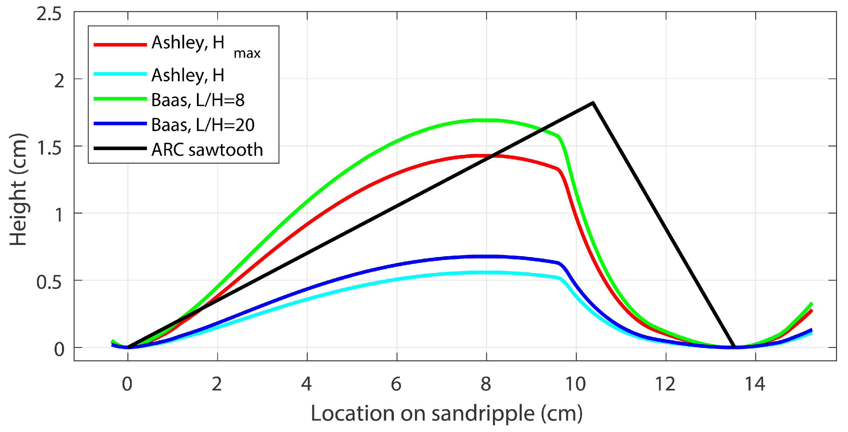
3.3. Quantifying Sand-Ripple Slopes on the Basis of Backscatter Data

Modeled results in [12] indicate that the angles at which the off-nadir peaks in the ARCs occur should match the angles of the slopes of the sand ripples. For the model, they used a “facet” model approach based on [38] for the close-to-nadir angles. For the oblique angles, Lambert’s law was used to describe the backscatter coefficient angle dependence. They simulated two seafloor ripple types. The first was a strictly sawtooth shaped sand ripple and the second a rectified-sine-shaped sand ripple. For the rectified-sine-shaped sand ripples, the resulting modeled ARC had peaks at the beam angle γ 0 , where γ 0 was also the maximum slope in the simulated sand ripples. For the simulated seafloor with a sawtooth-shaped sand ripple, the stoss and lee slopes had angles of γ 1 and γ 2 , respectively. For this simulated seafloor, there were peaks in the modeled ARCs at beam angles γ 1 and γ 2 . Based on this theory, it is expected that off-nadir peaks in the ARCs correspond to the slopes of the seafloor sand ripples.
The ARCs of Type 1 and Type 3 show peaks around ~10° and ~35° (Figure 12). These peaks are a little easier to recognize if the difference between the average ARC of either Type 1 or Type 3 and the average ARC of Type 0 is considered (Figure 13a,b Types 1 and 3, respectively). Based on the location of these peaks, sawtooth-shaped sand ripples with lee-side slopes of ~35° and stoss slopes of ~10 ° would be expected. Sawtooth-shaped sand ripples do indeed characterize the corresponding ground-truth video data. Furthermore, during the analysis of the video data, it was noticed that there were active avalanches on the lee side of the sand ripples. This video evidence implies that the lee-side slopes of the sand ripples are near the angle of repose. According to [39], this angle, for “water filled” sand, is between 15° and 30° and, for dry sand, it is 34°. The peaks in the ARCs (Figure 13) would indicate that the lee-side slopes are at ~35°. These values are somewhat higher than the “water filled” values given in [39] and up to values listed for dry sand. When the angle of repose was studied for non-uniform sediment in [40], the “in water” angle of repose for the same sediment mixtures was found to be higher than that of the “in air” angles. They listed angles of 38.29° (in air) to 40.96° (in water). These angles are higher than the ARCs would suggest, but this could be explained by the fact that [40] considered larger grain sizes than those found in the current study area. The match between the implied lee-side slopes indicated by the ARCs and the theoretical and experimental angles of repose from the literature supports the use of these acoustic methods to indicate the angles of sand ripples. It should be noted that this angle measurement does not come from the bathymetric measurements, but from the behavior of the backscatter at specific beam angles.
For the lee side of the sand ripple, we get an accurate independent estimate of the steepness of the slope, owing to the fact that avalanching occurs at a known angle of repose. For the stoss-side slopes, it is much harder to obtain independent information of the angles. From the video data, it is not possible to measure these angles. Furthermore, the surfaces of the box cores that were taken in this survey were deemed insufficient in size for accurate measurements. In addition, it is not known whether the surfaces remained intact in the grab taking process. As such, from the data in this research, we cannot conclusively say what the angles of the stoss sides of the sand ripples are. However, because of what we know from the lee slopes and the accuracy of their measurement, it is believed that the close-to-nadir peak in the ARCs is an accurate measure of the stoss slopes of the sand ripples. These slopes, thus, would be at ~10° (Figure 13).
To further investigate if these results are reasonably accurate, a strictly sawtooth-shaped sand ripple, with the angles derived from the ARCs for the stoss- and lee-side slopes, is superimposed on the schematic of typical sand ripples of the size found in the study area. This comparison depicts that the derived slopes match well with the expected slopes as reported in the literature (Figure 14). Using the stoss- and lee-side angles as 10° and 35° would give a vertical form index of 7.5 when assuming a strictly saw-tooth shape. Given that the sand ripples are unlikely to have a perfect sawtooth form, a larger vertical form index is expected, which would match well with the values given by [32]. We thus conclude that both the stoss- and lee-side angles of 10° and 35° are reasonable values for the sand ripples in the study area.

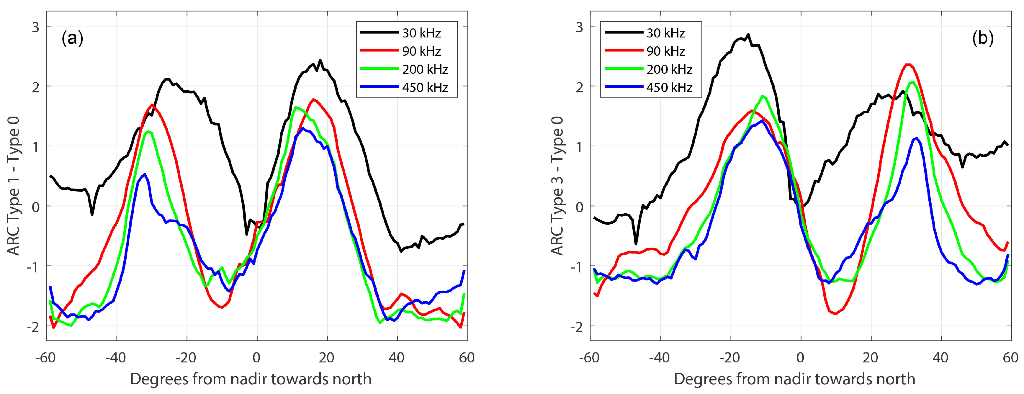
3.4. Sand-Ripple Effects on Different Frequencies

We now analyze how the sand ripples affect different frequencies. For each frequency, there are clear peaks around ~10° and ~35° (Figure 12, Figure 13 and Figure 15). For the peaks corresponding to the steep lee slopes of the sand ripples lower frequencies generally correspond to higher peaks, with a difference as large as 1.5 dB between the frequencies. For lower frequencies, the peaks are also closer to nadir by up to 8°. For the peaks corresponding to the stoss-side slopes of the sand ripples, no trend for the increasing or decreasing frequencies was found. However, the 200-kHz peak was at 11° and the 30-kHz peak was at 15°, a difference of 4°. The 450-kHz peaks were between the 200-kHz and 90-kHz peaks.
According to [12], different frequencies were similarly affected by sand ripples. They used 300 kHz and 100 kHz, although they did not show the 100-kHz results. They also claimed that angles higher than 40° would not be affected, which is confirmed by our results for frequencies between 90 kHz and 450 kHz. For the 30-kHz data, however, angles higher than 40° were also affected. Furthermore, the effect of the lee slopes was spread over more angles in the case of the 30 kHz data. We hypothesize that this is because the flanks of the lee side slopes are shorter than the 5 cm signal wave length at 30 kHz. As such, these flanks no longer follow a specular scattering regime as assumed by the “facet” model [12], but more of a roughness scattering regime.
For each of the frequencies considered here, the extent of the beam footprint should not have a significant effect on the backscatter response at the angles of the sand ripple slopes. Even in the case of the 450-kHz data, the beam footprint in the shallowest water still had an across-track extent covering more than one sand ripple (Figure 16). Additionally, the fact that the lee slopes of the sand ripples affected more angles in the 30-kHz data were not due to a difference in beam footprint. The 90-kHz beam footprint of the R2Sonic had a larger extent than that of the 30-kHz EM 302, and the data were not affected over as many angles.

3.5. Implications for Backscatter-Based Sediment Classification

Because backscatter is affected by sand ripples, the results in this paper also have implications for the outcome from a number of different types of backscatter-based classification algorithms [41]. These include algorithms where the classification is based on parameter estimation by the fitting of curves to the ARCs [42], algorithms where backscatter intensities are considered per beam angle [10,13], and algorithms where a correction curve for the mechanical properties of the transducer is calculated [11] using survey data tainted by the presence of undetected sand ripples.
This is not to say that such algorithms cannot be used in sandy areas with high-velocity tidal currents. Algorithms based on ARC fitting may need to be adjusted in such areas—for example, by giving the angles that are the most likely to be affected less weight when fitting the curves. Algorithms considering single beam angles should avoid using beam angles that are affected. According to [12] and our results for frequencies 90 kHz and higher, angles farther from nadir than 40° should not be affected by these types of seabed features. As for the calculation of correction curves for the mechanical properties of the transducer, this research and that of [12] strongly suggest that data from a sandy seafloor area with high current velocities should not be used to calculate the correction curves.
It is common to correct backscatter values for the seafloor slope [10,11,35]. The slope correction is performed by using the bathymetry that comes from the same data as the backscatter. As is clear from the case in this research, see Figure 6, and is also from [12], the seafloor features that affect the backscatter data here are smaller than the resolution of the MBES bathymetry. As such, for these features, a slope correction cannot be carried out. For future work, it would be worth examining if new developments, like R2Sonic’s Ultra High Density (UHD) settings, could resolve these seafloor features. If that is possible, then a slope or other correction may also be within reach for these seafloor features.
However, if a survey was designed and carried out specifically to detect sand ripples, with bathymetry, of the size found here, by mounting an MBES on a remotely operated vehicle (ROV), using high enough frequencies, and slow sailing speeds, the effect encountered here could still not be ruled out, although the effect would then be caused by proportionally smaller ripples. On the flip side, it is also possible that mega ripples, which are easily detected in the bathymetry in this survey, would similarly effect the backscatter of MBESs operating in the deep oceans with low frequencies.

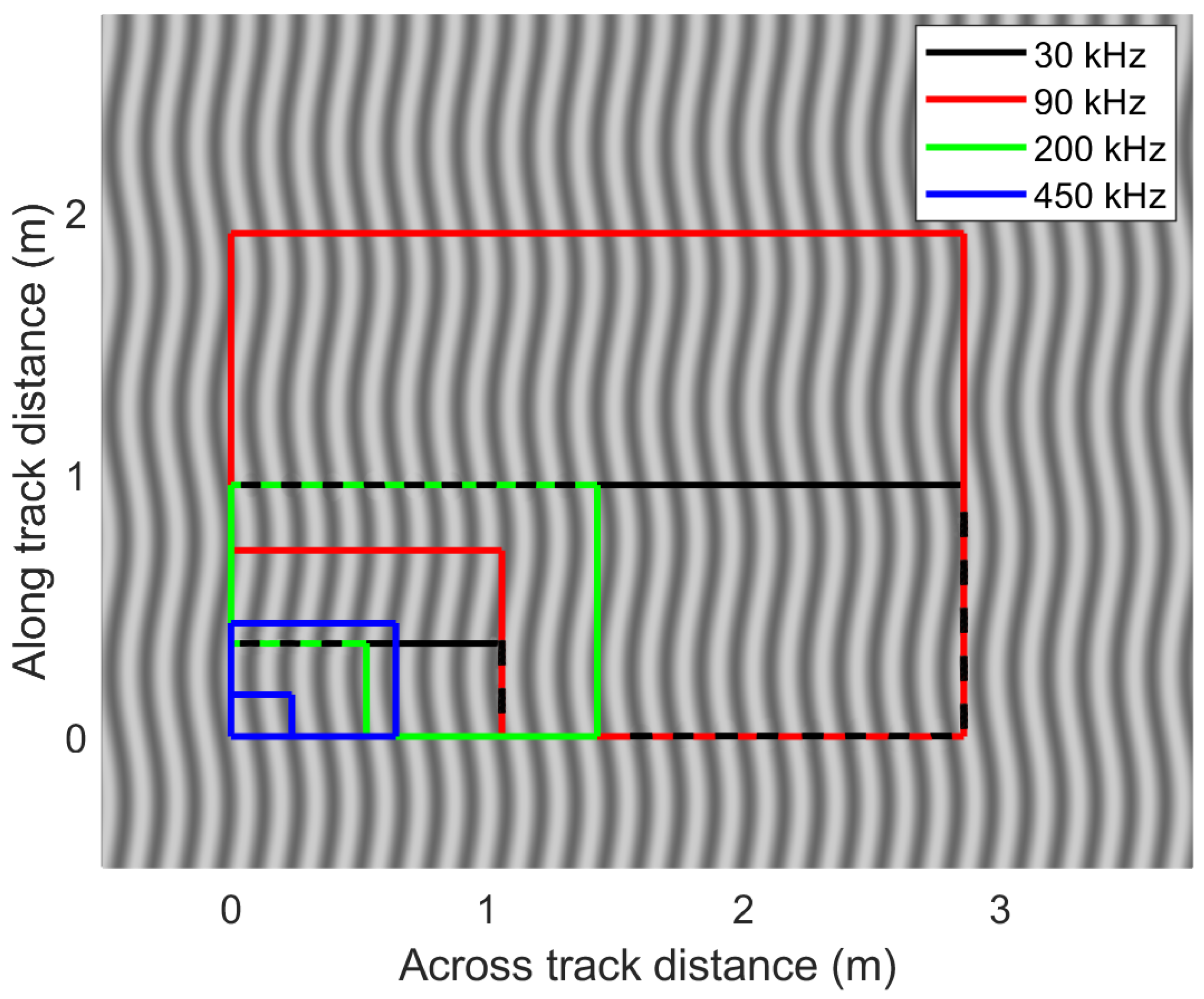
3.6. Sand Ripple Detection over Large Geographical Areas

The final and most important matter that this study shows, which would be difficult to show by another methodology, are the large geographical scales at which the sand ripples change. Tidal ridges [23,24], sand waves [26,43,44], and megaripples [27,45,46] have been studied at great length over the years, using grab samples, MBES bathymetry, SSS data, and video data, along with sediment transport models. Although these methods are effective for large seafloor structures, it would be challenging to use these in ocean environments for sand ripples. This is due to the small scale of sand ripples and the difficulty of detecting them. Using video systems would be an effective method to study sand ripples in the ocean. However, detailed experiments, for the most part, have been carried out in the lab. SSS imagery may also be able to show at least the presence of these sand ripples, if operated correctly, but it is unknown if the orientation of the sand ripples could be determined [15]. The use of the MBES backscatter, as an acoustic instrument, allows the large scale study of the behavior of the sand ripples in ways that the other methodologies are unable to do. The results of the backscatter data in this study conclusively show that the orientation of the sand ripples changes to opposite directions across many kilometers of seafloor in a matter of hours.
The results from this research further apply to seafloor classification and monitoring efforts over most of the sandy southern portion of the North Sea. They also apply to many other areas, including places such as the Outer Bristol Channel off the Welsh coast [47], in the western part of the Barents Sea [48], small parts of the Cook Strait [42], and large parts of the continental shelf of the East China Sea and South China Sea [49], to name just a few. All of these areas are sandy areas with a potential for high velocity currents.

4. Summary and Conclusions

In this paper, we found that small-scale repeating seafloor structures (sand ripples) have a profound impact on ARCs. These ARCs are calculated from MBES backscatter data. Visible in these ARCs are unexpected off-nadir peaks. These patterns were influenced by the survey azimuth, but not consistent when the survey azimuth was held constant. It was found that the pattern switched on the same time intervals as the switch of the tidal flow direction. Lurton et al. [12] found similar survey-azimuth-dependent backscatter patterns. We further show that, even for the same area of seafloor and a constant survey azimuth, backscatter results can differ in time. Video data confirmed that the switch in ARC pattern matched an orientation switch in sand ripples on the seafloor. These results have implications for several currently used classification algorithms. In particular, care must be taken that it is not seafloor morphology, rather than seafloor sediment composition that is being characterized when performing backscatter-based seafloor characterization.
We suggest that the pattern in the ARCs is useful as a diagnostic tool. Firstly, the off-nadir peaks in the ARCs indicate the slope angles of the sand ripples. The slopes indicated by the ARCs in this research matched well with typical sand ripple slopes from the literature. From the two angles, the avalanching observed for the lee-side ripples in the video data allowed the use of the known angle of repose for sand in water to be compared with the angles indicated from the ARC patterns. The indicated slopes of the stoss side of the sand ripples are harder to validate.
Another strength of this research is that we had four frequencies of MBES data from the same areas of the seafloor, all gathered at the same time. This was possible by operating two different MBESs simultaneously. The first of these operated at 30 kHz and the other operated at multiple frequencies, 90, 200, and 450 kHz. All of these frequencies were affected similarly by the gentle stoss slopes of the sand ripples. This was evident by similar peaks in the ARCs that matched with the angles expected for these slopes. Furthermore, the ARCs were affected at different angles, with the higher frequencies having a peak at higher beam angles. In addition, for lower frequencies, the ARC peaks were more widely distributed. In the case of the 30-kHz data, beam angles beyond 40° were also affected. For the sand ripples encountered in this research, the 200-kHz data seemed to indicate the sand ripples the best. As such, if a survey was designed with the purpose of detecting sand ripples and only one frequency was available, then 200 kHz would be a good choice to use.
The most important result of this research is that we show a clear link between ARC pattern and sand ripple orientation on the seafloor. This was confirmed by the use of both video ground-truth data and modeled tide-flow data. These patterns could thus be predicted over spatial scales of kilometers. The use of MBES bathymetry would have failed to yield this result, owing to the insufficient resolution of the bathymetry data. Using our methodology, we were able to show that the top centimeter of the seafloor undergoes a complete transformation every six hours in this part of the North Sea. The capability to make such predictions from acoustic data makes these types of measurements an invaluable tool for ocean monitoring.

Author Contributions

Conceptualization, L.K., K.J.v.d.R., M.S., and D.G.S.; methodology, L.K., K.J.v.d.R., and M.S.; software, L.K., and K.J.v.d.R.; formal analysis, L.K., K.J.v.d.R., and M.S.; investigation, L.K. and K.J.v.d.R.; resources, L.K., K.J.v.d.R., T.Y., L.L.G., P.M.J.H., H.O., M.S., and D.G.S.; data curation, L.K. and K.J.v.d.R.; writing—original draft preparation, L.K., K.J.v.d.R., P.M.J.H., H.O., and M.S.; writing—review and editing, L.K., K.J.v.d.R., S.M., T.Y., L.L.G., P.M.J.H., H.O., M.S., and D.G.S.; visualization, L.K., K.J.v.d.R., and M.S.; supervision, T.Y., L.L.G., P.M.J.H., H.O., M.S., and D.G.S.; project administration, L.K., K.J.v.d.R., S.M., T.Y., L.L.G., P.M.J.H., H.O., M.S., and D.G.S.; funding acquisition, P.M.J.H., H.O., M.S., and D.G.S. All authors have read and agreed to the published version of the manuscript.

Funding

This research is part of the multidisciplinary research project DISCLOSE. DISCLOSE is a joint venture of the Delft University of Technology, the University of Groningen, the Royal Netherlands Institute for Sea Research, as well as the North Sea Foundation. DISCLOSE is funded by the Gieskes Strijbis Fonds.

Acknowledgments

The authors would like to thank the crew of the R/V Pelagia for their hard work during the cruise to gather the research data. Jip Vrooman (then from the North Sea Foundation) is acknowledged for organizing the data collection cruise. Rian Brak and Jeroen Daams from QPS are thanked for their role in setting up the acquisition system for the R2Sonic MBES. QPS is also thanked for supplying the Qinsy, Qimera, and Fledermaus software licenses that were used during the acquisition and processing of the MBES data. Raoul Michels and Elisabeth van Spelden are thanked for their nights of work during survey operations. Marc Philippart and Simon Bicknese from Rijkswaterstaat were vital in supplying the tide model data. Finally, Leendert Dorst and Daniëlle van Kuijk of the Hydrographic Service within the Royal Netherlands Navy were key in making full-coverage high-resolution bathymetric data available from the Brown Bank.

Conflicts of Interest

The authors declare no conflict of interest. The funders had no role in the design of the study; in the collection, analyses, or interpretation of data; in the writing of the manuscript; or in the decision to publish the results.

Abbreviations

The following abbreviations are used in this manuscript:
ARCAngular-response curve
BSBackscatter
cmCentimeter
CTDConductivity temperature, and pressure
dBDecibel
DCSDutch continental shelf
DTMDigital terrain model
GPSGlobal positioning system
gsfGeneric sensor format
MBESMultibeam echosounder
mMeter
mmMillimeter
MRUMotion reference unit
MSFDMarine Strategy Framework Directive
NIOZRoyal Netherlands Institute for Sea Research
QPSQuality positioning services
ROVRemotely operated vehicle
SISSeafloor information system
SSSSide scan sonar

References

  1. Halpern, B.S.; Walbridge, S.; Selkoe, K.A.; Kappel, C.V.; Micheli, F.; D’Agrosa, C.; Bruno, J.F.; Casey, K.S.; Ebert, C.; Fox, H.E.; et al. A global map of human impact on marine ecosystems. Science 2008, 319, 948–952. [Google Scholar] [CrossRef] [PubMed] [Green Version]
  2. Glegg, G.; Jefferson, R.; Fletcher, S. Marine governance in the English Channel (La Manche): Linking science and management. Mar. Pollut. Bull. 2015, 95, 707–718. [Google Scholar] [CrossRef] [PubMed] [Green Version]
  3. Busiest Shipping Lane. Online, Guinness World Records. 2020. Available online: https://www.guinnessworldrecords.com/world-records/busiest-shipping-lane (accessed on 8 December 2020).
  4. Amoroso, R.O.; Pitcher, C.R.; Rijnsdorp, A.D.; McConnaughey, R.A.; Parma, A.M.; Suuronen, P.; Eigaard, O.R.; Bastardie, F.; Hintzen, N.T.; Althaus, F.; et al. Bottom trawl fishing footprints on the world’s continental shelves. Proc. Natl. Acad. Sci. USA 2018, 115, E10275–E10282. [Google Scholar] [CrossRef] [PubMed] [Green Version]
  5. Van der Reijden, K.J.; Hintzen, N.T.; Govers, L.L.; Rijnsdorp, A.D.; Olff, H. North Sea demersal fisheries prefer specific benthic habitats. PLoS ONE 2018, 13, e0208338. [Google Scholar] [CrossRef] [PubMed] [Green Version]
  6. Rice, J.; Arvanitidis, C.; Borja, A.; Frid, C.; Hiddink, J.G.; Krause, J.; Lorance, P.; Ragnarsson, S.Á.; Sköld, M.; Trabucco, B.; et al. Indicators for sea-floor integrity under the European Marine Strategy Framework Directive. Ecol. Indic. 2012, 12, 174–184. [Google Scholar] [CrossRef] [Green Version]
  7. Snellen, M.; Gaida, T.C.; Koop, L.; Alevizos, E.; Simons, D.G. Performance of Multibeam Echosounder Backscatter-Based Classification for Monitoring Sediment Distributions Using Multitemporal Large-Scale Ocean Data Sets. IEEE J. Ocean. Eng. 2019, 44, 142–155. [Google Scholar] [CrossRef] [Green Version]
  8. Glenn, M.F. Introducing an operational multi-beam array sonar. Int. Hydrogr. Rev. 1970. [Google Scholar]
  9. Lamarche, G.; Lurton, X. Recommendations for improved and coherent acquisition and processing of backscatter data from seafloor-mapping sonars. Mar. Geophys. Res. 2018, 39, 5–22. [Google Scholar] [CrossRef] [Green Version]
  10. Koop, L.; Amiri-Simkooei, A.; J van der Reijden, K.; O’Flynn, S.; Snellen, M.; G Simons, D. Seafloor Classification in a Sand Wave Environment on the Dutch Continental Shelf Using Multibeam Echosounder Backscatter Data. Geosciences 2019, 9, 142. [Google Scholar] [CrossRef] [Green Version]
  11. Schimel, A.C.; Beaudoin, J.; Parnum, I.M.; Le Bas, T.; Schmidt, V.; Keith, G.; Ierodiaconou, D. Multibeam sonar backscatter data processing. Mar. Geophys. Res. 2018, 39, 121–137. [Google Scholar] [CrossRef]
  12. Lurton, X.; Eleftherakis, D.; Augustin, J.M. Analysis of seafloor backscatter strength dependence on the survey azimuth using multibeam echosounder data. Mar. Geophys. Res. 2018, 39, 183–203. [Google Scholar] [CrossRef]
  13. Simons, D.G.; Snellen, M. A Bayesian approach to seafloor classification using multi-beam echo-sounder backscatter data. Appl. Acoust. 2009, 70, 1258–1268. [Google Scholar] [CrossRef]
  14. Montereale-Gavazzi, G.; Roche, M.; Degrendele, K.; Lurton, X.; Terseleer, N.; Baeye, M.; Francken, F.; Van Lancker, V. Insights into the short-term tidal variability of multibeam backscatter from field experiments on different seafloor types. Geosciences 2019, 9, 34. [Google Scholar] [CrossRef]
  15. Elston, G.R.; Bell, J.M. Pseudospectral time-domain modeling of non-Rayleigh reverberation: Synthesis and statistical analysis of a sidescan sonar image of sand ripples. IEEE J. Ocean. Eng. 2004, 29, 317–329. [Google Scholar] [CrossRef]
  16. Von Rönn, G.A.; Schwarzer, K.; Reimers, H.C.; Winter, C. Limitations of Boulder Detection in Shallow Water Habitats Using High-Resolution Sidescan Sonar Images. Geosciences 2019, 9, 390. [Google Scholar] [CrossRef] [Green Version]
  17. Hansen, R.E. Mapping the ocean floor in extreme resolution using interferometric synthetic aperture sonar. In Proceedings of the Meetings on Acoustics ICU. Acoustical Society of America, Aachen, Germany, 9–13 September 2019; Volume 38, p. 055003. [Google Scholar]
  18. Damveld, J.H.; Van Der Reijden, K.; Cheng, C.; Koop, L.; Haaksma, L.; Walsh, C.; Soetaert, K.; Borsje, B.W.; Govers, L.; Roos, P.; et al. Video transects reveal that tidal sand waves affect the spatial distribution of benthic organisms and sand ripples. Geophys. Res. Lett. 2018, 45, 11–837. [Google Scholar] [CrossRef] [Green Version]
  19. Ferrini, V.L.; Flood, R.D. The effects of fine-scale surface roughness and grain size on 300 kHz multibeam backscatter intensity in sandy marine sedimentary environments. Mar. Geol. 2006, 228, 153–172. [Google Scholar] [CrossRef]
  20. Van Lancker, V.; Jacobs, P. The dynamical behaviour of shallow-marine dunes. In Proceedings of the International Workshop on Marine Sandwave Dynamics, Lille, France, 23–24 March 2000; pp. 213–220. [Google Scholar]
  21. Walgreen, M.; De Swart, H.E.; Calvete, D. A model for grain-size sorting over tidal sand ridges. Ocean. Dyn. 2004, 54, 374–384. [Google Scholar] [CrossRef]
  22. Svenson, C.; Ernstsen, V.B.; Winter, C.; Bartholomä, A.; Hebbeln, D. Tide-driven sediment variations on a large compound dune in the Jade tidal inlet channel, Southeastern North Sea. J. Coast. Res. 2009, 361–365. [Google Scholar]
  23. Van Dijk, T.A.; van Dalfsen, J.A.; Van Lancker, V.; van Overmeeren, R.A.; van Heteren, S.; Doornenbal, P.J. Benthic habitat variations over tidal ridges, North Sea, The Netherlands. In Seafloor Geomorphology as Benthic Habitat; Elsevier: Amsterdam, The Netherlands, 2012; pp. 241–249. [Google Scholar]
  24. Knaapen, M.A. Sandbank occurrence on the Dutch continental shelf in the North Sea. Geo-Mar. Lett. 2009, 29, 17–24. [Google Scholar] [CrossRef]
  25. Van Dijk, T.A.; Lindenbergh, R.C.; Egberts, P.J. Separating bathymetric data representing multiscale rhythmic bed forms: A geostatistical and spectral method compared. J. Geophys. Res. Earth Surf. 2008, 113. [Google Scholar] [CrossRef]
  26. Van Oyen, T.; Blondeaux, P.; Van den Eynde, D. Sediment sorting along tidal sand waves: A comparison between field observations and theoretical predictions. Cont. Shelf Res. 2013, 63, 23–33. [Google Scholar] [CrossRef]
  27. Van Der Reijden, K.J.; Koop, L.; O’flynn, S.; Garcia, S.; Bos, O.; Van Sluis, C.; Maaholm, D.J.; Herman, P.M.; Simons, D.G.; Olff, H. Discovery of Sabellaria spinulosa reefs in an intensively fished area of the Dutch Continental Shelf, North Sea. J. Sea Res. 2019, 144, 85–94. [Google Scholar] [CrossRef] [Green Version]
  28. Biber, M.F.; Duineveld, G.C.; Lavaleye, M.S.; Davies, A.J.; Bergman, M.J.; van den Beld, I.M. Investigating the association of fish abundance and biomass with cold-water corals in the deep Northeast Atlantic Ocean using a generalised linear modelling approach. Deep. Sea Res. Part II Top. Stud. Oceanogr. 2014, 99, 134–145. [Google Scholar] [CrossRef]
  29. Herman, P.; Beauchard, O.; van Duren, L. De staat van de Noordzee. Noordzeedagen. 2014. Available online: https://www.noordzeedagen.nl/nl/noordzeedagen/Vorige-edities/Noordzeedagen-2014-1/Thema-Leven-met-een-veranderende-Noordzee-Horizon-2050./De-staat-van-de-Noordzee.htm (accessed on 8 December 2020).
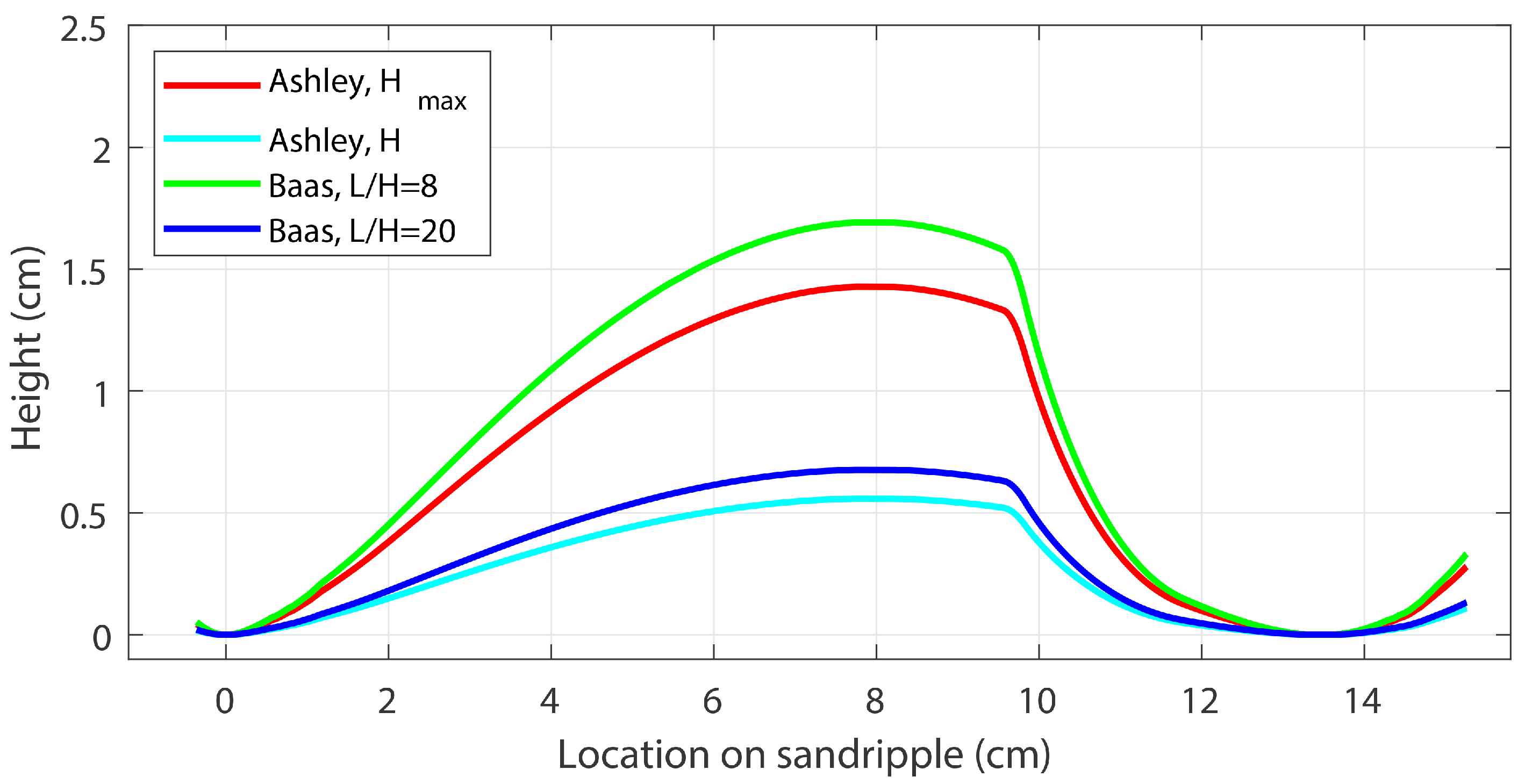
  30. Ashley, G.M. Classification of large-scale subaqueous bedforms; a new look at an old problem. J. Sediment. Res. 1990, 60, 160–172. [Google Scholar]
  31. Flemming, B. Zur klassifikation subaquatischer, strömungstransversaler Transportkörper. Boch. Geol. Und Geotech. Arb. 1988, 29. [Google Scholar]
  32. Baas, J.H. Ripple, ripple mark, ripple structure. Sedimentology 1978, 921–925. [Google Scholar]
  33. Hammerstad, E. EM Technical Note: Backscattering and Seabed Image Reflectivity. In Horten, Norway: Kongsberg Maritime AS. 2000. Available online: https://www.kongsberg.com/globalassets/maritime/km-products/product-documents/em_technical_note_web_backscatteringseabedimagereflectivity.pdf (accessed on 8 December 2020).
  34. Gaida, T.; Tengku Ali, T.; Snellen, M.; Amiri-Simkooei, A.; van Dijk, T.; Simons, D. A Multispectral Bayesian Classification Method for Increased Acoustic Discrimination of Seabed Sediments Using Multi-Frequency Multibeam Backscatter Data. Geosciences 2018, 8, 455. [Google Scholar] [CrossRef] [Green Version]
  35. Amiri-Simkooei, A.; Snellen, M.; Simons, D.G. Riverbed sediment classification using multi-beam echo-sounder backscatter data. J. Acoust. Soc. Am. 2009, 126, 1724–1738. [Google Scholar] [CrossRef] [PubMed]
  36. Applied Physics Laboratory, University of Washington. APL-UW High-Frequency Ocean Environmental Acoustic Models Handbook; Technical Report APL-UW TR9407; Applied Physics Laboratory, University of Washington: Seattle, WA, USA, 1994. [Google Scholar]
  37. Rijkswaterstaat and Deltares. Dutch Continental Shelf Model Modelbeschrijving. 2009. Available online: https://www.helpdeskwater.nl/publish/pages/131723/dcsm-v5.pdf (accessed on 8 December 2020).
  38. Tang, D.; Williams, K.L.; Thorsos, E.I. Utilizing high-frequency acoustic backscatter to estimate bottom sand ripple parameters. IEEE J. Ocean. Eng. 2009, 34, 431–443. [Google Scholar] [CrossRef]
  39. Al-Hashemi, H.M.B.; Al-Amoudi, O.S.B. A review on the angle of repose of granular materials. Powder Technol. 2018, 330, 397–417. [Google Scholar] [CrossRef]
  40. Yang, F.G.; Liu, X.N.; Yang, K.J.; Cao, S.Y. Study on the angle of repose of nonuniform sediment. J. Hydrodyn. 2009, 21, 685–691. [Google Scholar] [CrossRef]
  41. Brown, C.J.; Smith, S.J.; Lawton, P.; Anderson, J.T. Benthic habitat mapping: A review of progress towards improved understanding of the spatial ecology of the seafloor using acoustic techniques. Estuarine Coast. Shelf Sci. 2011, 92, 502–520. [Google Scholar] [CrossRef]
  42. Lamarche, G.; Lurton, X.; Verdier, A.L.; Augustin, J.M. Quantitative characterisation of seafloor substrate and bedforms using advanced processing of multibeam backscatter—Application to Cook Strait, New Zealand. Cont. Shelf Res. 2011, 31, S93–S109. [Google Scholar] [CrossRef] [Green Version]
  43. Knaapen, M. Sandwave migration predictor based on shape information. J. Geophys. Res. Earth Surf. 2005, 110. [Google Scholar] [CrossRef] [Green Version]
  44. Nemeth, A. Modelling Offshore Sand Waves. 2003. Available online: https://research.utwente.nl/en/publications/modelling-offshore-sand-waves (accessed on 8 December 2020).
  45. Idier, D.; Ehrhold, A.; Garlan, T. Morphodynamique d’une dune sous-marine du détroît du pas de Calais. C. R. Geosci. 2002, 334, 1079–1085. [Google Scholar] [CrossRef]
  46. Lindenbergh, R.C.; van Dijk, T.A.; Egberts, P.J. Separating bedforms of different scales in echo sounding data. In Coastal Dynamics 2005: State of the Practice; ASCE Library: Barcelona, Spain, 2006; pp. 1–14. [Google Scholar]
  47. James, J.C.; Mackie, A.S.; Rees, E.I.S.; Darbyshire, T. Sand wave field: The OBel Sands, Bristol Channel, UK. In Seafloor Geomorphology as Benthic Habitat; Elsevier: Amsterdam, The Netherlands, 2012; pp. 227–239. [Google Scholar]
  48. Aird, P. Chapter 4—Deepwater Metocean Environments. In Deepwater Drilling; Aird, P., Ed.; Gulf Professional Publishing: Houston, TX, USA, 2019; pp. 111–164. [Google Scholar] [CrossRef]
  49. Yincan, Y. Chapter 15—Development Laws of Geological Hazards and Hazard Geology Regionalization of China Seas. In Marine Geo-Hazards in China; Elsevier: Amsterdam, The Netherlands, 2017; pp. 657–687. [Google Scholar] [CrossRef]
Figure 1. (a) Bathymetry of the Brown Bank area with black lines indicating survey lines, red lines indicating the location of video transects, and black arrows indicating the tidal ridge and superimposed sand waves; (b) geographic setting of the research site at the Brown Bank, color indicates bathymetry.
Geosciences 10 00495 g001
Figure 2. Schematic structure of the sandripples expected in the survey area deduced from the ripple wavelength.
Geosciences 10 00495 g002
Figure 3. Schematic of the different ways the ARCs are calculated throughout the paper. (a) backscatter strength as a function of beam angle as calculated by the UW-APL model [36] at 90 kHz for medium sand. The different colors for the negative beam angles and positive beam angles indicate what data are used for the calculation of the ARCs as indicated in sub-figures (b,c); (b) a schematic of the data typically used to calculate ARCs. The black arrow indicates the sailing direction of the survey vessel per survey line. Red lines indicate port-side data, each line representing a ping. The red lines are the data that would be averaged per angle and represented by the red portion of the ARC in sub figure (a). Blue lines indicate starboard-side data and correspond to the blue portion of the ARC in sub figure (a); (c) similar to sub figure (b), but red lines are now always South and blue lines are always North of the survey vessel.
Geosciences 10 00495 g003
Figure 4. Front view of the NIOZ hopper camera.
Geosciences 10 00495 g004
Figure 5. ARCs for frequencies 30, 90, 200, and 450-kHz in sub figures (ad) respectively. Each curve is obtained as an average over a full survey line. The artifacts at ±35° of the 450-kHz data are removed from the remainder of the analysis.
Geosciences 10 00495 g005
Figure 6. (a,b) ARCs using the “as logged” data for a survey line sailed from East to West and vice versa. Each ARC is computed based on data from consecutive subsets of pings of the survey line in question; (c,d) slope corrected ARCs from the same lines as in (a,b). All ARCs are of 200-kHz data.
Geosciences 10 00495 g006
Figure 7. ARCs from 200-kHz data for all survey lines sailed from West to East.
Geosciences 10 00495 g007
Figure 8. ARCs by frequency and type in sub figures. ARCs depicted in blue are from lines surveyed from East to West, and those depicted in red were sailed from West to East. The green curve is the average backscatter intensity of all ARCs.
Geosciences 10 00495 g008
Figure 9. ARC type superimposed on modeled tidal flows. Bold blue lines indicate times when multiple consecutive lines were of a particular ARC type. The blue stars indicate times when single survey lines of the given type were available. Northward tide velocity is shown in red, eastward in green, and total tidal flow velocity is shown with narrow blue lines.
Geosciences 10 00495 g009
Figure 10. Still frame from video data. The black arrow in the frame indicates the direction of the sand ripples. The arrow above the frame indicates the direction of camera movement. Yellow lines were drawn in ImageJ to determine ripple orientation and length.
Geosciences 10 00495 g010
Figure 11. The East and North components of the sand ripples calculated from video ground-truth data given by the star symbols. The East and North components of the tidal flow data in thick lines, and the respective zero crossings in thin vertical lines.
Geosciences 10 00495 g011
Figure 12. Average ARC per type superimposed for each frequency. ARCs were vertically shifted to be of similar intensity around nadir. (a) ARCs of Type 1; (b) ARCs of Type 3.
Geosciences 10 00495 g012
Figure 13. (a) The difference between the average ARC of Type 1 and Type 0 as a function of angle away from nadir; (b) the difference between the average ARC of Type 3 and Type 0 as a function of angle away from nadir. Positive angles are towards North. The curves are based on the 200-kHz data.
Geosciences 10 00495 g013
Figure 14. Schematic sand ripples from Figure 2, compared with a hypothetical, strictly sawtooth-shaped sand ripple with angles deduced from ARC indications.
Geosciences 10 00495 g014
Figure 15. (a) The difference between the average ARC of Type 1 and Type 0 per frequency; (b) the difference between the average ARC of Type 3 and Type 0 per frequency.
Geosciences 10 00495 g015
Figure 16. Indications of beam footprint extents in comparison to the wavelength of the sand ripples. Black, red, green, and blue rectangles correspond to the footprints for 30, 90, 200, and 450 kHz. The smaller rectangles indicate the extents of the footprint at a 10° beam angle and with the shallowest water depths encountered during the survey. The larger rectangles indicate the extents of the footprints at a 35° beam angle and with the deepest water depths encountered during the survey. The lighter and darker background areas correspond to troughs and crests of sand ripples of the size found in the survey area.
Geosciences 10 00495 g016
Table 1. Sand ripple statistics from video data.
TransectDate, TimeOrient. (°)Len. (cm)SDO (°)SDL (cm)
S 1 4 19-5-19, 08:40179.710.632.22.5
S 2 3 20-5-19, 09:00149.311.05.91.9
S 2 8 20-5-19, 14:30351.614.87.81.2
S 4 2 22-5-19, 15:0041.117.710.23.9
Publisher’s Note: MDPI stays neutral with regard to jurisdictional claims in published maps and institutional affiliations.

