Article

Direct Inversion Method of Fault Slip Analysis to Determine the Orientation of Principal Stresses and Relative Chronology for Tectonic Events in Southwestern White Mountain Region of New Hampshire, USA

by
Christopher C. Barton
1,* and
Jacques Angelier
2
1
Department of Earth and Environmental Sciences, Wright State University, Dayton, OH 45435, USA
2
Tectonique Quantitative, Universite Pierre et Marie Curie, 4 Place Jussieu, 75252 Paris, France
*
Author to whom correspondence should be addressed.
Geosciences 2020, 10(11), 464; https://doi.org/10.3390/geosciences10110464
Submission received: 10 September 2020 / Revised: 20 October 2020 / Accepted: 26 October 2020 / Published: 16 November 2020

Abstract

:
The orientation and relative magnitudes of paleo tectonic stresses in the western central region of the White Mountains of New Hampshire is reconstructed using the direct inversion method of fault slip analysis on 1–10-m long fractures exposed on a series of road cuts along Interstate 93, just east of the Hubbard Brook Experimental Forest in North Woodstock, NH, USA. The inversion yields nine stress regimes which identify five tectonic events that impacted the White Mountain region over the last 410 Ma. The inversion method has potential application in basin analysis.

1. Introduction

Previous studies have shown fault slip analysis at the outcrop scale provides a means to deduce the orientation of the principal stress fields and their evolution through successive tectonic events [1,2,3,4,5,6,7]. Additional information obtained from other structures, such as joints [8] tension gashes, and stylolites [9], is also important but will not be presented here. In this paper, we define a fault as simply a parting in rock with no claim whether it formed as a Mode 1 (opening), Mode 2 (shearing), or Mode 3 (tearing) [10]. If a fault shows shear offset (Mode 2). The input for fault slip analysis is field data collected on the surfaces of individual faults which includes the orientation of the, slip direction, and sense of slip. The latter two are determined by one or more of the following displacement indicators visible on the fault surface: slickensides, asperity ploughing, slickolite spikes, crescent marks, the growth of mineral patches on the lee side of hills on a rough fault surface, mineral fibers and steps, and Reidel shears [11].
The basic assumptions behind fault slip analysis are that: (1). conjugate fault sets result from a single brittle deformation event, and (2). slip on a fracture surface occurs in the direction of maximum resolved shear stress. The first step in the analysis consists of reconstructing the “reduced stress tensor”. The reduced stress tensor differs from the actual stress tensor only in that the absolute magnitudes of the principal stresses: σl (maximum compressional stress), σ2 (intermediate stress), and σ3 (minimum stress) are not determined, only their relative magnitudes. However, the relative magnitude, order, and orientation of the three principal stresses are the same as for the actual stress tensor and enable one to define the directions of compression and extension which prevailed during tectonic events. Knowing the stress state, one determines the shear stress and hence the slip orientation expected on any plane. The first attempt at formulating and solving the inverse problem was [12]. Numerical methods have since been developed for reconstructing paleo-stress orientations from fault slip data. In the general case illustrated in this paper, any planar discontinuity in a rock may be activated as a fault. The discontinuity may be either a pre-existing fracture activated or reactivated (inherited fault) by the tectonic stress. The basic properties of the reduced stress tensor and its determination is summarized below. The indicators of the direction and sense of shear on a discontinuity reactivated in shear is to collect and analyze fault slip data. The method of direct inversion used in this paper can be found in [1,2,3,4,5,6,13,14] and in [15].

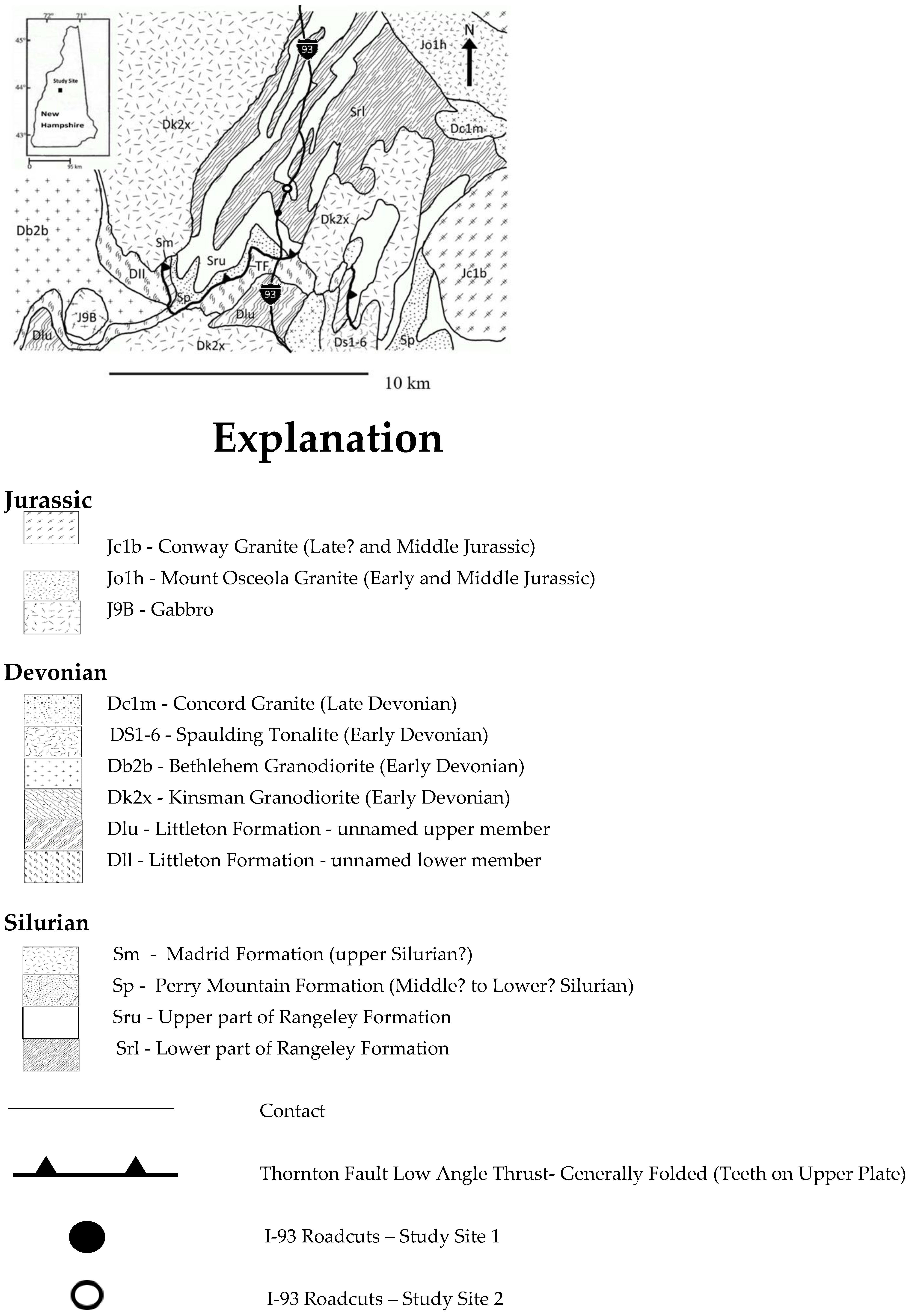
2. Geologic and Tectonic History of the Southwestern White Mountain Region

The bedrock geology of the study site and Hubbard Brook valley has been mapped (sheet 1) at a scale of 1:12,000 [16] and at a scale of 1:10,000 [17]. The study site is also included in earlier bedrock maps [18,19] and at a scale of 1:250,000 [20]. The bedrock underlying the study site (Figure 1) consists of metamorphic rocks intruded by igneous rocks and belongs to the Central Maine Trough [20]. The metamorphic rocks of the Rangeley and Perry formations were deposited as sandy, clay-rich marine sediments [21] on a continental shelf, rise, and abyssal plain of the Rheic Ocean [22] over a time spanning the Silurian (approximately 443–428 Ma). These sediments were then buried and multiply folded by at least two deformation episodes [17] in the Acadian orogeny (early Devonian, 410–390 Ma), as the Rheic Ocean closed and Avalon collided with eastern North America. At this time, the rocks were metamorphosed to the lower sillimanite grade (approximately 600 °C and 4 kb pressure, equivalent to a burial depth of approximately 15 km), which resulted in local melting (migmatization). At approximately 410 Ma, these rocks were at or near the conditions of maximum pressure and temperature and were intruded locally by the southern portion of a large pluton of the Kinsman granodiorite of the New Hampshire plutonic series. The Kinsman granodiorite underlies most of the western half of the Hubbard Brook Valley immediately to the west of the study site [16] see Figure 1. Near the bottom of Figure 1 is a low angle thrust called the Thornton Fault on [20]. This fault thrusts older Silurian rocks over younger Devonian rocks. The fault is cutoff by and therefore must be older than the intrusion of the Kinsman Granodiorite, but younger than the Littleton Formation. This fault extends below the study site and below the Rangeley Formation at the study site. This fault may have formed during Tectonic Event 1 in Table 1 and Table 2. During the late Devonian (370–365 Ma) the metamorphic rocks and the Kinsman intrusion were multiply intruded by small tabular dikes and small discordant bodies of Concord granite, also of the New Hampshire plutonic series. The Concord granite is shown on the map at a scale of 1:200 [16] and in well logs [23], but is not shown in Figure 1 which is modified from the map of [20] (scale of 1:500,000).
The Alleghenian orogeny (325–260 Ma) created the Appalachian Mountains principally by collision with North Africa. While it may not have resulted in large scale deformations at the study site, it was strong enough to create or reactivate fractures.
From early to late Jurassic (194 to 155 Ma) the are immediately to the east and north of the study site was a region of extensive granitic intrusion expressed by the huge batholiths and ring dikes of the White Mountain plutonic/volcanic series [24]. During that time or possibly later (130 to 100 Ma), the metamorphic and igneous intrusive rocks at the study site were intruded by tabular diabase dikes, emplaced as part of continental rifting associated with the opening of the present Atlantic Ocean basin.
From the time of the Acadian Orogeny to the present, erosion and uplift have brought the bedrock from a depth of approximately 15 km to at or near the Earth’s surface. The last episode of deformation was the loading and unloading of the bedrock by the advance and retreat of multiple glacial ice sheets over this region in the past 100,000 years [25]. Reconstructions of the thickness of the Laurentide ice sheet yield a glacial ice loading and unloading of three kilometers for New England [26].
Based upon the orientation of glacial striations, the last Wisconsin Ice sheet moved over the study site from WNW to the ESE [16]. At the last glacial maximum 14,000 years ago, the minimum thickness of the ice at the study site was approximately 1.6 km [27]. The glaciers swept away the thick loess, soils and vegetation that previously covered the bedrock. In some places, the advancing glacial ice plucked automobile-sized blocks from the leeward side of the ridges and small hills in the Hubbard Brook valley. Throughout the valley, glacial ice and water carved and polished the top of the bedrock to a smooth, undulating surface. Finally, as the ice sheet melted in place, the rock debris within the glacier, worked by rivers and streams on top of, within, and beneath the melting ice, was deposited as discontinuous layers on top of the bedrock surface with thickness increasing from 0 at and near the ridge crests and stream beds to as much as 50 m in the lower part of the valley [27]. Because of the glaciation-related erosion, the present-day rock condition of bedrock exposures is extremely fresh, which makes our study of brittle structures much easier than if it were weathered rock.
The geology and faults studied in this report are exposed in roadcuts along Interstate 93 (Figure 2) which were mapped at a scale of 1:200 by [16] sheet 2. All naturally occurring fractures greater than one meter in scale are shown on the map. Fracture orientation, trace length, aperture, surface roughness, and interconnectedness were measured and analyzed [16,28]. The compositional variability in the schist persists to the millimeter scale. The schist has a well-defined foliation, which has been refolded at least twice, and the foliation can be highly variable at length scales less than a meter. At larger scales, the foliation strikes from 25 to 45 degrees east and dips steeply to the southeast, consistent with the regional tectonic fabric.
The granitic rocks intrude the schist in the form of small tabular dikes and large anastomosing fingers ranging from 1000′s of meters to the meter scale. The intrusion was prolific, and granitic rocks account for approximately 50% of the rock area mapped in the road cuts, Figure 2 [16] sheet 2. and in the 40 boreholes (totaling 4.6 km of wellbore) drilled in the Mirror Lake watershed, located at the eastern end of the Hubbard Brook valley [23]. Changes in lithology between granite and schist occurs every 5–9 m in the roadcuts [16] and the boreholes [23].
Bedrock fractures in the roadcuts, natural outcrops and the bedrock wells include joints (formed as Mode 1 fractures), faults (formed as Mode 2 fractures), and reactivated faults and joints. Fractures formed prior to the maximum burial and temperature (410–390 Ma) would have been destroyed by metamorphic recrystallization. We therefore assume that all the fractures that we observe in outcrop were formed after the peak metamorphic event at approximately 390 Ma. It is not possible to determine the age of fracture formation or reactivation using relative or radiometric dating. The brittle tectonic activity since 390 Ma could result from events during the Alleghenian orogeny (Permian, 299 to 251 Ma) and to younger tectonic events, such as the extension related to the opening of the northern Atlantic ocean approximately 200–175 Ma or to the glaciation-deglaciation cycles of the Quaternary (2.6 Ma to present) [27]. Little evidence for the age of brittle events can be obtained from stratigraphy or rock dating, although thin (~1 m) NE-SW striking diabase dikes occur in the study site during the early Jurassic 200–146 Ma may be a brittle episode related to the opening of the Atlantic Ocean. Large numbers of fracture surfaces display syntectonic mineral infill or fiber growth. Because syntectonic minerals like quartz could not develop during the brittle events at very shallow depth, such mineralization indicates that most of the brittle tectonic activity that produced the fault slips took place at depths up to 15 km., and hence is related to tectonic episodes that predate the glaciation-deglaciation events

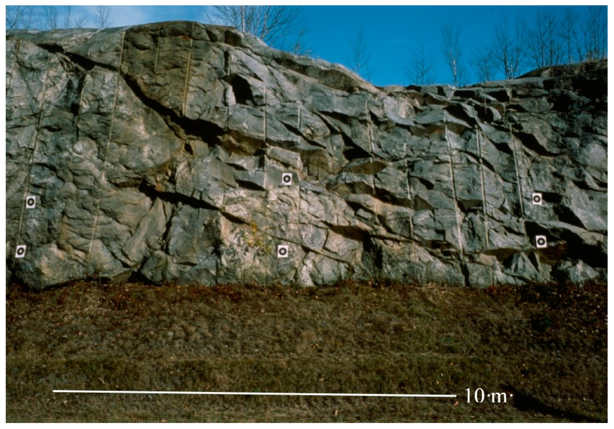
3. Data Collection and Stress Inversion Method of Analysis
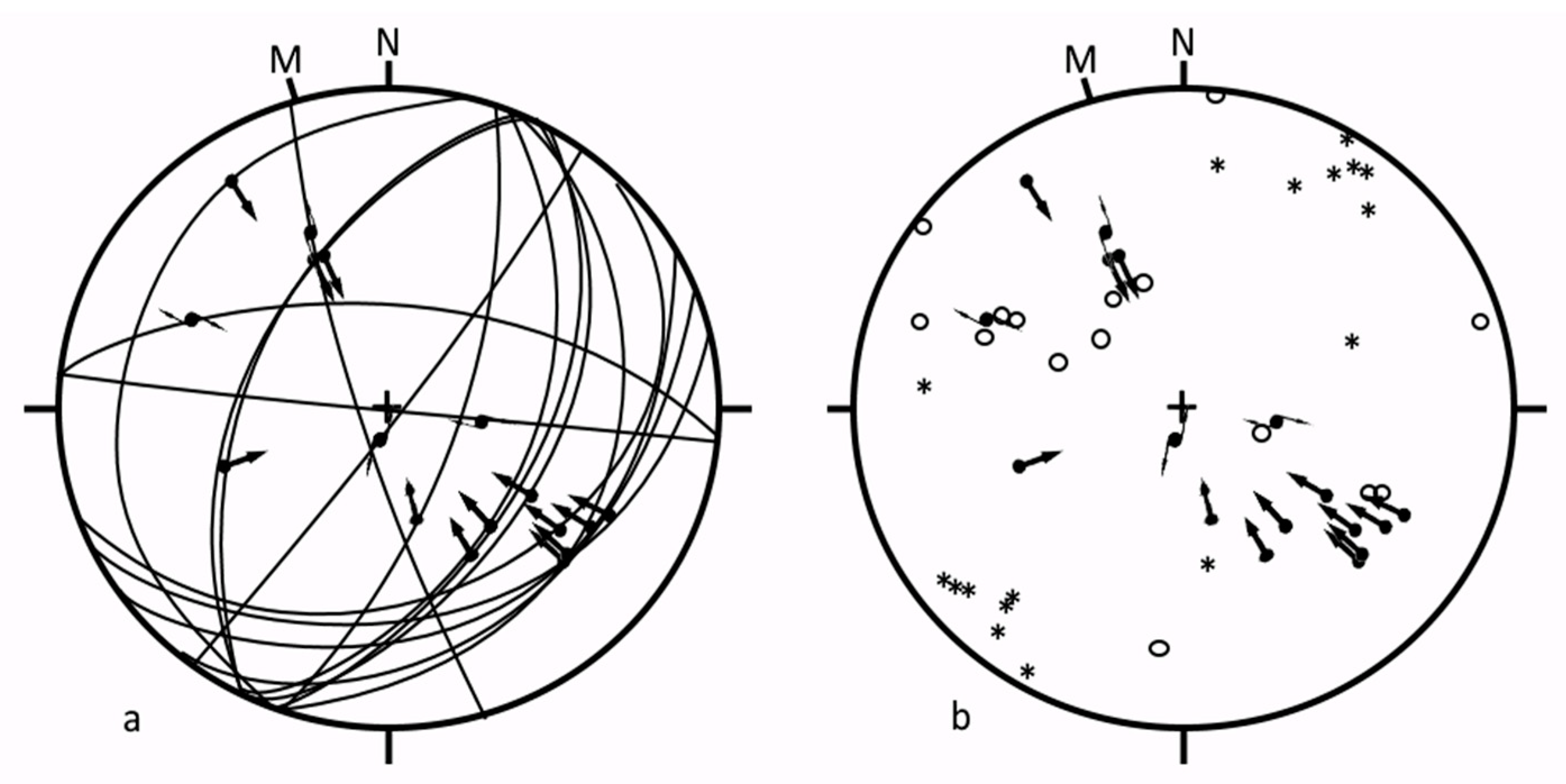
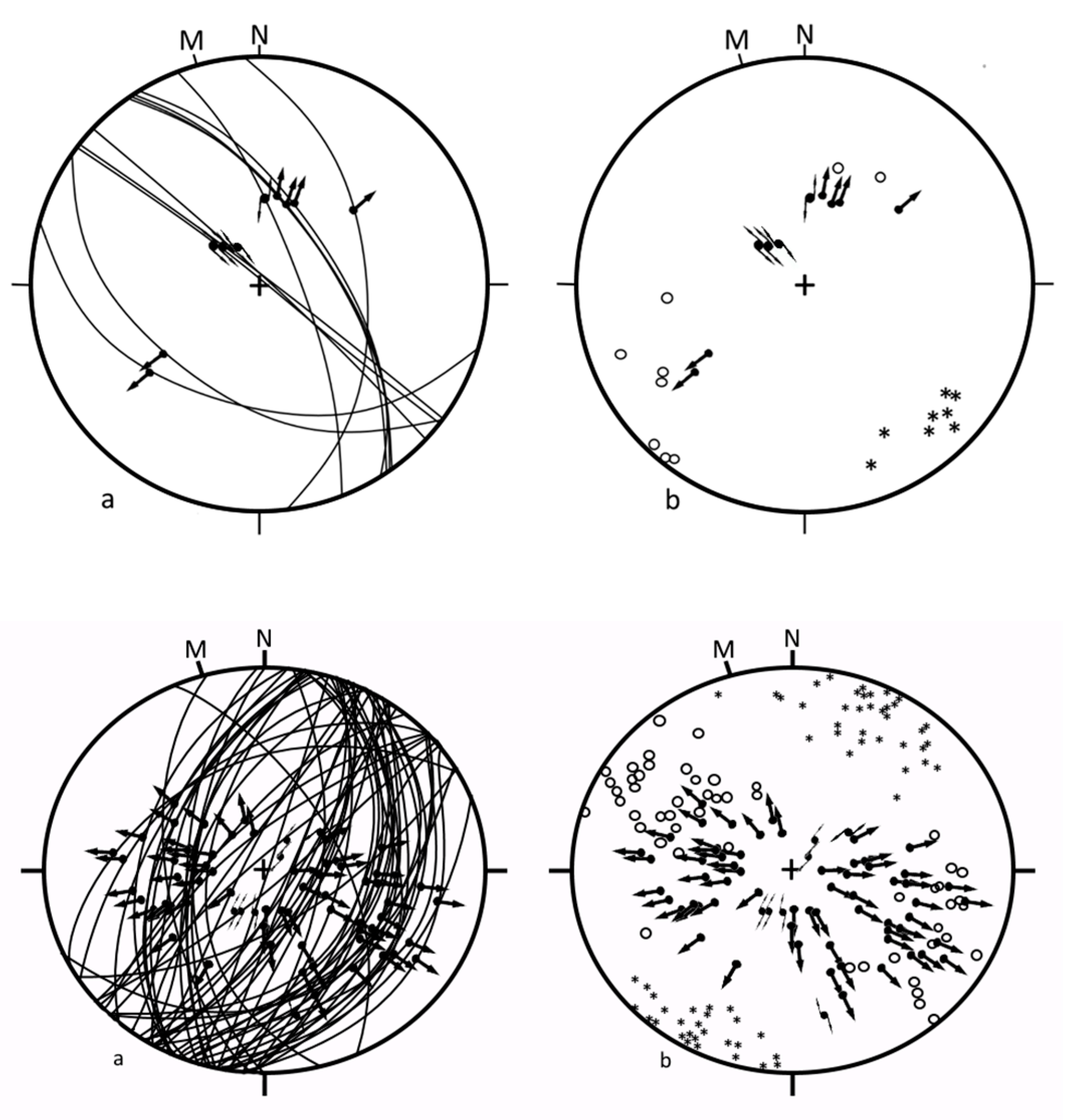
Two hundred and eight fault-slip data were collected at roadcuts in bedrock at two locations on Interstate-93 in Woodstock, New Hampshire as shown in Figure 1. The first location includes four sub-parallel vertical roadcut faces approximately 40 m apart, whose bedrock geology and fractures had been previously mapped [16]. The second location is a roadcut on the east side of the northbound lane of I-93, 1.3 km north of the first location. Figure 2 is a photograph of a section of a portion of roadcut at location 1 showing NE striking, SE dipping fractures in the Concord granite 370–365 Ma.
Faults were easily identifiable in the roadcuts, most of them bearing slickensides resulting from slip-parallel quartz growth. Numerous faults show minor (~1–2 mm) but clearly observable offsets of cleavage, schist-granite contacts, quartz-pegmatite veins, and along contacts of the diabase dikes and the schist and granite. Evidence of slip-parallel quartz growth was common. The strike and dip of the fault plane, the rake of the slickenside lineations, and the sense of relative offset were measured for each observable fault. The faults were numbered. All types of fault slips were found: dip-slip, strike-slip and oblique slip, with normal, reverse, right-lateral and left-lateral components of motion. This variety of fault slips indicates polyphase brittle tectonism, which was confirmed by differences in mineral fillings. The inferred tectonic regime/relative chronology (by number) and level of certainty, the roadcut location, and the fracture number on [16], were all noted. All the information recorded is listed in Appendix A Table A1.
Particular attention was paid to determination of the sense of motion on each fault. A variety of criteria were used, including: (1) offset of granite-schist and other metamorphic boundaries, (2) mineral growth along the slip direction, (3) presence of rough and polished facets along the fault surface, (4) asymmetrical striation markers, (5) striation-related micro-veins, (6) offsets of older fractures or veins, (7) presence of small Riedel’s shear fractures, mainly R in type. Where possible, these criteria were cross-checked. As a result, three levels of certainty were considered concerning the senses of motion (see Appendix A, Table A1). The letter C refers to a slip sense that could be determined with certainty in the field, based on one or several unambiguous criteria. The letter P indicates that the slip sense is considered probable, which means that despite good observation some ambiguity could not be removed. The letter S refers to a poorly recorded sense of motion, in the absence of reliable criterion or with conflicting criteria. In that case an inferred “supposed” sense of motion was attributed, based on both the low-quality criterion (if any) and the behavior of the neighboring faults with well-recorded sense of motion and similar dip direction, attitude, and slip orientation.
Many faults were associated in conjugate or Riedel’s type patterns with particular symmetries. Fault subsets were defined based on common geometry in terms of fault attitude, slip orientation and sense, fault dip direction, relation to other faults, and mechanical consistency. The relation between conjugate fault systems and stress has been highlighted by Daubrée’s experiments [29] and Anderson’s analysis [30]. In addition, Riedel’s shears [11] often explain the relationships between faults at different scales.
Most fault slip data in the outcrops studied could not be interpreted in simple geometrical terms, because they resulted from reactivation of earlier faults or mechanical discontinuities (older faults, joints, veins, cleavage, contacts between rock types, etc.). Such inherited faults may have various attitudes oblique to all stress axes, contrary to the “newly formed” faults discussed above, which generally contain one principal stress axis and form symmetrical systems. For this reason, we undertook systematic inversion of the fault slip data to reconstruct the stress regimes. Such inversions are based on consideration of the stress-slip relationships proposed by [31,32], which were used by [12], who first addressed the inverse problem in their pioneering work. Later studies demonstrated that the basic assumptions underlying the method were acceptable in the first approximation and well accounted for actual slip distribution (e.g. [2,3]), and numerical modeling experiments showed that deviations from the model are significant but remain statistically minor with regard to other sources of uncertainty [33].
The direct inversion method’ used here is based on a least-square minimization, with a criterion called υ (upsilon) that depends on both the angle between the calculated shear and the actual slip, and the shear stress amplitude relative to maximum shear stress. For details, the reader is referred to the paper that describes this method [4]. We also use a robust refining process that was not described in the original formulation of the method but is presented in the use of another method especially designed for the stress inversion of earthquake focal mechanisms [13]. This additional process was facilitated by the negligible runtime of the inversion method, which involves analytical means instead of numerical search. A crucial parameter is the minimum fit level required for defining acceptable data. We use a scale from −100% (total misfit) to 100% (perfect fit). The lowest bound involves maximum shear stress acting in the direction opposite to slip. At the highest bound, the shear stress is also maximum but acts in the same direction and sense as the slip. A zero value indicates that slip occurs with shear stress perpendicular to slip, as the limit between consistent and inconsistent senses of motion. Note that this minimum fit level is linearly related to the RUP % estimator defined by [4], the values −100% and +100% corresponding to the values 200% and zero (respectively) in the RUP estimator and differs from the ω estimator defined by [13].
To determine a stress regime, υ is minimized as a function of the four unknowns that describe a reduced stress tensor: the orientations of the three principal stress axes and the ratio Φ = (σ2 − σ3)/(σ1 − σ3). One obtains the smallest slip-shear angles and the largest possible shear stresses that can simultaneously exist for all the data taken together.
The real data dispersion, which depends on complex geological factors, is larger than the angular uncertainty of about 5° in our field data collection. To determine whether a stress inversion is significant or not, we use an iterative refining process that involves successive inversions with a progressively increasing demand for good individual fits. This process allows determination of the level of data rejection consistent with the data accuracy.

4. Results

Based on consideration of relationships between fault slips (crosscutting relationship, reactivation of fault surface, etc.), spatial association between faults (e.g., conjugate patterns) and syntectonic mineral growth (e.g., quartz fibers), and taking into additional account the mechanical consistency within each subset of fault slips, it was possible to separate nine data subsets (regimes), as listed in Table 1 below.
The number of Regimes is large (9). High confidence can be placed in the definition of the regimes themselves, their sequential order, and especially the directions of compression and extension of the inferred stress tensor. A second step involves grouping the Regimes into tectonic Events where the known regional tectonics coincides with the direction of the principal stresses and the time sequence of known regional tectonic events. The grouping into Events is shown in Table 2 and discussed below.
Each Regime is depicted on a lower hemisphere equal area projection below showing the great circles of each of the fault planes determined. Arrows indicate the slip on the fault planes. A separate companion plot displays the same arrows and the poles to the fault planes (open circles) and the trend and plunge of the intermediate stress (σ2). Arrows pointing toward the center of the projection indicate compression. Arrows pointing to the perimeter of the projection indicate extension. Solid circles with two arrows pointing in opposite directions indicate the sense of strike-slip movement. Those with no arrowheads have an indeterminate sense of movement.

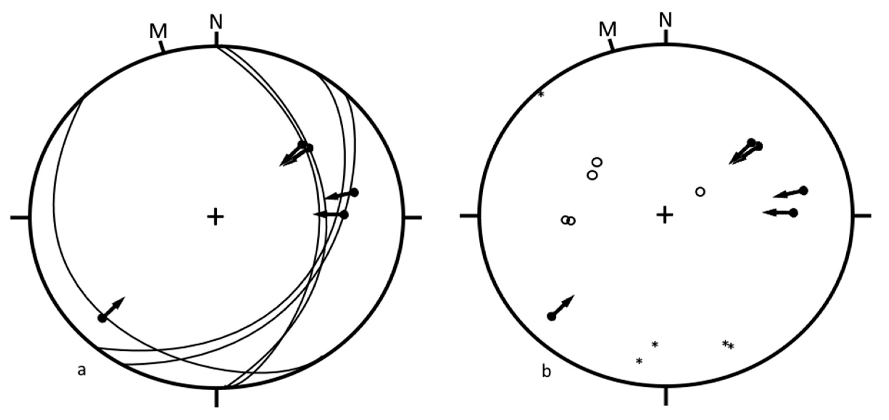
4.1. Event 1—Regime 1

This regime is characterized by reverse faults compatible with a NW-SE compression (Figure 3). The frequent presence of quartz veins and along-slip quartz growth indicate that slip probably occurred close to the ductile-brittle transition. The relatively deep and hot character of this tectonic deformation suggests that this event is the oldest event.
The stress inversion of fault slip data for this data subset shows that for a reasonable threshold, MIFL = 40%, only 2 of the 19 fault slip data are considered unacceptable. Similar solutions were obtained for minimum individual fit levels of 20% (no data being eliminated) or 40% (4 data eliminated). The stress regime determined is thus stable.
The calculated stress regime indicates a nearly horizontal compression that trends 133° N. The stress axes σ2 and σ3 are oblique, with plunges of 45°, in agreement with the low value, 0.13, for the ratio Φ = (σ2 − σ3)/(σ1 − σ3). This low Φ reveals σ2 and σ3 are closer in magnitude than either is to σ1. The solution cannot be considered very accurate because the number of acceptable fault planes inversions is small (17). The direction of compression is constrained within ±10 degrees, but the values of Φ and the attitudes of stress axes σ2 and σ3 may vary widely as a function of data removal within this set. In summary: the oldest brittle tectonic episode that we can recognize corresponds to a NW-SE compression that reactivated deep fractures in reverse faulting.

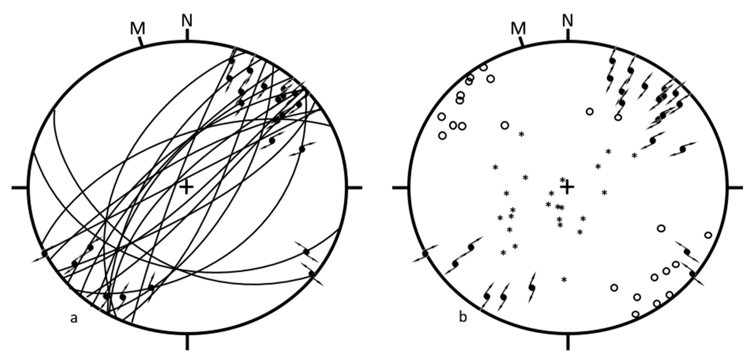
4.2. Event 2—Regimes 2 and 3

In contrast to Regime 1, both Regimes 2 and 3 are dominated by normal fault extension (Figure 4). Most are dip-slip, which suggests a low level of structural inheritance and reactivation of earlier structures. Most fault surfaces are planar with relatively steep dips, which suggests that they developed at shallower crustal levels than the reverse faults of Regime 1. However, the gentle dips of some of the normal faults suggests the reverse faults of Regime 1 have been reactivated as normal slips. Note that the dominate trend of normal faults in Regime 3 are the same as for the reverse faults of Regime 1 (e.g., the fault poles are similar). Syntectonic quartz is common on the surfaces of these inherited normal faults, with the quartz probably inherited from Regime 1.
The two subsets of faults strike at right angles. The normal faults of Regime 2 strike NW-SE. and the normal faults of Regime 3 strike NE-SW. Regime 2 faults indicate NE-SW extension whereas Regime 3 faults indicate NW-SE extension.
The stress inversion of fault slip data for Regime 2 is stable (2 faults rejected at MIFL = 55%, no faults rejected at 20%, and only 4 of the 20 faults rejected at MIFL = 80%), but is only loosely constrained because of the limited number of data (18 acceptable faults). As with Regime 1, the numerical results are good, but the solution is highly dependent on the grouping of data. For example, removing the two nearly vertical faults results in a significantly different solution. The stress regime at MIFL = 55% indicates a 33° ± 10 degrees trending extension with oblique σ1, σ2 and σ3 axes. The σ3 axis plunges 33° NE, which is not surprising in light of the presence of nearly vertical faults with the downthrown side to the northeast. The Φ ratio of 0.46 indicates triaxial stress.
In contrast, the large number of fault slip data in Regime 3 provides a highly constrained stress tensor solution. The solution is stable (13 of 75 faults rejected at MIFL = 40%, 4 at 20% and 20 at 55%). The stress orientations and Φ are similar regardless of the MIFL, which indicates that the stress tensor is well constrained. On the other hand, the slip vectors have a large scatter (Figure 4). The number and geometrical variety of the data are more important than the average of parameter estimates and their standard deviations. Removal of fault slip data does not change the inversion results within the range of uncertainties, which confirms that geometrical constraints on the stress tensor exerted by the variety in fault slip attitudes is more important to a good interpretation. At MIFL = 40% the σ1 axis is nearly vertical and indicates a 110° azimuth of extension (the σ3 axis plunges only 3° to the west). The direction of extension is constrained within ±5 degrees. A Φ ratio of 0.49 indicates typical triaxial stress.
No clear chronological difference could be established between Regimes 2 and 3. The perpendicularity in fault trends and corresponding directions of extensions strongly suggest that these two regimes are linked through a permutation (relative magnitude switch) between the intermediate and minimum principal stresses, σ2 and σ3. These two regimes thus probably belong to a single major extensional event which we identify as Event 2. Because Regime 3 is represented by a much larger number of brittle structures than Regime 2, the dominating direction of extension is inferred to be WNW-ESE (azimuth 110°). A tensor inversion with Regimes 2–3 taken together shows that the influence of the fault slip data from Regime 3 prevails, and the combined tensor solution resembles that of Regime 3. For a MIFL = 30% the Φ ratio is lower (0.35) but the direction of extension is similar (115°). The stability of the solution is much less, which suggests the distinction between Regimes 2 and 3 is in fact significant in terms of stress states, even though both are produced by the same tectonic event. Brittle tectonic analyses have revealed significant changes in stress regimes within a single tectonic episode [4,5,6,13,15]. The duality of stress regimes (2 and 3) may simply result from a permutation between the σ2 and σ3 axes, a common phenomenon in fault tectonics.
Although there remains some indication of ductile-brittle transition for some faults with abundant quartz coating and slip-parallel quartz growth, most Event 2 faults are typically brittle, as shown by both the fault surface characteristics and their steep dips. Relative chronologies with respect to other events show that Regimes 2 (certainly) and 3 (probably) post-dated the Regime 1. Our data thus suggest that the extension of Regimes 2–3 post-dated the compression of Regime 1 and suggests that Regimes 1–3 reflect the oldest two faulting events well represented at the site.

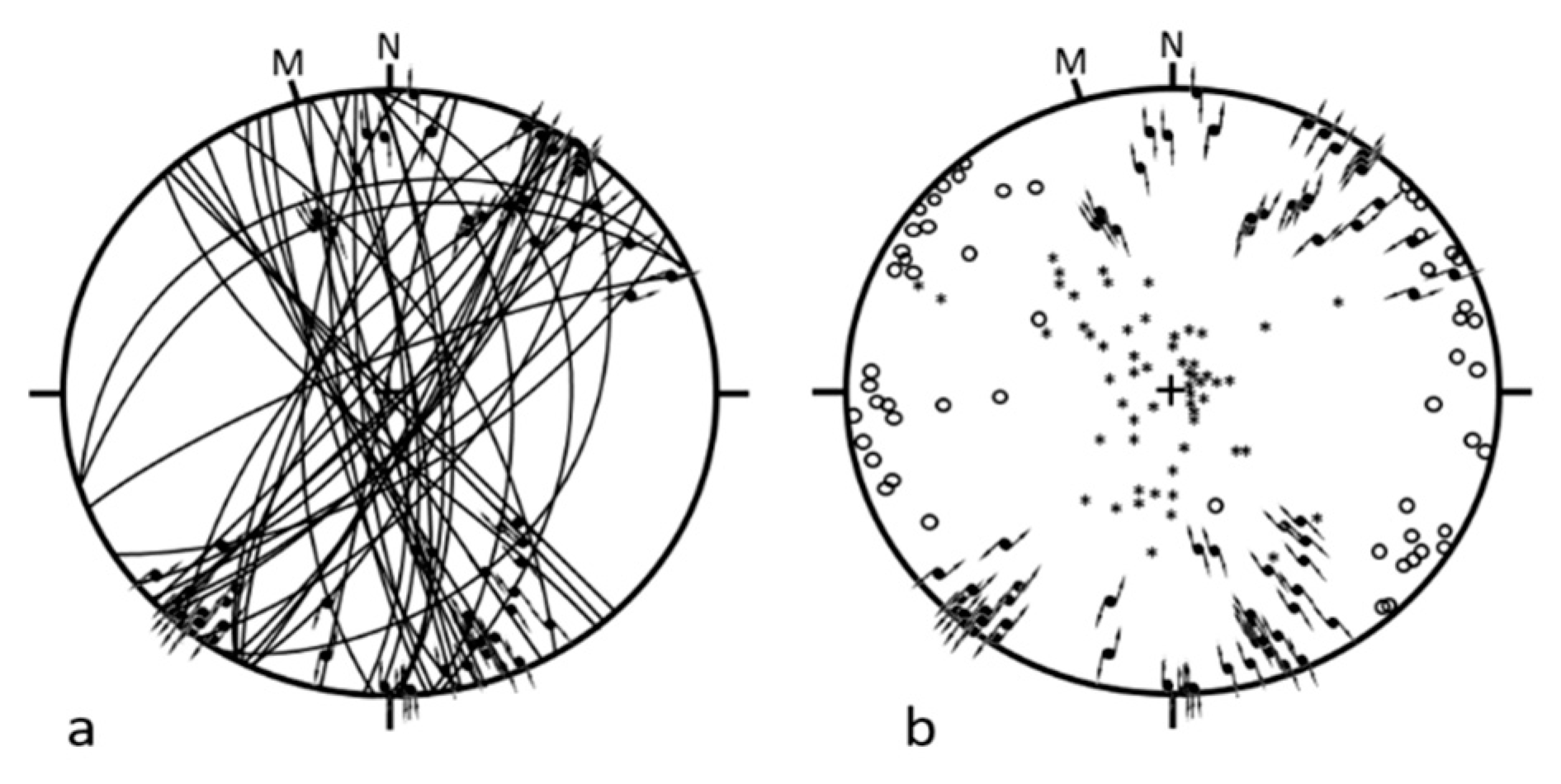
4.3. Event 3—Regime 4

Regime 4 is poorly represented. It is characterized by only a few reverse faults that are compatible with a NE-SW compression. The stress inversion provided stable results, which has little meaning because of the very low number of faults (5). The tensor solution is very loosely constrained. Had more fault slips been identified, the result would have been subject to significant variations. For a MIFL = 45% one of the five faults is considered unacceptable, and the calculated stress regime indicates a 59° compression direction with a nearly vertical σ3 axis and a Φ ratio of 0.44. The direction of compression may however vary within ±20°.
The reverse faults shown in Figure 5 are younger than those of Regime 1, but there is little indication of their age. Two display the same attitude, but different oblique slip vectors from the reverse faults of Regime 1 from which they are inherited.

4.4. Event 3—Regime 5

Regime 5 (Figure 6) is better represented than Regime 4. The stress tensor inversion indicates strike-slip faulting consistent with a nearly E-W compression and N-S extension. These strike-slip faults clearly postdate the reverse faults of Regime 1. The stress tensor inversion is stable (1 of 24 faults rejected at MIFL = 55%, none rejected at 25%, and 7 rejected at MIFL = 70%). Another indication of inversion stability is that the removal of dextral fault slips does not significantly modify the inversion results.
The stress regime calculated at the MIFL = 55% level is characterized by a nearly horizontal σ3 axis that trends 0° and a gently plunging σ1 axis whose azimuth trends 83°. The direction of extension is not more tightly constrained than ±10 degrees because only 2 left-lateral faults were measured. A typical triaxial stress is indicated by the Φ ratio of 0.50.
Contrary to the typical, most strike-slip faults of Regime 5 are far from vertical. Many of the right-lateral faults dip towards the NW or SE, which suggests that they were inherited from the normal fault planes of Regime 3. Two left-lateral faults have gentle SW dips, which suggests that they were inherited from normal fault planes of Regime 2.
Although the faults of Regime 4 are reverse and the faults of Regime 5 are strike-slip, the directions of compression are similar considering the large angular uncertainty in the trend of compression of Regime 4. For this reason, we combine Regimes 4 and 5 within a single Event 3 that is dominated by a roughly E-W compression and can generate both reverse and the strike-slip faulting. The stress tensor for this combination resembles that for Regime 5 because of the larger number of faults in Regime 5. Unlike the combination of Regimes 2 and 3, the combination of Regimes 4 and 5 shows good stability (1 of 30 faults eliminated for MIFL = 20%, 9 for 55%). But the rejected faults are 2 of the 5 reverse faults of Regime 4, and the individual misfits of the three remaining Regime 4 reverse faults are large. The simplest solution suggests mixing Regimes 4 and 5 are indeed distinct.
For a reasonable fit level of 35% (2 faults rejected), the Φ ratio is 0.43, indicating triaxial stress despite the mixture of strike-slip and reverse faults. The stress regime is characterized by a gently plunging σ3 axis with a trend azimuth of 351° and a nearly horizontal σ1 axis with a trend of 83°. The data indicate stress regimes 4 and 5 belong to a single event dominated by WNW-ESE compression and that a permutation between σ2 and σ3 changes the faulting from reverse to strike slip.

4.5. Event 4—Regimes 6, 7 and 8

The strike-slip faults of Regimes 6–7 are shown and analyzed together (Figure 7). These regimes are dominated by strike-slip faulting. Sixty-nine faults are observed, the largest ones forming typical strike-slip zones composed of two walls on either side of a 1–3 m wide deformed zone with numerous smaller faults, fractures, rotated blocks, and gouge. The strike-slip faults strike approximately NNW-SSE for right-lateral faults, and NNE- SSW for left-lateral ones, indicating N-S compression.
The stress tensor solution is tightly constrained by the large number of the faults and the variety of their orientations (17 faults rejected at MIFL = 45%, 5 at 20%, and 23 at 55%). The stress orientations remain extremely stable as the MIFL increases. In addition, removal of fault slip data does not significantly affect the inversion. The geometrical constraints exerted by the variety in fault slip attitudes are strong. Because a significant overlap in stress trends is present between right-lateral and left-lateral faults, several data displayed incompatible senses of motion. This explains why faults were eliminated even for low levels of MIFL. Separation into two Regimes, 6 and 7, solved this problem and reduced the number of inconsistent senses to zero for each of the stress tensors, but was not retained because no independent qualitative evidence supported a separation of these Regimes.
The stress regime calculated at MIFL = 45% is characterized by gently plunging σ1 and σ3 axes (plunges of 14° and 17° degrees respectively), with a nearly N-S trending, azimuth 188°, compression. This direction of compression is constrained within less than ± 5°. The Φ ratio of 0.45 indicates typical triaxial stress.
Relative chronology data provides good evidence that this major strike-slip event postdated the normal faults of Event 3. Although some strike-slip faults of Regime 6 and 7 have relatively gentle dips suggesting that they were inherited from earlier regimes of reverse and normal faults, most of these strike-slip faults are vertical or steeply dipping, cutting through all pre-existing structures rather than reactivating them. It is likely that several NE-SW trending faults result from right-lateral reactivation of the left-lateral faults of Regime 5, but observation is speculative because of the right-lateral friction that generally destroyed the criteria supporting the evidence of an earlier left-lateral motion.
Regime 8 is represented by only a few dip-slip reverse faults (Figure 8). The relative chronology data indicate that this regime occurred before the Regimes 6 and 7. As with Regime 4, the stress inversion provides very stable solutions, but this stability is not significant because the number of faults is so small. The tensor solution is in fact poorly constrained. For MIFL = 50%, all data are acceptable, and the calculated stress regime indicates an azimuth 330° compression with a nearly horizontal σ1 axis, a steeply plunging σ3 axis and a Φ ratio of 0.23. The direction of compression is constrained within ±20°.
Because the direction of compression suggested by this pattern of reverse faults is not far from N–S (with an azimuth of compression approximately 160), they may be related to regimes 6–7 through a relative magnitude shift between the intermediate and minimum stress axes. If Regime 8 is added to 6 and 7 the inversion rejects all 4 faults in Regime 8. As in the case of Regimes 2–5, this suggests a common tectonic event involving a stress permutation between σ2 axis and σ3 axes. There is no evidence that Regime 8 resulted from a separate tectonic event.
Event 4 comprising Regimes 6–8 was certainly more recent than the reverse and normal faults of the ductile-brittle transition (compression of Regime 1, and the extension of Regime 2). The contacts of the diabase dikes of Jurassic age are reactivated as strike-slip faults of Regimes 6 and 7 indicating that the faulting and diabase dike intrusion in these regimes occurred 200–146 Ma or later. The NW-SE extension is compatible with the regional extension (based on local NE-SW diabase dike trends, [24]) affecting the study area during the initial opening of the north Atlantic Ocean 200–175 Ma [34], Figure 5.

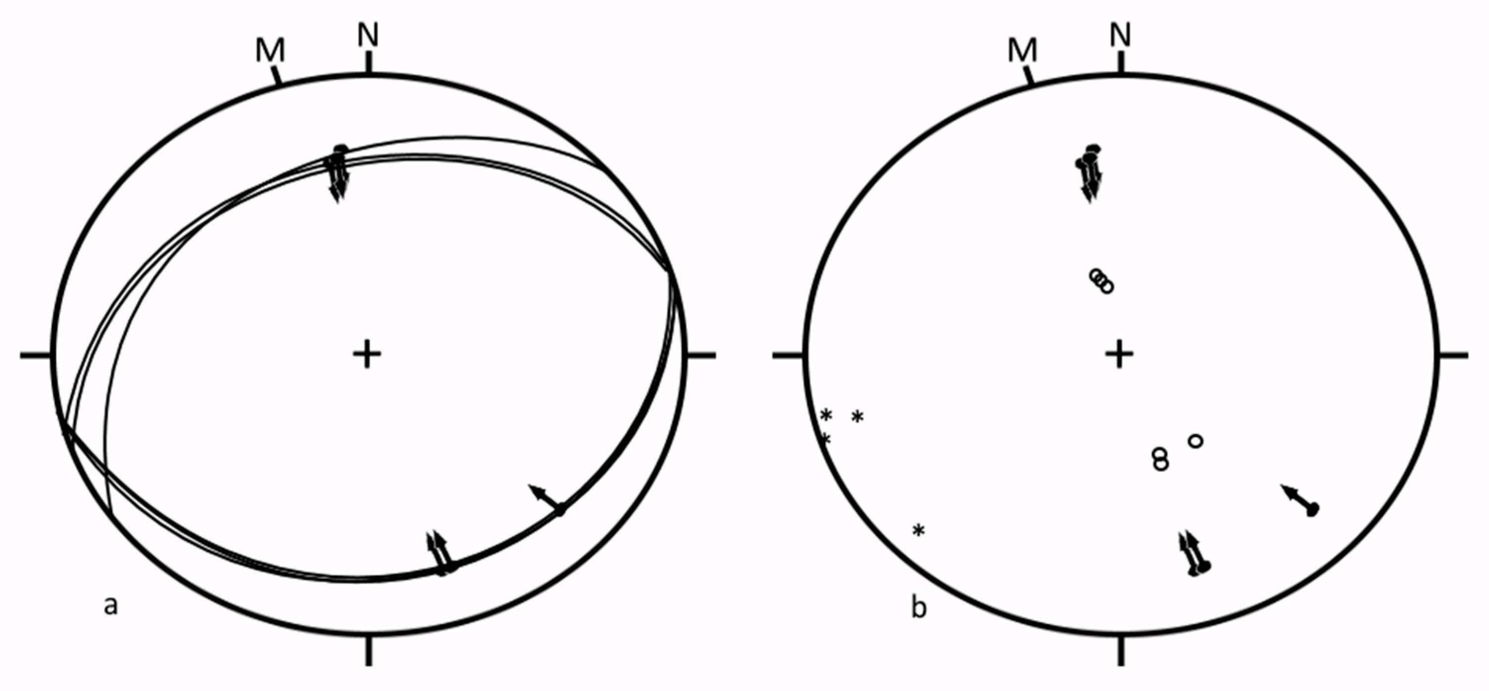
4.6. Event 5—Regime 9

Regime 9 (Figure 9) corresponds to three strike-slip faults, which trend NW-SE (left-lateral) and WNW-ESE (right-lateral), and hence indicate a roughly NW-SE compression which we label as Event 5. This event is the most recent at the study site. Designation of Regime 9 and calculation of the stress tensor by three fault slips results in a high level of uncertainty.

5. Interpretation

We relate the relative stress tensor in our Events (Table 2) to known tectonic events summarized above in Section 2.

5.1. Event 1—Acadian Compression

This major event is the oldest episode recorded by fault slip at the study site. It was dominated by NW-SE compression (Regime 1) and took place at depth, near the ductile-brittle transition at the or near the end of the Acadian orogeny (390–375 Ma).

5.2. Event 2—Post Acadian Extension

This major event was responsible for widespread normal faulting at a depth, not far from the ductile-brittle transition. Its faults developed under a pure brittle regime at shallower depths, and the faulting was later (375–325 Ma)-than the faults in Event 1. The major NW-SE extension that occurred in this Event parallels the major NW-SE compression of Event 1. This suggests that the extension in Event 2 resulted from the exhumation of metamorphic basement that followed the major compressional phase of Event 1.

5.3. Event 3—Late Alleghenian Compression

The reverse and strike slip faulting of Regimes 4 and 5 are not numerous enough to tightly constrain the corresponding paleo-stresses, and these two Regimes are poorly located in time. They are represented by pure brittle features, and certainly postdate the brittle-ductile deformation, but may not predate Event 4. We tentatively relate these two regimes to the late tectonic evolution of the Alleghenian orogeny (325–260 Ma).

5.4. Event 4—Atlantic Extensional Opening (?)

The strike-slip faulting of Regimes 6 and 7 and the reverse faulting or Regime 8 indicate N–S compression and E-W extension. The presence of a strike-slip fault zone 1–3 m wide suggests that the offsets are relatively large (10–100′s of meters) [35,36,37]. The contacts of the diabase dikes of Jurassic age are reactivated by the strike-slip faults of Regimes 6–7 indicating that the faulting and diabase dike intrusion in these regimes occurred 200–146 Ma or later. The NW-SE extension is compatible with the regional extension (based on local NE-SW diabase dike trends, [24]) affecting the study area during the initial opening of the Atlantic Ocean 200–175 Ma [34], Figure 5.

5.5. Event 5—Recent or Present

This Regime is represented by only a few strike-slip faults with minor offsets. The direction of compression (NW-SE) is consistent with the present state of stress in this region based on earthquake focal mechanisms [38]. We did not observe sheeting joints (sub-horizontal fractures) that can form in response to the unloading of glacial ice [39] over the past 100,000 years.

6. Discussion

This paper illustrates a method to identify distinct regional tectonic events and put them in relative chronological order from fault slip data collected on a few local roadcuts. The data was collected in this case over a period of 10 days. The volume of fault orientation and slip data is relatively small compared to regional field mapping of large scale structures field studies, but by explicitly considering the stress tensors that could have produced the observations, the fault data can be sorted and grouped into Regimes that yield compatible stress tensors that can be further grouped into distinct tectonic Events. In the southwest White Mountain region, the Events identified correspond to known tectonic events based on large scale structures over the last ~400 Ma. The orientation and relative magnitudes of principal stresses producing major regional tectonic deformations can be obtained relatively quickly from a study at one locality.
The conditions for this study were close to ideal because the roadcuts exposed unaltered rocks recently exhumed by the last glaciation. The direct inversion method could potentially be applied using oriented cores from boreholes where there are no outcrops. This paper illustrates how, if the stress tensor can be constrained, the history of overprinted deformation that could have impacted basin resources can be deduced from features on the surfaces of fractures reactivated by sequential tectonic events.

Author Contributions

C.C.B.: field collection of data 50%, writing of manuscript 90%. J.A.: field collection of data 50%, inversion of data and identification of regimes and events 95%, writing of manuscript 10%. All authors have read and agreed to the published version of the manuscript.

Funding

C.C. Barton was supported by the U.S. Geological Survey as part of his employment. J. Angelier was supported by the Universite Pierre et Marie Curie as part of his employment.

Acknowledgments

The authors wish to acknowledge support from the U.S. Geological Survey. J. Angelier was an early key developer of the Direct Inversion Method of Fault-Slip Analysis for unraveling tectonic history to deduce paleo stress orientations and relative magnitudes from surface structures on the faces rock fractures reactivated by sequential tectonic activity. Readers are directed to his many papers on this subject. He was a pleasure to work with in the field. His field notebooks were magnificent and artistically beautiful. His intelligence, enthusiasm, and good company is missed by those who knew and worked with him. Jacques Angelier died in January 2010. The authors thank Tristan Coffey who drafted the figures and tables. The authors thank C. Page Chamberlain and Gautum Mitra who provided early reviews of this manuscript and two anonymous additional reviewers. The authors also thank Lawrence Cathles who provided a thorough edit for this volume

Conflicts of Interest

The authors declare no conflict of interest.

Data Availability

The data collected for each fault listed in tabular form in Appendix A is also available at: http://www.hubbardbrook.org/data/dataset_search.php.

Appendix A. List of Data Collected in This Study

  • Explanation to Columns in Table A1
  • Column A–Fault Reference Number
  • Column B–Fault Strike (azimuth)
  • Column C–Fault Dip and Direction
  • Column D–Rake of Slip Striations
  • Column E–Regime Number/Relative Chronology (1 = oldest, 9 = youngest)
    • Certainty (C = certain, P = probable, S = inferred)
  • Column F–Fault Location on Interstate 93:
    • SBLW = Southbound Lane, West Side of I-93, [10] sheet 2
    • SBLE = Southbound Lane, East Side of I-93, [10] sheet 2.
    • NBLW = Northbound Lane, East Side of I-93, [10] sheet 2
    • NBLE = Northbound Lane, West Side of I-93, [10] sheet 2
  • Column G–Fracture Reference Numbers on [10] sheet 2
  • Column H–Site location (see Figure 1)
Table A1. Fault Data Collected and Analyzed in This Study.
ABCDEFGH
117377W43N6CSBLE11
24140E45N2C 4CSBLE421
33238E62N2C 4CSBLE421
49564N40W1C 1CSBLE42A1
516383W40N6CSBLE11A1
616383W40N1CSBLE111
716685W44N6CSBLE11A1
816583W38N6CSBLE11A1
915977W9S7CSBLE191
1015288W20S7CSBLE14B1
1115978W17S7CSBLE14B′1
1215389W34S7CSBLE221
1313789W41S7CSBLE221
1415377W46S7CSBLE221
1516584W46S7CSBLE22′1
1614681W25S7CSBLE211
1714188W43S7CSBLE211
1813988W36S7CSBLE201
1913677W33S7CSBLE201
2015876W24S7CSBLE19′1
21369W31S7CSBLEunmapped1
2215777W23S7CSBLE19′1
23369W31S7CSBLEunmapped1
245548N52W3CSBLEunmapped ou 18A1
256146N47W3CSBLEunmapped ou 18A1
264877N76W3CSBLEunmapped ou 18A1
272963W73S3CSBLE241
282852E68S1CSBLE251
294787S29W7CSBLEunmapped1
304288E3S1C 7CSBLEunmapped1
3117742E61N2C 4CSBLE481
3217844E21S1C 7CSBLE481
3317844E60N2C 4CSBLE481
341848E51S3CSBLE491
352677E25N1C 6CSBLE671
362677E79S2C 3CSBLE671
371351E37S3CSBLE98?1
381288W12S7CSBLEunmapped1
3917660E46N6CSBLEunmapped1
404887N7E1C 5CSBLE1071
414887N75E2C 3CSBLE1071
423087E82N3CSBLE1061
434178E17N5CSBLE116A proche1
1844380E15N5CSBLE116A proche1
1822870W23S7CSBLE1161
1834175E74S3CSBLE1161
445487N29W5CSBLE1161
453266E33S5CSBLEunmapped1
463071E81N3CSBLE1231
473071E18N5CSBLE1231
483972E83S3CSBLEunmapped1
495184S72W1C 3CSBLE1301
501820W53N2C 1CSBLE1381
515184S10E1C 5CSBLE1301
521721W53N2C 1CSBLE1381
535083S73W3CSBLE1301
545083S9E5CSBLE1301
557334S63E1CSBLEunmapped1
566741S66E1CSBLE1391
575976N28E5CSBLE1461
586663N28E5CSBLEunmapped1
595776S15W5CSBLE1621
602474E12N1P 5CSBLE1661
612474E30N2P 7CSBLE1661
622474E64S1P 3CSBLE1661
632575E30N2P 6CSBLE1661
644787N22E6CSBLW661
659689S67E1CSBLW491
665786S37E5CSBLW481
671788E73S3CSBLEunmapped1
682556W61S2C 1CSBLW251
692556W62N1C 1CSBLW251
702556W16S2C 5CSBLW251
712554W64N1C 1CSBLW251
727133N82E1C 8CSBLW241
737133N42E2C 6CSBLW241
745232N63E8CSBLW241
757622S58E1C 8CSBLW241
767131N82E2C 8CSBLW241
777821S84E8CSBLW241
787523S88E8CSBLW241
79770E62S3CSBLWunmapped1
801043E76S3CSBLunreferenced1
812971W24N5CNBLW11
823776W29N5CNBLW11
834274W35N5CNBLW11
844872N12E5CNBLW11
8514219W85S4CNBLWunmapped1
866833S64E3CNBLW91
876935S37E3CNBLW 1
884652S63E3CNBLW12-11月1
895247S63E3CNBLW12-11月1
905138S52E3CNBLW121
914642S84E3CNBLW131
924544S83E3CNBLW131
931420E73S3CNBLWnear F291
942225E85S3CNBLWnear F291
952133E74S1CNBLW281
962154E72S1CNBLW281
975833S67E1CNBLWunmapped1
984658S66E3CNBLWunmapped1
994127E77N1CNBLW351
1002950E72N3CNBLW711
1013181E18S5CNBLW731
1026781N6E7CNBLWunmapped1
1033889E9S7CNBLWunmapped1
1042454E64S3CNBLW791
1051530E73S3CNBLW791
1061036E68S3CNBLW791
1072946E87S3CNBLW801
1082948E89S3CNBLW801
1352948E88S1CNBLW801
10911069N11E9CNBLWunmapped1
11013989E19S9CNBLWunmapped1
1112085W12N5CNBLW 1
11216557W60S3CNBLW 1
1136386N1W5CNBLW 1
1142165E76N3CNBLW861
11516083E4S7CNBLW122?1
11616180E14S7CNBLW123?1
11715075E10S7CNBLW123?1
11816684E7S7CNBLW1181
1192583E2N7CNBLWunmapped1
12017776E2S7CNBLWunmapped1
1212651E64N3CNBLWunmapped1
122182E2S7CNBLW130?1
12317086E7S7CNBLW133?1
124482E1N7CNBLW131?1
1251447E79S3CNBLWunmapped1
1264747S33E5CNBLW1351
12717962W80N3CNBLWunmapped1
128167W84N3CNBLW1511
12915677W2S7CNBLWunmapped1
1301269W87S3CNBLW1561
1313377W3S7CNBLW1561
132757W71S3CNBLWunmapped1
1331364W77N3CNBLWunmapped1
134855W72S3CNBLWunmapped1
18515562E80S3CNBLWunmapped1
1862882E77S1C 3CNBLWunmapped1
1872882E4N2C 7CNBLWunmapped1
1363279W79N3CNBLEunmapped1
1373472E74N3CNBLE361
1383485E8S7CNBLElarge fault1
1393666E2N7CNBLElarge fault1
14017475E17N7CNBLEunmapped1
14117683W27N7CNBLE461
14217588E15N7CNBLE461
14317879E2S7CNBLE531
1443039E10N2C 7CNBLE511
1453039E75S1C 3CNBLE511
1463288W6N7CNBLE551
1474186E3S7CNBLE641
1483782W1S7CNBLE641
1491761E83S3CNBLE581
1503573W63S3CNBLEunmapped1
15111484N5E9CNBLE681
1524285E1S7CNBLE701
1535089S7W7CNBLE741
1543582W12S7CNBLE741
1554488E6S7CNBLE741
1564072W11S7CNBLE87-891
1573981W1S7CNBLE87-891
1582985W36N7CNBLE87-891
1591083W14N7CNBLE87-891
1603280E84N3CNBLE911
1612984E28N7CNBLE911
1624672N88E3CNBLE981
1635868S76E1C 3CNBLE1051
1645868S22E2C 7CNBLE1051
1653542E82N3CNBLEunmapped1
1661973E66S1CNBLEunmapped1
1672247E80N3CNBLEunmapped1
1685273S13E7CNBLE1111
1694689N12E7CNBLE130?1
1703682E34N2C 7CNBLE136?1
1713682E 1C 3CNBLE136?1
1722249W64S3CNBLEunmapped1
1734253W53S3CNBLE163?1
1742567W52S3CNBLE164?1
1754467W49S3CNBLEunmapped1
1761649W74N3CNBLEunmapped1
1773687E82S1CNBLEunmapped1
1782352W85N3CNBLEunmapped1
1792362W85S3CNBLEunmapped1
1802665W83S3CNBLEunmapped1
1811542W89N3CNBLEunmapped1
1883577E66N3CNBLE 2
1893274E88N3CNBLE 2
1903380E66N3CNBLE 2
1913672W77N3CNBLE 2
1922683W77S3CNBLE 2
19314665E72N2CNBLE 2
19410644S63W1C 2CNBLE 2
19510644S19E2C 5CNBLE 2
1963352E65S3CNBLE 2
19713387N74W2CNBLE 2
19814565E68N2CNBLE 2
19912548S77W1C 2CNBLE 2
20012548S2E2C 5CNBLE 2
20117451E68N2CNBLE 2
202671W86N3CNBLE 2
20315976E62N2CNBLE 2
2042457W81S3CNBLE 2
2051167W82S3CNBLE 2
20614863E72N2CNBLE 2
20712787N71W2CNBLE 2
20812889N68W2CNBLE 2

References

  1. Angelier, J. Example of informatics applied to structural analysis—Some methods for studying fault tectonics. Revue Geographie Physique Geologie Dynamique 1975, 17, 137–145. [Google Scholar]
  2. Angelier, J. Tectonic analysis of fault slip data sets. J. Geophys. Res. Solid Earth 1984, 89, 5835–5848. [Google Scholar] [CrossRef]
  3. Angelier, J. From orientation to magnitudes in paleostress determinations using fault slip data. J. Struct. Geol. 1989, 11, 37–50. [Google Scholar] [CrossRef]
  4. Angelier, J. Inversion of field data in fault tectonics to obtain the regional stress-III. A new rapid direct inversion method by analytical means. Geophys. J. Int. 1990, 103, 363–376. [Google Scholar] [CrossRef]
  5. Angelier, J. Analyse chronologique matricielle et succession régionale des événements tectoniques. Comptes Rendus Académie Sci. 1991, 312, 1633–1638. [Google Scholar]
  6. Angelier, J. Palaeostress Analysis of Small-Scale Brittle Structures. In Continental Deformation; Hancock, P., Ed.; Pergamon Press: Oxford, UK, 1994; pp. 53–100. [Google Scholar]
  7. Hu, J.C.; Angelier, J. Stress permutations: Three-dimensional distinct element analysis accounts for a common phenomenon in brittle tectonics. J. Geophys. Res. Space Phys. 2004, 109, B09403. [Google Scholar] [CrossRef] [Green Version]
  8. Hancock, P.L. Brittle Microtectonics: Principles and Practice. J. Struct. Geol. 1985, 7, 437–457. [Google Scholar] [CrossRef]
  9. Mattauer, M. Les Déformations des Matériaux de l’Écorce Terrestre; Herman: Paris, France, 1973; 493p. [Google Scholar]
  10. Lawn, B.R. Fracture of Brittle Solids, 2nd ed.; Cambridge University Press: Cambridge, UK, 1993; p. 378. [Google Scholar]
  11. Riedel, W. Zur mechanik geologischer brucherscheinungen. Centralblatt fur Minerologie. Geol. Paleontol. 1929, 354–368. [Google Scholar]
  12. Carey, E.; Brunier, B. Analyse théorique et numérique d’un modèle mécanique élémentaire appliqué à l’étude d’une population de failles. Comptes Rendus Académie Sci. 1974, 279, 891–894. [Google Scholar]
  13. Angelier, J. Inversion of earthquake focal mechanisms to obtain the seismotectonic stress IV-a new method free of choice among nodal planes. Geophys. J. Int. 2002, 150, 588–609. [Google Scholar] [CrossRef] [Green Version]
  14. Navabpour, P.; Angelier, J.; Barrier, E. Cenozoic post-collisional brittle tectonic history and stress reorientation in the High Zagros Belt (Iran, Fars Province). Tectonophysics 2007, 432, 101–131. [Google Scholar] [CrossRef]
  15. Bergerat, F.; Angelier, J.; Andreasson, P.G. Evolution of paleostress fields and brittle deformation of the Tornquist Zone in Scania (Sweden) during Permo-Mesozoic and Cenozoic times. Tectonophysics 2007, 444, 93–110. [Google Scholar] [CrossRef]
  16. Barton, C.C.; Camerlo, R.H.; Bailey, S.W. Bedrock Geologic Map of Hubbard Brook Experimental Forest and Maps of Fractures and Geology in Roadcuts along Interstate I-93, Grafton County, New Hampshire; U.S. Geological Survey Miscellaneous Investigation Series map 1-2562, 2 sheets, 1:12,000; U.S. Geological Survey: Reston, VA, USA, 1997.
  17. Burton, W.C.; Walsh, G.W.; Armstrong, T.R. Bedrock Geologic Map of the Hubbard Brook Experimental Forest, Grafton County, New Hampshire; U.S. Geological Survey Digital Open File Report 00-45, map, text, and computer files; U.S. Geological Survey: Reston, VA, USA, 2000.
  18. Hatch, N.L.; Moench, R.H. Bedrock Geologic Map of the Wildernesses and Roadless Areas of the White Mountain National Forest, Coos, Carroll, and Grafton Counties, New Hampshire; Miscellaneous Field Studies map—U.S. Geological Survey, Report: MF-1594-A, 1 sheet, scale 1:125,000; U.S. Geological Survey: Reston, VA, USA, 1984.
  19. Moke, C.B. The Geology of the Plymouth Quadrangle, New Hampshire; scale 1:62,500; New Hampshire Planning and Development Commission: Concord, NH, USA, 1945; p. 21. [Google Scholar]
  20. Lyons, J.B.; Bothner, W.A.; Moench, R.H.; Thompson, J.B., Jr. Bedrock Geologic Map of New Hampshire; U.S. Geological Survey State Geologic map, 2 sheets, scales 1:250,000 and 1:500,000; U.S. Geological Survey: Reston, VA, USA, 1997.
  21. Hatch, N.L., Jr.; Moench, R.H.; Lyons, J.B. Silurian-Lower Devonian stratigraphy of eastern and south-central New Hampshire; extensions from western Maine. Am. J. Sci. 1983, 283, 739–761. [Google Scholar] [CrossRef]
  22. Robinson, P.; Tucker, R.D.; Bradley, D.C.; Berry, I.V.N.H.; Osberg, P.H. Paleozoic orogens in New England, USA. Gff 1998, 120, 119–148. [Google Scholar] [CrossRef]
  23. Johnson, C.D.; Dunstan, A.M. Lithology and Fracture Characterization from Drilling Investigations in the Mirror Lake Area: From 1979 Through 1995 in Grafton County, New Hampshire; U.S. Geological Survey Water-Resources Investigations Report 98-4183; U.S. Geological Survey: Reston, VA, USA, 1998; p. 210.
  24. McHone, J.G. Tectonic and paleostress patterns of Mesozoic intrusions in eastern North America. In Triassic-Jurassic Rifting: Continental Breakup and the Origin of the Atlantic Ocean and Passive Margins, Part B; Manspeizer, W.R., Ed.; Elsevier: Amsterdam, The Netherlands, 1988; pp. 607–619. [Google Scholar]
  25. Thompson, W.B. History of research on glaciation in the White Mountains, New Hampshire (U.S.A.). Géographie Physique Quaternaire 2002, 53, 7–24. [Google Scholar] [CrossRef] [Green Version]
  26. Tarasov, L.; Dyke, A.S.; Neal, R.M.; Peltier, W.R. A data-calibrated distribution of deglacial chronologies for the North American ice complex from glaciological modeling. Earth Planet. Sci. Lett. 2012, 315, 30–40. [Google Scholar] [CrossRef]
  27. Fowler, B.K.; Davis, P.T.; Thompson, W.B.; Eusden, J.D.; Dulin, I.T. The Alpine zone and Glacial Cirques of Mount Washington and the Northern Presidential Range, White Mountains, New Hampshire. In Proceedings of the 75th Annual Reunion of the Northeastern Friends of the Pleistocene, Pinkham Notch, NH, USA, 1–3 June 2012; p. 35. [Google Scholar]
  28. Barton, C.C. Characterizing bedrock fractures in outcrops for studies of ground-water hydrology—An example from Mirror Lake, Grafton County, New Hampshire. In U.S. Geological Survey Toxic Substances Hydrology Program, Proceedings of the Technical Meeting, Colorado Springs, CO, USA, 20–24 September 1993; Morganwalp, D.W., Aronson, D.A., Eds.; U.S. Geological Survey Water-Resources Investigations Report 94-4015; U.S. Geological Survey: Reston, VA, USA, 1996; pp. 81–88. [Google Scholar]
  29. Daubree, M. Application de la méthode expérimentale à l’étude des déformations et des cassures terrestres. Bulletin Societe Geologique France 1879, 3, 108–141. [Google Scholar]
  30. Anderson, E.M. The Dynamics of Faulting, 2nd ed.; Oliver & Boyd: Edinburgh, UK, 1942; p. 206. [Google Scholar]
  31. Bott, M.H.P. The Mechanics of Oblique Slip Faulting. Geol. Mag. 1959, 96, 109–117. [Google Scholar] [CrossRef]
  32. Wallace, R.E. Geometry of Shearing Stress and Relation to Faulting. J. Geol. 1951, 59, 118–130. [Google Scholar] [CrossRef]
  33. Dupin, J.M.; Sassi, W.; Angelier, J. Homogeneous stress hypothesis and actual fault slip: A distinct element analysis. J. Struct. Geol. 1993, 15, 1033–1043. [Google Scholar] [CrossRef]
  34. Faure, S.; Tremblay, A.; Malo, M.; Angelier, J. Paleostress Analysis of Atlantic Coastal Extension in the Quebec Appalachians. J. Geol. 2006, 114, 435–448. [Google Scholar] [CrossRef] [Green Version]
  35. Cowie, P.A.; Scholz, C.H. Physical explanation for the displacement length relationship of faults using a post-yield fracture- mechanics model. J. Struct. Geol. 1992, 14, 1133–1148. [Google Scholar] [CrossRef]
  36. Faulkner, D.R.; Mitchell, T.M.; Jensen, E.; Cembrano, J.M. Scaling of fault damage zones with displacement and the implications for fault growth processes. J. Geophys. Res. Space Phys. 2011, 116. [Google Scholar] [CrossRef]
  37. Scholz, C.H.; Dawers, N.H.; Yu, J.Z.; Anders, M.H.; Cowie, P.A. Fault growth and fault scaling laws: Preliminary results. J. Geophys. Res. Space Phys. 1993, 98, 21951–21961. [Google Scholar] [CrossRef]
  38. Heidbach, O.; Tingay, M.; Barth, A.; Reinecker, J.; Kurfe, B.D.; Muller, B. World Stress Map, 2nd ed.; 1 sheet; Commission for the Geological map of the World: Paris, France, 2009; Available online: http://dc-app3-14.gfz-potsdam.de/pub/poster/World_Stress_map_Release_2008.pdf (accessed on 31 October 2020).
  39. Jahns, R.H. Sheet Structure in Granites: Its Origin and use as a Measure of Glacial Erosion in New England. J. Geol. 1943, 51, 71–98. [Google Scholar] [CrossRef]
Figure 1. Bedrock geologic map for the area immediately surrounding the two study sites along the I-93 roadcuts in Woodstock, NH, USA. (After [20], sheet 1). Location map is shown in upper left. The study site is located in the Lower Rangeley Formation.
Geosciences 10 00464 g001
Figure 2. Photograph of a N5E striking roadcut exposure at the study site on I-93 containing NE striking, SE dipping faults included in this study. Note, most of the faults fractures exhibit dark planar surfaces. The rock type is primarily Concord granite (dark gray) with a Lower Rangeley schist block (light grey/white) exposed to the right of center above where the grass meets the bedrock and between the first and fourth drillhole from the left side of the photo. The subvertical lines are drill holes used in blasting the roadcut surface. Targets were used for rectification of photographs on which the geology and fractures were mapped by [16] (sheet 2).
Geosciences 10 00464 g002
Figure 3. Regime 1. Lower Hemisphere Equal Area projection of (a) great circles of fault plane orientation, and (b) poles to fault planes (open circles) and (*) the calculated trend and plunge of σ2. The arrows indicate the rake of slickenlines on the fault planes and point in the direction of slip. Arrows pointing toward the center of the projection indicate compression, those pointing away from the center indicate extension. Solid circles with two arrows pointing in opposite directions indicate the sense of strike-slip movement. Those with no arrowheads have an indeterminant sense of movement. M = magnetic north, N = true north.
Geosciences 10 00464 g003
Figure 4. Regime 2 (top) and Regime 3 (bottom). Lower Hemisphere Equal Area projection of (a) great circles of fault planes; and (b) poles to fault planes (open circles) and of calculated trend and plunge (*) of σ2. Symbols are as in Figure 3.
Geosciences 10 00464 g004
Figure 5. Regime 4. Lower Hemisphere Equal Area projection of (a) great circles of fault planes and (b) of poles to fault planes (open circles) and of calculated trend and plunge (*) of σ2. Symbols are as in Figure 3.
Geosciences 10 00464 g005
Figure 6. Regime 5. Lower Hemisphere Equal Area projection of (a) great circles of fault planes and (b) of poles to fault planes (open circles) and of calculated trend and plunge (*) of σ2. Symbols are as in Figure 3.
Geosciences 10 00464 g006
Figure 7. Regime 6–7. Lower Hemisphere Equal Area projection of great circles of fault planes (a); and (b) of poles to fault planes (open circles) and of calculated trend and plunge (*) of σ2. Symbols are as in Figure 3.
Geosciences 10 00464 g007
Figure 8. Regime 8. Lower Hemisphere Equal Area projection of (a) great circles of fault planes and (b) of poles to fault planes (open circles) and of calculated trend and plunge (*) of σ2. Symbols are as in Figure 3.
Geosciences 10 00464 g008
Figure 9. Regime 9. Lower Hemisphere Equal Area projection of (a) great circles of fault planes and (b) of poles to fault planes (open circles) and of calculated trend and plunge (*) of σ2. Symbols are as in Figure 3.
Geosciences 10 00464 g009
Table 1. Results of inversions for nine tectonic regimes based on the direct inversion method [4] with additional refining process [13]. Reg. = reference number of regime, also referred to in Table 2. MIFL = the control parameter, indicates the minimum individual fit level finally retained (see the term ω in [13] for detailed discussion of MIFL). NA = number of fault planes found acceptable at this level of fit. NR = number of fault planes rejected. The stress tensor obtained is characterized by the trends and plunges of the three principal stress axes, σ1, σ2, and σ3, and by Φ = (σ2 − σ3)/(σ1 − σ3), the ratio of the principal stress differences where 0 ≤ Φ13 [2]. υm = average value of the main estimator [4], τ*m = ratio of the average shear stress to the maximum shear stress. αm = average value of the calculated shear-actual slip angle.
Reg.MIFL%NANRσ1 degreesσ2 degreesσ3 degreesΦυm %τ*m%αm degrees
14017213332264540450.13758317
255182257481392333330.4686874
340621318480201029030.49798414
4455123953308117800.4470719
55523183172387135170.50808515
6–7455217188143156793170.45767914
8506033072353072590.23747711
9451211305350804080.44787810
Table 2. Tectonic paleo-stress chronology including: tectonic events (compressional or extensional), relative chronological order, regime number, fault type, and orientation of the three principal stresses, as determined by fault-slip analysis in the present study. The time ranges are from the published literature where known tectonic events in the region have been dated as presented in Section 2 above. The orientation of the principal stresses for each tectonic event has one oriented vertical and two horizontal with azimuthal angles as shown.
Tectonic EventsTime (Ma)RegimeFault Type123
1. Compression390–3751Reverse13046vertical
2. Extension375–3252
3
Normal
Normal
Vertical
vertical
139
20
33
290
3. Compression335–2604
5
Reverse
Strike-slip
239
83
330
vertical
Vertical
351
4. Compression and Extension190–956–7
8
Strike-slip
Reverse
188
330
Vertical
235
93
vertical
5. Current Compression15–present’9Strike-slip130vertical40
Publisher’s Note: MDPI stays neutral with regard to jurisdictional claims in published maps and institutional affiliations.

