On a Continuum Model for Avalanche Flow and Its Simplified Variants

Abstract

Mathematical models of different degrees of complexity, describing the motion of a snow avalanche along a path with given center line and spatially varying width, are formulated and compared. The most complete model integrates the balance equations for mass and momentum over the cross-section and achieves closure through an entrainment function based on shock theory and a modified Voellmy bed friction law where the Coulombic contribution to the bed shear stress is limited by the shear strength of the snow cover. A simplified model results from integrating these balance equations over the (time-dependent) length of the flow and postulating weak similarity of the evolving avalanche shape. On path segments of constant inclination, it can be solved for the flow depth and speed of the front in closed form in terms of the imaginary error function. Finally, the very simplest model assumes constant flow height and length. On an inclined plane, the evolution of flow depth and velocity predicted by the simplified model are close to those from the full model without entrainment and with corresponding parameters, but the simplest model with constant flow depth predicts much higher velocity values. If the friction coefficient is varied in the full model with entrainment, there can be non-monotonous behavior due to the non-linear interplay between entrainment and the limitation on the Coulomb friction.

Editor’s foreword

The present paper was originally written in 1996 for the proceedings of a symposium held in Davos, Switzerland, in late 1996, but that volume—and thus this paper—were never published due to circumstances recounted in Section 1 of the Comment paper [1] written by the editor. In the editor’s opinion, it still contains a host of valuable material that merits publication, but the manuscript needed to be edited to conform to the standards of a refereed journal in 2019. Since the lead author died in 2015, he could not do this himself or comment on the (substantial) changes made by the editor. Therefore, the original text and figures are reproduced in Supplementary Materials Document (SMD) 1. In the original manuscript, all figures are contained in an appendix, without captions. The most essential ones were inserted into the main text and given captions; SMD 2 contains the remaining figures. Besides the history of the paper, Reference [1] contains notes that relate to references in the present paper and explain why certain changes were made or expand on points that may be difficult to understand for readers not familiar with the earlier work of the pioneers of avalanche research in the Soviet era. Four particular aspects of this paper—the value of analytic solutions, the modified friction law, the entranment model, and the non-monotonicity of the flow behavior in the friction coefficients—are also briefly discussed in [1].

1. Introduction

The mathematical modeling of snow avalanche movement is a basic task when estimating and predicting possible hazard parameters for given climatic and geographical conditions ([1], Note 1). There are three main topics arising in the quantitative description of snow avalanches: (1) the physics and mechanics of the snow cover on mountain slopes and its evolution in time, potentially culminating in the release of a snow avalanche; (2) the motion of snow masses on mountain slopes; (3) the impact of moving snow on obstacles and structures. The mathematical modeling of these processes requires application of different approaches and methods based on suitably simplified descriptions of these complicated phenomena. A comprehensive survey of essential progress in this field and an analysis of necessary future research was given years ago in [2]. Since that time, many new results and publications have appeared, but there is still need for more efficient and practically applicable methods in this field.

The topic of the present work is to present the state-of-the-art in avalanche dynamics by discussing mathematical models for evaluating the main parameters of snow avalanche motion at different degrees of simplification with regard to physics content and mathematical formulation. Such a suite of models is necessary and useful: In situations where one does not have detailed information about the slope and the snow cover parameters, etc., one needs an instrument for quick, but rough estimations. In contrast, a detailed quantitative description is desirable when this information is available. In all cases, constructing a mathematical model of moving snow masses implies significant simplification by introducing averages of dynamical quantities and effective values of physical and mechanical properties of flowing snow and the underlying bed. Of course, the models need to be tested—and improved if necessary—by comparing the simulation results to data collected from real avalanche events.

The problems of snow cover evolution and snow flow impact are not touched upon here. The mathematical model of snow avalanches presented here was developed at the Department of Mechanics of Natural Processes at the Institute of Mechanics of Moscow State University.

2. The Full Model

The mathematical problem of modeling the release and movement of snow masses on a mountain slope is rather complicated and ill-posed due to our lack of knowledge about the failure processes and gradual fragmentation of snow in the early phase of an avalanche event, as well as corresponding open questions about the mechanical interactions between the snow fragments and particles and the underlying soil or rock bed. To a first approximation, which is ordinarily sufficient for practical needs, we can consider a rough model that averages the main dynamical variables, in the flow direction over a scale much larger than the typical bed roughness and over the full local cross-section of the flowing snow mass.

Such a procedure leads to so-called hydraulic models, which are widely used in engineering hydraulics and give adequate results for practical purposes. So, it is reasonable to hope that the hydraulic approach will also be appropriate when modeling the dynamics of snow avalanches.

Following this approach, we shall use the “full” mathematical model [3] described by the differential equations

$$\frac{\partial u}{\partial t}+u\frac{\partial u}{\partial S}=gsin\psi -\frac{k{u}^2}{R}\mathrm{sign}\left(u\right)-\frac{L}{2F}\frac{\partial }{\partial S}\left(\frac{a{F}^2}{L^2}\right)-f_1-f_2,$$

(1)

$$\frac{\partial F}{\partial t}+\frac{\partial \left(uF\right)}{\partial S}=q,$$

(2)

where $\mathrm{sign}\left(u\right)=\left\{\begin{array}{cc}1,\hfill & u>0\hfill \\ 0,\hfill & u=0\hfill \\ -1,\hfill & u<0\hfill \end{array}\right.$ and $a=gcos\psi +\frac{u^2}{r}.$

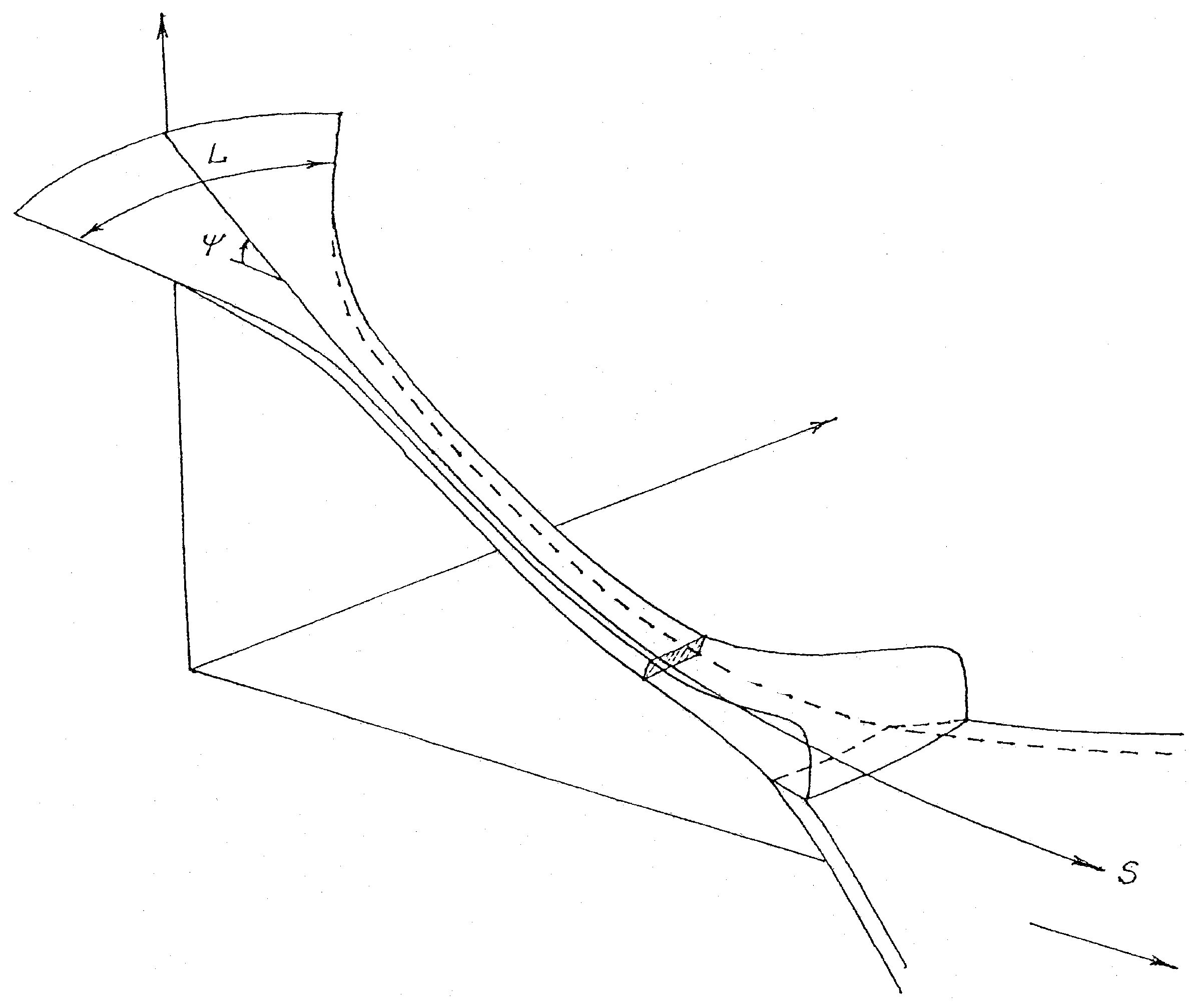
In deriving the system of Equations (1) and (2), we have assumed that the snow masses move in a channel with rectangular local cross-section that varies with the longitudinal coordinate along the channel axis. The structure of (1) also applies if the geometry of the channel cross-section varies but is prescribed as a function of the longitudinal coordinate. Here, t, S are the time and space coordinate along the avalanche trajectory on the bed (see Figure 1); $u(S,t)$, $F(S,t)$ are the unknown values of the S-component of snow velocity averaged over the full cross-section of the flow and the area of this cross-section, respectively; $L\left(S\right)$, $\psi \left(S\right)$ are the local width of the cross-section and local inclination of the channel axis; g is the gravity acceleration, $a(S,u)$ is the projection of the full acceleration (gravitational plus centrifugal) of the snow “particle” onto the direction normal to the bed. Recall that u is averaged over the cross-section and along the S-coordinate with averaging scale larger than the depth of the flow. k is the hydraulic resistance coefficient; $R=FL/(L^2+2F)$ is the so-called hydraulic radius, and r is the curvature radius of the channel axis. The values of $f_1$, $f_2$, q are specified as follows. We follow Grigorian [4] and Grigorian and Ostroumov [5] for the friction force $f_1$ on the bed surface and adopt the expression ([1], Note 2)

$$f_1=\left\{\begin{array}{cc}\mu a\left(1+{\displaystyle \frac{h}{L}}\right)\hfill & \mathrm{if}{\tau }_1\equiv \mu \rho ah\le {\tau }_{*},\hfill \\ {\displaystyle \frac{{\tau }_{*}}{\rho h}}\left(1+{\displaystyle \frac{2h}{L}}-{\displaystyle \frac{{\tau }_{*}}{L\mu \rho a}}\right)\hfill & \mathrm{if}{\tau }_1>{\tau }_{*},\hfill \end{array}\right.$$

(3)

where $\mu$ is the Coulomb friction law coefficient, $\rho$ is the density of the flowing snow, h is the local flow depth, and ${\tau }_{*}$ is the upper limit of the friction shear stress that appears in the modified friction law of Grigorian [4], expressed as ([1], Note 3)

$$\tau =\left\{\begin{array}{cc}\mu p_n\hfill & \mathrm{if}\mu p_n\le {\tau }_{*},\hfill \\ {\tau }_{*}\hfill & \mathrm{if}\mu p_n>{\tau }_{*},\hfill \end{array}\right.$$

(4)

with $p_n$ the normal pressure on the sliding surface.

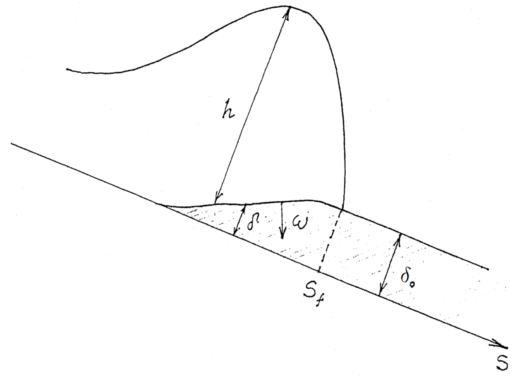
The quantities $f_2$ and q relate to entrainment of the (non-moving) snow cover at the frontal surface of moving snow. This process is difficult to model mathematically, and our approach is as follows. We suppose that the entrainment rate, represented by q, depends on the load p exerted on the snow cover by the moving snow. The kinematics of the erosion process are shown in Figure 2, where ${\delta }_0$ is the thickness of the (erodible) snow cover, $\delta$ is its thickness in the zone where that snow is gradually being entrained, and $\omega$ is the propagation velocity of the front where new snow is being eroded and mixed into the moving snow mass. Using the momentum and mass conservation laws, we can write ([1], Note 4)

$$\begin{array}{cc}\hfill \omega {\rho }_0& =(\omega -v){\rho }_1,\hfill \end{array}$$

(5)

$$\begin{array}{cc}\hfill \omega v{\rho }_0& =\left\{\begin{array}{cc}p-p_{*}\hfill & \mathrm{if} p>p_{*},\hfill \\ 0\hfill & \mathrm{if} p\le p_{*}\hfill \end{array}\right.\hfill \end{array}$$

(6)

where ${\rho }_0$ and ${\rho }_1$ are the densities of undisturbed new snow and eroded snow; $\omega$ and v are the interface-normal velocity components of the erosion front and of avalanching snow particles, $p_{*}$ is the strength of the snow cover, and p is the full pressure (hydrostatic plus dynamic) exerted on the bed (new snow) surface. Furthermore, we shall consider the case ${\rho }_1>{\rho }_0$.

The relations (5) and (6) lead to

$$\omega =\sqrt{\frac{p-p_{*}}{{\rho }_0(1-{\rho }_0/{\rho }_1)}}=\sigma \sqrt{\frac{p-p_{*}}{{\rho }_0}},\sigma \approx \mathrm{const}.,$$

(7)

with the parameter $\sigma$ characterizing the degree of snow compaction during the erosion process. The pressure p is expressed by the relation

$$p=\rho \left(ahcos\alpha +C{u}^{2}sin\alpha \right),\alpha =arctan\left(\frac{\partial \delta }{\partial S}\right),$$

(8)

where $h(S,t)$ and $\delta (S,t)$ are the local depth of moving snow and the local thickness of the erodible snow cover, respectively; C is an empirical constant. Using (7), we get the expression

$$q=\frac{\omega }{cos\alpha }\frac{{\rho }_0}{\rho }L=\left\{\begin{array}{cc}{\displaystyle \frac{\sigma L}{\rho cos\alpha }}\sqrt{(p-p_{*}){\rho }_0}\hfill & \mathrm{if} p>p_{*},\hfill \\ 0\hfill & \mathrm{if} p\le p_{*},\hfill \end{array}\right.$$

(9)

for the entrainment rate q. The average density $\rho$ is assumed to differ from ${\rho }_1$ in general. These considerations also lead to the following expression for the force contribution $f_2$ ([1], Note 5):

$$f_2=\left\{\begin{array}{cc}{\displaystyle \frac{qu}{F}}+a{\displaystyle \frac{\partial \delta }{\partial S}}\hfill & \mathrm{if} \delta >0,\hfill \\ 0\hfill & \mathrm{if} \delta =0,\hfill \end{array}\right.$$

(10)

where the condition $\delta =0$ means that the new-snow layer is completely eroded and entrained at a certain distance behind the avalanche front.

An alternative expression for q can be derived by connecting the snow erosion rate to the shear forces, leading to an empirical relation of the type

$$q=\xi {\left[\rho \left(u^2-u_{*}^2\right)\right]}^n,\xi ,n,u_{*}=\mathrm{const}..$$

(11)

This alternative formula can easily be implemented in the mathematical model, but we will not discuss this in detail here.

Finally, we have the set of relations (1)–(3), (8)–(10), giving the closed mathematical formulation of the model. Before they can be used to solve a given problem, it remains to formulate the initial and boundary conditions.

The initial conditions are

$$u(S,0)=u_0\left(S\right),F(S,0)=F_0\left(S\right),\delta (S,0)={\delta }_0\left(S\right),$$

(12)

where the functions $u_0\left(S\right)$, $F_0\left(S\right)$, and ${\delta }_0\left(S\right)$ are to be specified for each case under consideration.

The boundary conditions describe the motion of the front and the “tail” part of the snow flow. Even though the moving snow mass not only has a sharp frontal boundary but also a tail moving down the mountain side, we suppose that the latter boundary has limited importance for the dynamics of the main snow mass. Therefore, we adopt a simpler scheme with the tail of the avalanche at rest. In other words, we will set the tail boundary conditions as

$$u(S_0,0)=0,F(S_0,0)=0$$

(13)

where $S_0$ is the (constant) coordinate of the avalanche tail.

The boundary conditions at the avalanche front are evident:

$$u(S_f,t)=w,w=\frac{\mathrm{d}{S}_f\left(t\right)}{\mathrm{d}t},F(S_f,t)=0,\delta (S_f,t)={\delta }_0\left(S_f\right),$$

(14)

where $S_f\left(t\right)$ is the coordinate of the front—a function of t to be determined in the course of solving the problem.

This completes the full mathematical formulation of the initial–boundary value problem of snow avalanche dynamics.

Now we consider a special case of the problem where the channel is infinitely wide ($L\to \infty$), making the motion effectively two-dimensional, and the slope is devoid of erodible snow. Such a simplification of the problem allows to obtain results in a form suitable for analysis and parametric comparisons, which serve as guideposts in more complicated cases.

In this case, we have the differential equations

$$\frac{\partial u}{\partial t}+u\frac{\partial u}{\partial S}=gsin\psi -f\mathrm{sign}\left(u\right)-\frac{k{u}^2}{R}\mathrm{sign}\left(u\right)-\frac{1}{2h}\frac{\partial \left(a{h}^2\right)}{\partial S},$$

(15)

$$\frac{\partial h}{\partial t}+\frac{\partial \left(uh\right)}{\partial S}=0,$$

(16)

initial conditions

$$u(S,0)=u_0\left(S\right),h(S,0)=h_0\left(S\right),$$

(17)

with $S\in [S_0,S_f\left(0\right)]$, and the boundary conditions

$$u(S_0,t)=0,h(S_0,t)=0,$$

(18)

$$u(S_f\left(t\right),t)=w\left(t\right),h(S_f\left(t\right),t)=0.$$

(19)

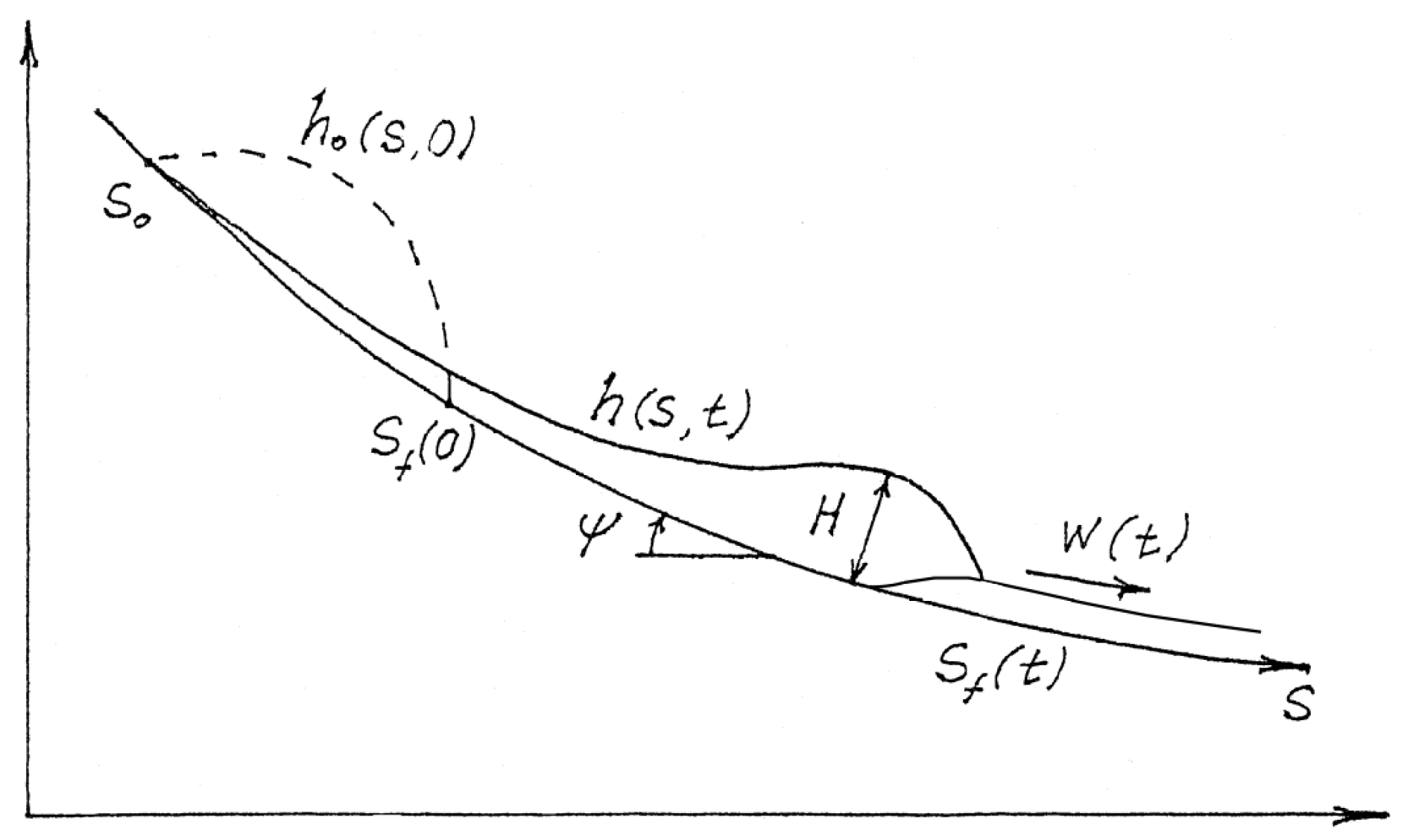
Here, again, t and S are the time and the space coordinate along the avalanche path (see Figure 3), $S_f\left(t\right)$ is the coordinate of the avalanche front, etc.; $h(S,t)$ is the local depth of the avalanche; $u_0\left(S\right)$, $h_0\left(S\right)$ are the initial distributions of $u(S,t)$ and $h(S,t)$, respectively; f is the retarding acceleration given by the relation

$$f=\left\{\begin{array}{cc}\mu a\hfill & \mathrm{if} {\tau }_1\equiv \mu \rho ah<{\tau }_{*},\hfill \\ {\displaystyle \frac{{\tau }_{*}}{\rho h}}\hfill & \mathrm{if} {\tau }_1\ge {\tau }_{*},\hfill \end{array}\right.$$

(20)

where again $\mu$ is the Coulomb friction coefficient, $\rho$ is the density of flowing snow, and ${\tau }_{*}$ is the upper limit of the frictional stress $\tau$ on the bed surface, as specified in the modified friction law proposed in [4]. In the mathematical formulation of the problem (15)–(20), the set of parameters $\psi \left(S\right)$, $u_0\left(S\right)$, $h_0\left(S\right)$, $\mu$, k, $\rho$, ${\tau }_{*}$, is assumed known. The function $\psi \left(S\right)$ describes the geometry of the slope and is known if the topography of the slope is available. The other quantities in this parameter set have to be estimated from the mechanical properties of snow, which depend on climatic and geographical factors and—in the case of $u_0\left(S\right)$ and $h_0\left(S\right)$—on the probable and admissible initial distributions of u and h.

The problem formulated in terms of the full model can usually only be solved numerically on a computer ([1], Note 6). This is recommended for “precise” calculations when detailed information about the input data ($\psi \left(S\right)$, k, etc.) is available and the mathematical predictions are to be calculated as exactly as possible. The formulation (15)–(20) provides the necessary tools for such work.

However, in many real cases, there is insufficient information available on $\psi \left(S\right)$, $\mu$, and other input quantities. Moreover, one often needs a simpler mathematical instrument for estimates—either an explicit formula or a simple computational procedure that can be applied without a powerful computer. For such purposes, we can construct different classes of simplified models, and those derivations are the topic of the following parts of this work.

3. A Simplified Version of the Full Model

A possible simplification procedure, considered initially in [6], is as follows. On the right-hand side of (1), we neglect the third and last term and rewrite the resulting equation in a Lagrangian coordinate system as

$$S=S(\xi ,t),u=\frac{\partial S}{\partial t},$$

(21)

where $\xi$ is the Lagrangian coordinate. This transforms (1) into

$$\frac{1}{2}\frac{\partial u^2}{\partial S}=gsin\psi -f\mathrm{sign}\left(u\right).$$

(22)

The second step of the simplification procedure introduces the integrated form of the mass conservation law instead of its differential form (16). Integration of $h(S,t)$ over the coordinate S leads to the relation

$$F\left(t\right)={\int }_{S_0}^{S_f\left(t\right)}h(S,t)\mathrm{d}S=\varkappa Hl=\mathrm{const}.\equiv F_0,$$

(23)

where $F_0=F\left(0\right)$, $H={max}_S\left(h(S,t)\right)$, and $l=S_f\left(t\right)-S_0$. $\varkappa$ is a parameter characterizing the“fullness” of the graph of $h(S,t)$. Now we make the crucial and plausible assumption that $\varkappa$ is constant ([1], Note 7). Of course, $\varkappa$ changes over time but, as will be demonstrated by comparing numerical results obtained from the full and simplified models, the deviations of $\varkappa$ from a constant value are not dramatic; therefore, this hypothesis looks acceptable for estimations.

To evaluate the model (21)–(23) with simple calculation tools, one can divide the avalanche path into several segments, introducing the dividing points $S_0$, $S_1$, $S_2,\dots ,S_N$ so that changes of $\psi \left(S\right)$ can be neglected within each segment $S_i\le S\le S_{i+1}$. This allows us to integrate (22) over $[S_i,S_{i+1}]$, where we get the relation

$$u^2\left(S\right)=u^2\left(S_i\right)+2(S-S_i)\left[g{\overline{(sin\psi )}}_i-{\overline{f}}_i\right],$$

(24)

where

$${\overline{(sin\psi )}}_i=\frac{1}{S_{i+1}-S_i}{\int }_{S_i}^{S_{i+1}}sin\psi \left(S\right)\mathrm{d}S,{\overline{f}}_i=\frac{1}{S_{i+1}-S_i}{\int }_{S_i}^{S_{i+1}}f\left(S\right)\mathrm{d}S$$

(25)

(we consider only the case $u>0$, $\mathrm{sign}\left(u\right)=1$). To calculate the velocity u from (24), we need information about h to evaluate (25). As calculations with the full model demonstrate, the important unknowns of avalanche motion—velocity, depth, and runout distance—are mainly determined by the flow properties in the zone near the coordinate with the maximum value of h. The full-model calculations show that this region is closely attached to the avalanche front and that the Lagrangian coordinate of the phase with $h\left(S\left(\xi \right)\right)={max}_S\left(h(S,t)\right)$ changes little over time. For this reason, we can further simplify the calculations by supposing that this coordinate remains unchanged in time and coincides with the Lagrangian coordinate of the avalanche front. All these considerations allow us to use the value $H=max\left(h\right)$ instead of h and calculate l by the relation

$$l=S-S_0,$$

(26)

substituting S for $S_f$ because S-coordinates in the dynamically most significant zone near the cross-section with $H\approx max\left(h\right)$ are close to $S_f$. In [6], values in the range $\varkappa \approx 0.3$–0.4 are recommended in cases where the geometry of the slope changes smoothly with S.

Of course, to assess the accuracy of the simplified model presented here, one needs to compare parallel calculations for the same problem using the full and the simplified model. This was done, and the results are presented in the next section.

4. Comparison of Computations with the Full and Simplified Models

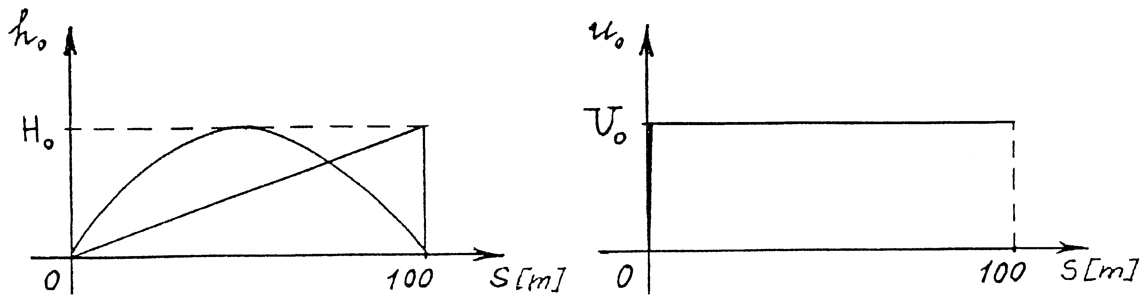
The calculations with the full model were performed in a simple geometry with $\psi =\mathrm{const}$. On the interval $[S_0=0,S_f\left(0\right)=100\mathrm{m}]$, different initial distributions $h_0\left(S\right)$, $u_0\left(S\right)$ were prescribed, and different combinations of the values of the parameters $\mu$, k, $\rho$, ${\tau }_{*}$, and $\psi$ were tested.

Table 1. The set of numerical values of the problem parameters for tested variants ([1], Note 8).

Variant N	$\mathit{\mu }$ —	k —	${\mathit{\tau }}_{*}$ kPa	$\mathit{\rho }$ $\mathbf{kg}{\mathbf{m}}^{-3}$	$\mathit{\psi }$ ${}^{\circ }$	${\mathit{U}}_0$ $\mathbf{m}{\mathbf{s}}^{-1}$	${\mathit{H}}_0$ m	Profile ${\mathit{h}}_0\left(\mathit{s}\right)$
1	0.5	0.02	10	500	30	10	1	parabola
2	0.5	0.02	10	500	30	1	10	parabola
3	0.5	0.02	10	500	30	10	10	triangle
4	0.5	0.02	10	500	30	10	1	triangle
5	0.5	0.02	10	500	30	10	1	parabola
6	0.5	0.02	10	500	30	10	60	triangle
7	0.5	0.02	10	500	46	1	10	parabola
8	0.25	0.02	10	500	30	1	10	parabola
9	0.5	0.06	10	500	30	1	10	parabola
10	0.5	0.02	2.5	500	30	1	10	parabola

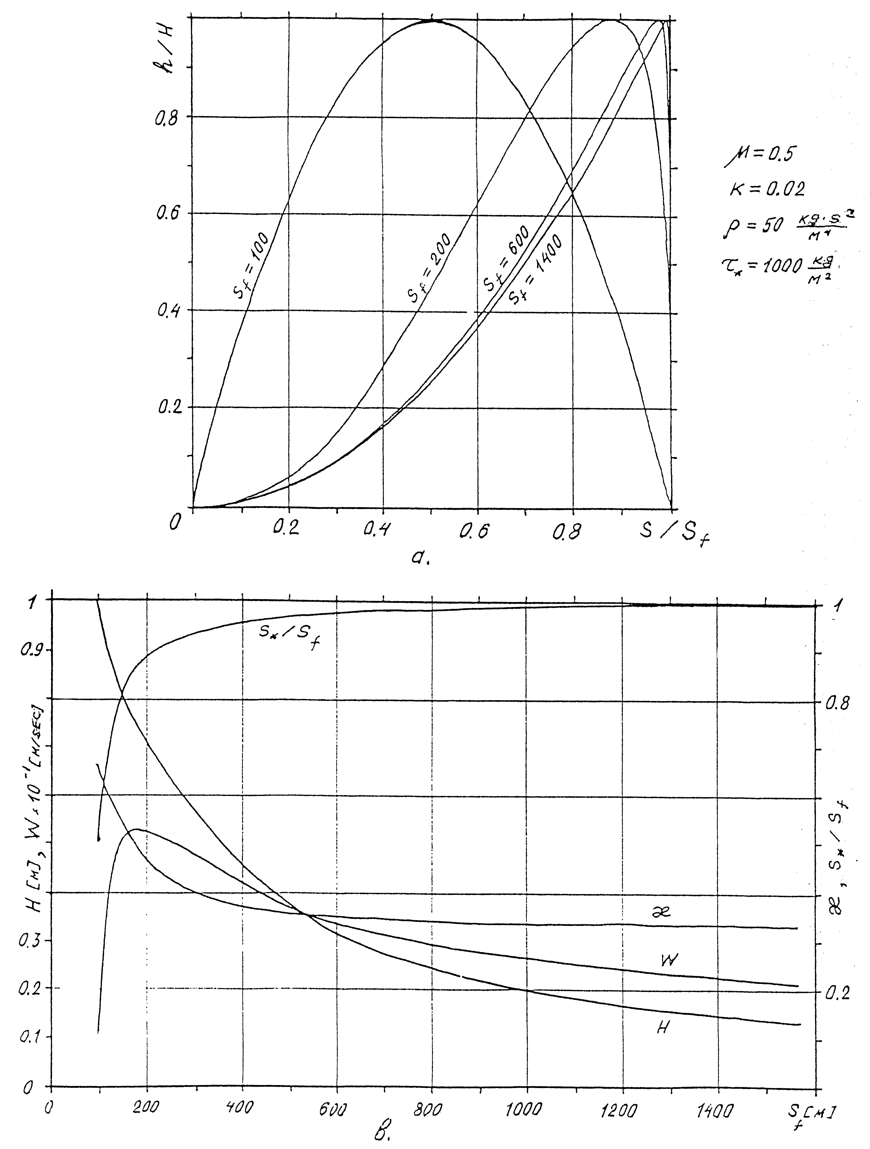
details the parameter values for the different variants. The basic variant was $\psi ={30}^{\circ }$, $\mu =0.5$, $k=0.02$, $\rho =500\mathrm{kg}{\mathrm{m}}^{-3}$, ${\tau }_{*}=10$ kPa ([1], Note 8). $h_0\left(S\right)$ was prescribed as triangular or parabolic forms with different values of $H_0$; for $u_0\left(0\right)$, a uniform distribution was used (see Figure 4). Figure 5a presents the distribution of $h/H$ as a function of S in different stages of the motion. Figure 5b plots the evolution of $\varkappa$, H, w, and $S_{*}/S_f$ against $S_f$, where $S_{*}$ is the S-coordinate of the point where $h=max\left(h\right)=H$. All these data relate to the basic variant. Figures S2.1–S2.9 in SMD 2 illustrate analogous results for other variants.

The common feature of the solutions for all the variants is their fast approach towards an asymptotic form, independent of the initial distribution. The asymptotic distribution of h can be described approximately by the relation $h/H={(S/S_f)}^2$, and H, w and $S_{*}/S_f$ become smooth and slowly varying functions of t with $S_{*}/S_f\to 1$, $\varkappa \to 0.36$ for all the variants calculated.

Note that the asymptotic behavior of the solution emerges after the avalanche body has spread to the point where $H<h_{*}\equiv {\tau }_{*}/\left({\rho }_a\mu \right)$, so that the Coulomb friction law governs the entire avalanche body. Before this stage, significant changes in $\varkappa$ and $S_{*}/S_f$ are visible, and the character of these changes depends essentially on the initial data.

We can conclude that the asymptotic simplification of the flow structure with $\varkappa =\mathrm{const}.$, $S_{*}/S_f=\mathrm{const}.\approx 1$ will occur in cases with slowly changing slope geometry, and for this very case the simplified model is acceptable for simple estimations. In

Table 2. The results of calculations with the full model (Section 2), the simplified model of Section 3 (formulas (23) and (24)), and the improved simplified model described in Section 5 (formulas (36), (39) and (40)) are presented in terms of the flow depth H and the front velocity w as functions of the front position $S_f$. For the simplified models, the value of the shape factor was always chosen as $\varkappa =0.36$ ([1], Note 9).

Variant	Sf	H(m)		w(ms−1)
N	(m)	Full Model	Formula (23)	Full Model	Formula (24)	Formula (36)	Formula (40)	Formula (39)
1	100	1.000		1.00	1.00	1.00	(10.64)	(7.8)
	200	0.722	0.929	5.23	11.49	5.98	5.862	5.51
	600	0.323	0.309	3.37	25.61	3.21	3.203	3.18
	1000	0.200	0.185	2.60	34.35	2.60	2.469	2.47
	1400	0.416	0.132	2.22	41.27	2.09	2.080	2.08
2	100	10.000		1.00	1.00	1.00	—	(24.65)
	200	4.733	9.290	18.48	25.64	23.45	—	17.43
	400	2.900	3.620	13.50	36.39	21.13	14.62	12.32
	600	1.973	3.090	8.46	39.83	10.96	10.78	10.07
	1000	1.607	1.850	7.60	45.95	8.01	7.78	7.80
	1400	1.272	1.320	6.64	51.35	6.68	6.67	6.59
7	100	10.00	18.52	1.0	1.00	1.00	—	(58.17)
	200	6.25	9.29	28.0	32.00	30.12	—	41.13
	400	4.00	4.63	28.5	51.00	30.52	34.49	29.10
	600	3.00	3.09	25.5	64.00	25.82	25.45	23.75
	1000	2.20	1.85	21.2	84.14	18.88	18.84	18.38
	1400	1.50	1.32	16.0	100.0	15.74	15.73	15.52
	2000	1.00	0.93	14.0	120.0	13.09	13.08	13.01
	2500	0.75	0.74	12.0	134.0	11.75	11.68	11.63
8	100	10.00	18.52	1.0	1.00	1.00	—	(50.72)
	200	4.8	9.29	21.5	25.64	21.6	—	35.86
	400	3.5	4.63	23.5	42.10	26.60	30.07	25.36
	600	2.9	3.09	21.6	53.67	22.51	22.18	20.69
	1000	2.0	1.85	17.0	71.63	16.47	16.42	16.03
	1400	1.7	1.54	14.7	78.83	14.89	14.88	14.63
9	100	10.00	18.52	1.0	1.00	1.00	—	(14.23)
	200	4.90	9.29	13.5	25.64	18.41	12.84	10.06
	400	2.70	4.63	5.9	36.39	7.92	7.49	7.11
	600	2.25	3.09	5.3	39.83	5.95	5.94	5.81
	1000	1.65	1.85	4.8	45.95	4.54	4.54	4.50
	2000	1.50	1.54	4.2	48.70	4.14	4.14	4.11

, the results of calculations with the full and simplified model are presented in terms of w and H as functions of $S_f$. One can see that the simplified theory gives acceptable accuracy for H and overestimates the values of the front velocity w. This last effect is mainly due to our neglecting the resistance term $-k{u}^2/h$ in the equation of motion of the simplified model and indicates the necessity of improving the simplified theory. Such an improvement will be presented in the following section.

5. Improvement of the Simplified Model

Including in the momentum equation the collisional term $-k{u}^2/h$ and using all other simplifying considerations introduced in the previous section, we get the relations

$$\frac{1}{2}\frac{\partial u^2}{\partial S}=gsin\psi -f-\frac{k{u}^2}{H},$$

(27)

$$H=\frac{F_o}{\varkappa l}.$$

(28)

Introducing the definitions

$$A\equiv \left\{\begin{array}{cc}2(gsin\psi -\mu a)\hfill & \mathrm{if} \tau \equiv \mu \rho aH<{\tau }_{*},\hfill \\ 2gsin\psi \hfill & \mathrm{if} \tau \ge {\tau }_{*},\hfill \end{array}\right.$$

(29)

$$B\equiv \frac{2k\varkappa }{F_0},$$

(30)

$$D\equiv \left\{\begin{array}{cc}0\hfill & \mathrm{if} \tau <{\tau }_{*},\hfill \\ {\displaystyle \frac{2{\tau }_{*}\varkappa }{\rho F_0}}\hfill & \mathrm{if} \tau \ge {\tau }_{*},\hfill \end{array}\right.$$

(31)

we can rewrite (27) in the form

$$\frac{\partial u^2}{\partial S}=A-B{u}^{2}S-DS.$$

(32)

The solution of (32) on the segments $S\in [S_i,S_{i+1}]$ with initial condition

$$u\left(S_i\right)=u_{0,i}$$

(33)

is given by the relation ([1], Note 10)

$$u\left(S\right)=\sqrt{-{\displaystyle \frac{D}{B}}+Aexp\left(-{\displaystyle \frac{B{S}^2}{2}}\right){\int }_{S_i}^{S}exp\left({\displaystyle \frac{B{x}^2}{2}}\mathrm{d}x\right)+\left(u_{0,i}^2+{\displaystyle \frac{D}{B}}\right)exp\left({\displaystyle \frac{B}{2}}(S_i^2-S^2)\right)}.$$

(34)

When calculating the coefficients A, B, and D, one should use the average of $\psi$ over the interval $[S_i,S_{i+1}]$.

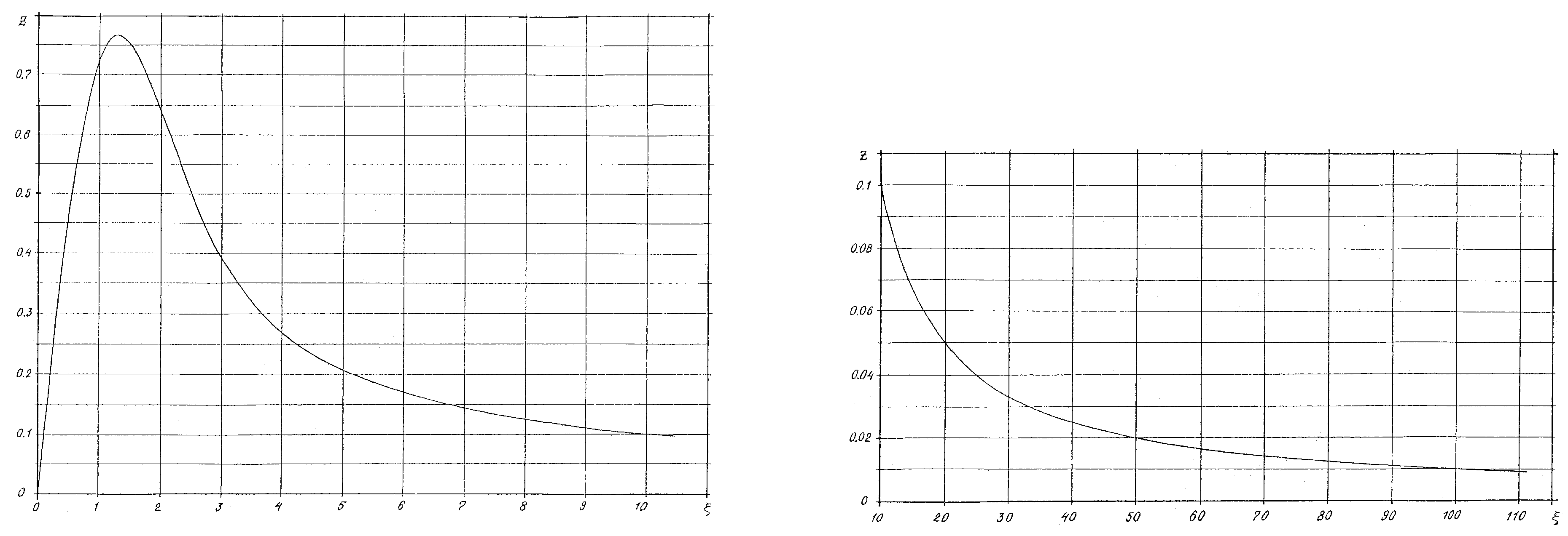
Defining the function

$$Z\left(\xi \right)\equiv exp\left(-{\xi }^2/2\right){\int }_0^{\xi }exp\left(x^2/2\right)\mathrm{d}x$$

(35)

and setting $\xi \equiv S\sqrt{B}$, we get

$$u\left(S\right)=\sqrt{-{\displaystyle \frac{D}{B}}+{\displaystyle \frac{A}{\sqrt{B}}}Z\left(\sqrt{B}S\right)+\left(u_{0,i}^2+{\displaystyle \frac{D}{B}}-{\displaystyle \frac{A}{\sqrt{B}}}Z\left(\sqrt{B}{S}_i\right)\right)exp\left({\displaystyle \frac{B}{2}}(S_i^2-S^2)\right)}$$

(36)

The graph of $Z\left(\xi \right)$ is shown in Figure 6.

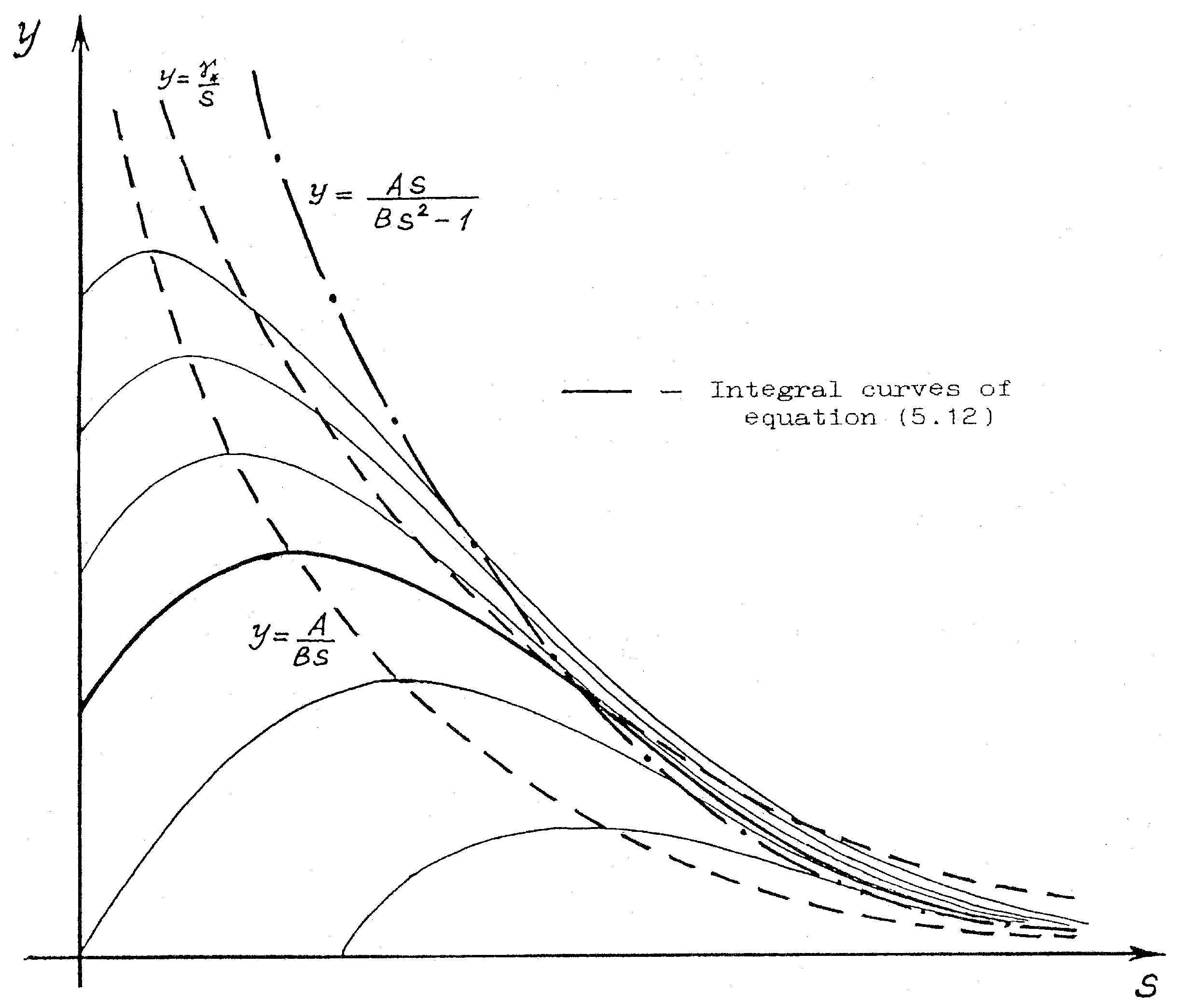
Consider now the qualitative features of solutions of (32). Using a new variable y,

$$y=u^2+D/B,$$

(37)

we have, instead of (32), the equation

$$y^{\prime }=A-BSy,$$

(38)

and as $u^2=y-D/B\ge 0$, we will be interested only in solutions of (38) satisfying the conditions $y\ge D/B\ge 0.$

On the y-S plane, the hyperbolas $yS=\gamma =\mathrm{const}.$ ([1], Note 11) are the isoclines of (38), i.e., the lines along which $y^{\prime }=\mathrm{const}.$ On the hyperbolas

$$y=\frac{A}{BS},$$

(39)

we have $y’=0$, so all the solutions have extrema there (more precisley, these are maxima, for if $\gamma <A/B$ then $y^{\prime }>0$ and at $\gamma >A/B$$y^{\prime }<0$). As a result, we can visualize the integral curves of Equation (38) as shown in Figure 7. Depending on the initial data, when $S\to \infty$ an integral curve tends to the hyperbola (39), $yS=A/B$, either monotonically or after some initial rise to a maximum value of y. It can easily be shown that $y^{″}=0$ on the curve

$$y=\frac{AS}{B{S}^2-1}$$

(40)

and that, at any given point of (40) with coordinate $S=S_{*}$, a solution of (38) touches some hyperbola $yS={\gamma }_{*}$ depending on the initial data. For $S>S_{*}$, this solution becomes “captured” between the curve (40) and the hyperbola $yS={\gamma }_{*}$. This leads to simple estimates for large values of S:

$$\frac{A}{BS}<\frac{AS}{B{S}^2-1}<y<\frac{{\gamma }_{*}}{S}.$$

(41)

On the basis of this improved model, a series of calculations have been performed with the same parameter values as for the non-improved model, and the results are shown in Table 2, illustrating the performance of the improved model compared to the “exact” results of the full model. The correspondence between these two sets of results is very good over a wide range of the key parameters of the problem. At large values of S, even the simplest relation (39) delivers estimations of high accuracy. Note that all these calculations were performed for $\varkappa =0.36$. This value, thus, can be recommended for practical use over a wide range of parameters.

6. The Simplest Model for Rough Estimations

In the literature, one can find many articles that use a very simple scheme for snow avalanche dynamics. In this scheme, the avalanche is considered as a material point, neglecting the spatial extent of the flowing snow mass and its changes in time. Here, we will consider the problem in this case and establish what kind of assumptions are needed to derive such a model from the “exact” one. The main differential equations of the material point model are as follows:

$$\frac{\mathrm{d}S}{\mathrm{d}u}=u,m\frac{\mathrm{d}u}{\mathrm{d}t}=mgsin\psi -r,$$

(42)

where m is the total mass, which is assumed to be constant, r is the resistance force between the moving body and the underlying base surface, and other denotations are as before. We can write the relation

$$m=\rho Hlb,$$

(43)

where $\rho$ is the snow density (assumed constant), H, l, b are the height, length, and width of the avalanche body, respectively. For the resistance r, we have

$$r=lb\tau ,$$

(44)

where $\tau$ is the average frictional stress on the bed surface. So, we reduce (42)–(44) to

$$\frac{\mathrm{d}S}{\mathrm{d}t}=u,\frac{\mathrm{d}u}{\mathrm{d}t}=gsin\psi -{\displaystyle \frac{\tau }{\rho H}},$$

(45)

and it is obvious that, to derive Equation (45) from the corresponding momentum Equation (1) of the full model, we must neglect the term representing the gradient of normal force acting at the cross-section of the avalanche body ([1], Note 12), $(\rho g/2F)\partial F/\partial S$, and include the hydrodynamic resistance term, $-k\rho u^2/R$, in the expression for $\tau$, if desired. Up to this point, there is no difference between the simplified model of Section 3 and that under consideration here. Such a difference appears when we look at the next simplification in this simplest point-mass model, which assumes the flow depth H to be constant. As calculations with the full or simplified model reveal, H varies significantly in the course of the avalanche propagation along the mountain slope. One may, nevertheless, hope that it is admissible for rough estimations to use $H=\mathrm{const}$.

Consider now the evaluation of the simplest model for several hypotheses about the bed shear stress $\tau$.

6.1. Solutions for the Coulomb and Voellmy Friction Laws

In point-mass model calculations ([1], Note 13), often the Coulomb friction law is used, with $\tau$ expressed as

$$\tau =\mu p_n,p_n=\rho gHcos\psi ,$$

(46)

in which the hydrodynamic term (quadratic in u) is neglected. In this case, the problem is solved by quadrature:

$$u^2=u_0^2+2g{\int }_{S_0}^S\left[sin\psi \left(\xi \right)-ucos\psi \left(\xi \right)\right]\mathrm{d}\xi ,$$

(47)

$$u_{0}t={\int }_{S_0}^S{\displaystyle \frac{\mathrm{d}\xi }{\sqrt{1+\frac{2g}{u_0^2}{\int }_{S_0}^{\xi }\left[sin\psi \left({\xi }^{\prime }\right)-\mu cos\psi \left({\xi }^{\prime }\right)\right]\mathrm{d}{\xi }^{\prime }}}},$$

(48)

where $S_0$, $u_0$ are the initial position and velocity of the avalanche body.

For a given slope geometry, the right-hand sides of (47) and (48) are known functions of S (as $\psi \left(S\right)$ is known). So, the numerical evaluation of these expressions reduces to rather simple calculations. Note that if the slope is steep enough, i.e., $sin\psi -\mu cos\psi >0$, the avalanche motion will accelerate in time. In the opposite case, the motion decelerates and even stops on the slope if the inclined part of the trajectory is long enough.

To obtain explicit formulas for analyzing the avalanche behavior, we consider an avalanche path consisting of two segments, the first inclined at an angle ${\psi }_1=\mathrm{const}.$ and the second horizontal (${\psi }_2=0$). Using (47) and assuming $u_0\ge 0$, we have ([1], Note 14)

$$u=u_0\sqrt{1+{\displaystyle \frac{2g(S-S_0)}{u_0^2}}(sin{\psi }_1-\mu cos{\psi }_1)}.$$

(49)

With $l_1\equiv S_1-S_0$, where $S_1$ is the coordinate of the end of the first slope segment, we get the initial velocity in the second segment as

$$u_1=u_0\sqrt{1+{\displaystyle \frac{2g{l}_1}{u_0^2}}(sin{\psi }_1-\mu cos{\psi }_1)}.$$

(50)

Using (47) in this segment with (50), instead of $u_0$, and substituting ${\psi }_2=0$, we have ([1], Note 15)

$$u^2=u_1^2-2g\mu (S-S_1).$$

(51)

In the second segment, the avalanche decelerates and completely stops at some distance $S_2$. So, for this distance, we have (substituting $u=0$, $S=S_2$ in (51))

$$l_2\equiv S_2-S_1=\frac{u_1^2}{2g\mu }.$$

(52)

Note that this runout distance $l_2$ does not depend at all on the avalanche size.

Using (50) and (52) and the definition of $l_1$, we obtain the full runout distance $L=S_2-S_0$ as ([1], Note 16)

$$L=S_2-S_0=\frac{u_0^2}{2g\mu }+\left(1+\frac{sin{\psi }_1}{\mu }-cos{\psi }_1\right)l_1.$$

(53)

If $sin{\psi }_1-\mu cos{\psi }_1<0$, the avalanche may stop on the slope; in the opposite case, it runs out on the horizontal path segment.

We can now easily extend this simplest model with a resistance term that is quadratic in the velocity. In the inclined segment of the path, we have (assuming $u_0\ge 0$) ([1], Note 17)

$$u=\sqrt{{\displaystyle \frac{gH}{k}}(sin{\psi }_1-\mu cos{\psi }_1)+\left[u_0^2+{\displaystyle \frac{gH}{k}}(sin{\psi }_1-\mu cos{\psi }_1)\right]exp\left(-{\displaystyle \frac{2k}{H}}(S-S_0)\right)},$$

(54)

$$u_1=\sqrt{{\displaystyle \frac{gH}{k}}(sin{\psi }_1-\mu cos{\psi }_1)+\left[u_0^2+{\displaystyle \frac{gH}{k}}(sin{\psi }_1-\mu cos{\psi }_1)\right]exp\left(-{\displaystyle \frac{2k{l}_1}{H}}\right)}$$

(55)

instead of (49) and (50).

On the horizontal path segment, we find

$$u=\sqrt{-{\displaystyle \frac{\mu gH}{k}}+\left[u_1^2+{\displaystyle \frac{\mu gH}{k}}\right]exp\left(-{\displaystyle \frac{2k}{H}}(S-S_1)\right)}.$$

(56)

So, if we set $u=0$ here, we get

$$l_2\equiv S_2-S_1=\frac{H}{2k}ln\left[1+{\displaystyle \frac{sin{\psi }_1}{\mu }}-cos{\psi }_1+\left({\displaystyle \frac{k{u}_0^2}{\mu gH}}-{\displaystyle \frac{sin{\psi }_1}{\mu }}+cos{\psi }_1\right)exp(-2k{l}_1/H)\right]$$

instead of (52).

Finally, we have for the full runout distance ([1], Notes 16 and 18)

$$L=\frac{H}{2k}ln\left[1+{\displaystyle \frac{sin{\psi }_1}{\mu }}-cos{\psi }_1+\left({\displaystyle \frac{k{u}_0^2}{\mu gH}}-{\displaystyle \frac{sin{\psi }_1}{\mu }}+cos{\psi }_1\right)exp(-2k{l}_1/H)\right]+l_1.$$

(57)

When $k\to 0$, Equation (54)–(57) reduce to (49)–(53), as they should.

6.2. Solution with the Stress-Limited Friction Law

Consider now the case of very big avalanches for which the snow depth H almost everywhere in the avalanche body exceeds the critical value $H_{*}={\tau }_{*}/(\mu \rho cos\psi )$ beyond which the friction law $\tau ={\tau }_{*}=\mathrm{const}.$ is applicable instead of the Coulomb law ([1], Note 13). In this case, after integrating (44), we have the following relations in the initial segment of the avalanche path:

$$u=u_0+\left(gsin{\psi }_1-\frac{{\tau }_{*}}{\rho H}\right)t,S-S_0=u_{0}t+\frac{1}{2}\left(gsin{\psi }_1-\frac{{\tau }_{*}}{\rho H}\right)t^2.$$

(58)

At the mountain foot, at $S-S_0=S_1-S_0=l_1$, we have

$$t=t_1,u=u_1=u_0+\left(gsin{\psi }_1-\frac{{\tau }_{*}}{\rho H}\right)t_1,l_1=u_0{t}_1+\frac{1}{2}\left(gsin{\psi }_1-\frac{{\tau }_{*}}{\rho H}\right)t_1^2,$$

(59)

and

$$\begin{array}{cc}\hfill t_1& ={\displaystyle \frac{\sqrt{u_0^2+2\left(gsin{\psi }_1-{\displaystyle \frac{{\tau }_{*}}{\rho H}}\right)l_1}-u_0}{gsin{\psi }_1-{\displaystyle \frac{{\tau }_{*}}{\rho H}}}},\hfill \\ \hfill u_1& =\sqrt{u_0^2+2\left(gsin{\psi }_1-{\displaystyle \frac{{\tau }_{*}}{\rho H}}\right)l_1}.\hfill \end{array}$$

(60)

For the second (horizontal) part, we have

$$u=u_1-\frac{{\tau }_{*}}{\rho H}t,S-S_1=u_{1}t-\frac{{\tau }_{*}}{2\rho H}{t}^2,$$

(61)

and at $S-S_1=S_2-S_1=l_2$, where $u=0$, we obtain

$$t=t_2=\frac{\rho H{u}_1}{{\tau }_{*}}=\frac{\rho H}{{\tau }_{*}}\sqrt{u_0^2+2\left(gsin{\psi }_1-{\displaystyle \frac{{\tau }_{*}}{\rho H}}\right)l_1},$$

(62)

$$l_2=u_1{t}_2-\frac{{\tau }_{*}}{2\rho H}{t}_2^2=\frac{\rho H}{2{\tau }_{*}}\left(u_0^2+2g{l}_{1}sin{\psi }_1\right)-l_1.$$

(63)

The full distance $L=l_1+l_2$ is given by the formula ([1], Notes 16 and 19)

$$L=\frac{\rho H}{2{\tau }_{*}}\left(u_0^2+2g{l}_{1}sin{\psi }_1\right).$$

(64)

An important feature of the relations obtained in this case is their pronounced dependence on the avalanche size H. The dependence of the runout distance L on H is particularly interesting: The bigger (deeper) the avalanche is, the longer is its runout. In this respect, big avalanches governed by the limited-stress friction law with $\tau ={\tau }_{*}=\mathrm{const}.$ differ significantly from small avalanches governed by the classic Coulomb law.

This conclusion is, of course, valid not only for the simplest model considered here but also for the “exact” ones as it is a direct consequence of the physical difference between these two friction laws. The restriction of the bed shear stress to the limiting value ${\tau }_{*}$ leads to extremely high mobility of the snow flow on the mountain slope and the horizontal plane, with a dramatic rise of runout distance with increasing avalanche size.

It is also interesting to see how these results are modified when hydraulic resistance, represented by the term $-k{u}^2/H$, is included in Equation (44). In this case, integration over the initial path segment gives

$$u^2=u_{*}^2+\left(u_0^2-u_{*}^2\right)exp\left[-\frac{2k}{H}(S-S_0)\right],u_{*}^2\equiv \frac{H}{k}\left(gsin{\psi }_1-\frac{{\tau }_{*}}{\rho H}\right),$$

(65)

$$u_1^2=u_{*}^2+\left(u_0^2-u_{*}^2\right)exp\left(-\frac{2k}{H}{l}_1\right),$$

(66)

and in the second segment, one obtains ([1], Note 20)

$$u^2=\left(u_{**}^2+u_1^2\right)exp\left[-\frac{2k}{H}(S-S_1)\right]-u_{**}^2,u_{**}^2\equiv \frac{{\tau }_{*}}{\rho k}.$$

(67)

For the runout distance $S_2-S_1=l_2$, (67) and $u\left(S_2\right)=0$ lead to

$$\begin{array}{cc}\hfill l_2& =\frac{H}{2k}ln\left(\frac{u_1^2}{u_{**}^2}+1\right)\hfill \\ \hfill & =\frac{H}{2k}ln\left\{1+\frac{\rho H}{{\tau }_{*}}\left(gsin{\psi }_1-\frac{{\tau }_{*}}{\rho H}\right)+\frac{\rho k}{{\tau }_{*}}\left[u_0^2-\frac{H}{k}\left(gsin{\psi }_1-\frac{{\tau }_{*}}{\rho H}\right)\right]exp\left(-\frac{2k}{H}{l}_1\right)\right\}.\hfill \end{array}$$

(68)

Taking the limit $k\to 0$ in (68), one retrieves (63).

The strong dependence of $l_2$ on avalanche size H given by (68) is obvious, and all the conclusions relating to the properties of big avalanches made above in the simplest case with $k=0$ remain valid. However, the hydraulic resistance term significantly modifies the relationships (63) and (64) between runout distance and avalanche size H: They are no longer linear since Equation (68) contains logarithmic and exponential terms. As a result, the runout $l_2$ rises much more slowly with H than is predicted by the linear relations (63) and (64).

Consider a numerical example with the following parameter values ([1], Note 8): $k=0.02$; ${\tau }_{*}=10$ kPa; $\rho =500\mathrm{kg}{\mathrm{m}}^{-3}$; $\mu =0.5$; $sin\psi =0.5$; $g=10$,m/s${}^2$; $l_1=1000$ m; $H=5$ m; $u_0=0$. The Coulomb friction law (53) gives $l_2/l_1=0.137$, $l_2=137$ m. In the case of the limited-stress friction law, the relation (63) gives $l_2/l_1=0.25$, $l_2=250$ m. In this case, the lower limit on the flow depth for the shear stress to be limited by ${\tau }_{*}$ is $H_{*}={\tau }_{*}/\left(\mu \rho g\right)=4.62$ m. Thus, the value $H=5$ m used in the calculations is only slightly above $H_{*}$. This is why $l_2$ for this friction law is only about twice the value obtained with the Coulomb law. A value ${\tau }_{*}=5$ kPa seems more adequate, in which case we get $H_{*}=2.3$ m and $l_2/l_1=1.5$ with $H=5$ m. One can see that, in this case, the runout $l_2$ is one order of magnitude longer than for the Coulomb law.

Consider now influence of hydraulic resistance on these numbers. Using the relation (56) for the Coulomb law, we have ([1], Note 21)

$$l_2/l_1\approx -\frac{H}{2k{l}_1}ln\left(1-\frac{sin\psi }{\mu }-cos\psi \right)\approx -\frac{ln[1-(1-0.866\left)\right]}{8}\approx \frac{0.144}{8}.$$

From (68), we obtain (for ${\tau }_{*}=10$ kPa)

$$l_2/l_1\approx -\frac{H}{2k{l}_1}ln\left[1+\frac{\rho gH}{{\tau }_{*}}\left(sin\psi -\frac{{\tau }_{*}}{\rho gH}\right)\right]=\frac{ln[1+0.25]}{8}\approx \frac{0.22}{8}.$$

Reducing ${\tau }_{*}$ to 5 kPa results in $l_2/l_1\approx 0.92/8$. These numbers show that the influence of the quadratic resistance term is strong enough to reduce the runout distance significantly. In both cases, the reduction of the runout distance due to the quadratic resistance seems to be highly overestimated with $k=0.02$ ([1], Note 22). The problem of how to adequately estimate the hydraulic part of the flow resistance remains open and needs additional research.

7. Influence of Snow Entrainment on Avalanche Dynamics

We now return to numerical examination of the full model to see how entrainment of new snow at the front of a propagating avalanche influences its dynamics. We have carried out a series of computations with the full model for a simplified setting with a new-snow cover of constant thickness of 1 m (measured perpendicular to the surface) on an inclined plane. Starting from the basic parameter set $\mu =0.25$, $k=0.1$, ${\tau }_{*}=4$ kPa, $p_{*}=4$ kPa, $C=1$, $\sigma =1$, $\rho =300\mathrm{kg}{\mathrm{m}}^{-3}$, and ${\rho }_0=300\mathrm{kg}{\mathrm{m}}^{-3}$, we systematically varied the parameters one by one, as shown in

Table 3. Parameter values of numerical simulations with the full model for investigating the influence of entrainment on avalanche dynamics ([1], Notes 8 and 24). Figure numbers preceded by ‘S2’ refer to the Supplementary Materials Document 2.

No.	$\mathit{\mu }$	k	${\mathit{\tau }}_{*}$	${\mathit{p}}_{*}$	C	$\mathit{\sigma }$	$\mathit{\rho }$	${\mathit{\rho }}_0$	Figure
	—	—	kPa	kPa	—	—	$\mathbf{kg}{\mathbf{m}}^{-3}$	$\mathbf{kg}{\mathbf{m}}^{-3}$
1	0.25	0.1	4.0	4.0	1	1	300	300	Figure 8a
2	0.25	0.1	4.0	4.0	1	1	500	300	Figure 8b
3	0.25	0.1	4.0	4.0	0.7	1	300	300	Figure S2.10.a
4	0.25	0.1	4.0	4.0	0.1	1	300	300	Figure S2.10.b
5	0.25	0.1	1.5	4.0	1	1	300	300	Figure S2.10.c
6	0.25	0.1	0.5	4.0	1	1	300	300	Figure S2.10.d
7	0.25	0.1	4.0	6.5	1	1	300	300	Figure S2.11.a
8	0.25	0.1	4.0	4.5	1	1	300	300	Figure S2.11.b
9	0.25	0.1	4.0	0.5	1	1	300	300	Figure S2.11.c
10	0.25	0.1	4.0	4.0	1	1.3	300	300	Figure S2.12.a
11	0.30	0.1	4.0	4.0	1	1	300	300	Figure S2.12.b
12	0.10	0.1	4.0	4.0	1	1	300	300	Figure S2.12.c
13	0.55	0.1	4.0	4.0	1	1	300	300	Figure 9a
14	0.42	0.1	4.0	4.0	1	1	300	300	Figure 9b
15	0.40	0.1	4.0	4.0	1	1	300	300	Figure 9c
16	0.25	0.06	4.0	4.0	1	1	300	300	Figure S2.13.a
17	0.25	0.01	4.0	4.0	1	1	300	300	Figure S2.13.b
18	0.30	0.1	4.0	4.0	1	1	300	300	Figure S2.14

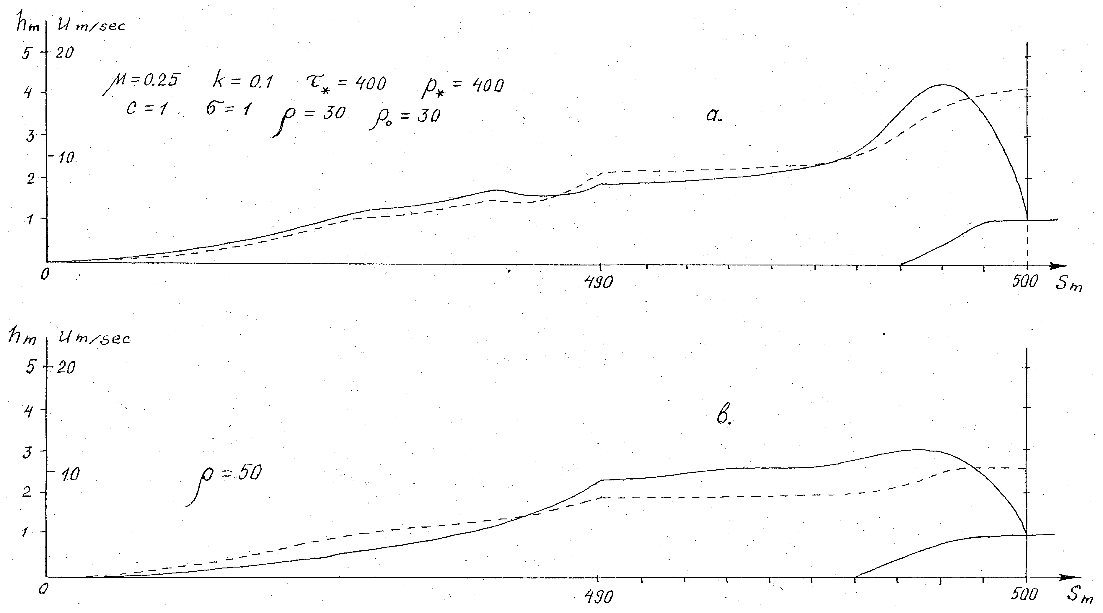
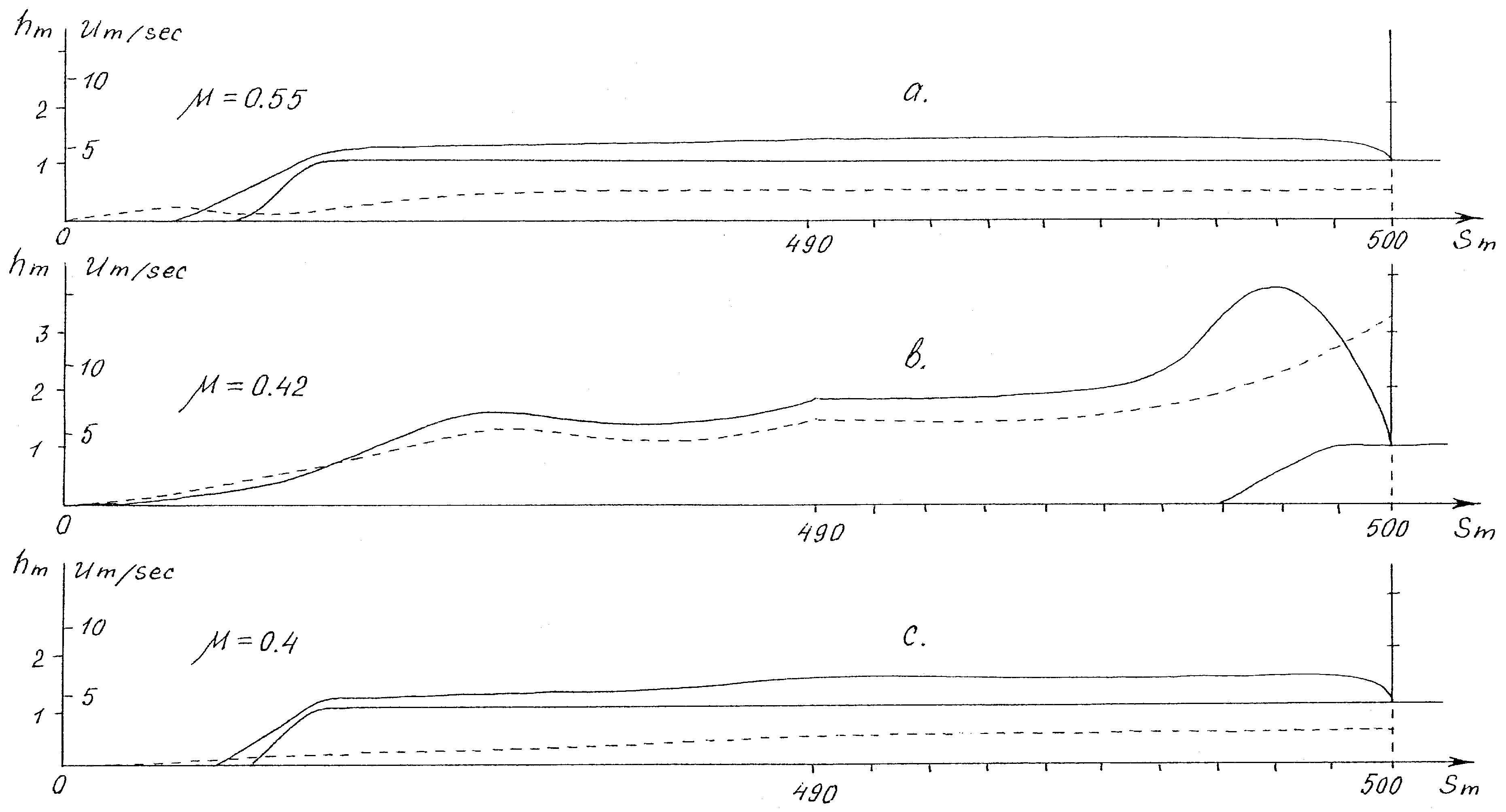
. Except for simulation number 18 (Figure S2.14) with a parabolic, 40 m long and up to 4 m high head followed by a 0.2 m thin tail, the avalanches started as 100 m long and 1 m deep slabs. Five selected simulations are presented in Figure 8 and Figure 9 in terms of the distributions of h and u at the instance when the front reaches the point $S=500$ m. Corresponding plots for the other simulations can be found in the Supplementary Materials Document 2, Figures S2.10–S2.14.

Depending on the combination of the values of the governing parameters, the avalanche behaves according to one of two quite different regimes: One is characterized by intense new-snow entrainment in the frontal zone and the formation of a huge avalanche head. In the other regime, the avalanche is unable to maintain new-snow erosion even if erosion had occurred in the starting zone, resulting in a “weak” avalanche with a spreading body and decreasing velocity. It is very important to note that the governing parameters ($\mu$, k, etc.) determine in a non-monotonic fashion which of these two flow regimes will be realized. As an example, Figure 9 illustrates how, for $0.4\le \mu \le 0.55$, the end values of the range lead to avalanche dynamics of the second, “weak” type, while the intermediate value $\mu =0.42$ is associated with dynamics of the first, “strong” type! ([1], Note 23) This seemingly strange dependence of the mathematical solution of the avalanche dynamics problem is, of course, a consequence of the strong non-linearity of the modified friction law of Grigorian [4]. If the avalanche flow depth is sufficiently small, so that $\tau <{\tau }_{*}$ everywhere and snow accumulation in the avalanche body due to entrainment is weak, then the condition $\tau >{\tau }_{*}$ will never be fulfilled and the avalanche dynamics remains “weak” at all times. If, in contrast, such mass accumulation does occur in some zone (e.g., due to sharp changes in the cross-sectional area of the channel, locally large values of new-snow depth, etc.) and the condition $\tau >{\tau }_{*}$ is met, the avalanche behavior changes in accordance with the friction law, the avalanche “ignites” and becomes highly mobile. As a result, the output parameters characterizing the avalanche motion (mean velocity, thickness, runout distance, etc.) depend on the initial parameters in a stochastic and unpredictable way. From a mathematical point of view, this feature of avalanche dynamics is the most interesting, and it is very important for our general understanding of the avalanche problem.

8. Conclusions

On the one hand, the analytical and computational investigations presented here show that the mathematical problem of quantitative description of snow avalanche dynamics is highly nonlinear and that simple explicit solutions are difficult to obtain. On the other hand, there is a need for simple explicit relations in practical applications. Unfortunately, this need cannot be satisfied to the desired degree for only rough estimations are possible on the basis of very "finite" simplifications made with more or less exact full models. The corresponding procedures are presented and illustrated by numerical calculations in this paper.

One of the most important parameters for practical applications is the maximum runout distance of avalanches at given geographical and climatic conditions. The maximum runout distance corresponds to the most powerful and massive avalanches, in which case one can expect the details of the full model not to be significant. A sufficiently accurate result can in this case presumably be obtained from the simplified model or even from the simplest model described above.

A more difficult problem is quantitative description of the evolving and subsiding avalanche motion, which depends on uncertain information relating to natural data ($\psi \left(S\right)$, $\mu$, $\rho$, ${\tau }_{*}$, etc.), and mathematical modeling of the process of snow entrainment into the avalanche body in the frontal zone. The computational simulation of the avalanche dynamics made with the full model shows that avalanche behavior is stochastic in some sense. Namely, depending on slight differences in the initial data, the bed geometry, etc., mass velocities, depth distribution and other parameters of motion exhibit finite differences and pulsating behavior as the avalanche propagates down the mountain slope. This phenomenon is associated with the dual nature of the assumed bed resistance law: the transitions between the Coulomb law and the ${\tau }_{*}$-law are connected to changes in the flow-depth distribution $H\left(S\right)$, which in turn depends non-linearly on the resistance law. This stochasticity of avalanche dynamics prevents a deterministic description of the full problem; instead, only the statistical characteristics of the main avalanche parameters, as calculated by the (seemingly deterministic) full model, should be evaluated and used in practice.

Nevertheless, there is a program for improving the “exact” full model. It comprises tests of various schemes of snow entrainment at the avalanche front and more adequate modeling of the hydraulic or viscous parts of the resistance, as well as development of a complete software package that integrates all the components of numerical flow simulation and parameter variation that are needed to solve real-world problems. This work remains yet to be done.