Simple Summary
Monitoring animal condition is integral for maintaining a healthy flock, increasing ewe productivity, refining animal nutrition, and identifying suitable animals for slaughter. Accurate determination of the body compositions (the amount of fat, muscle, and bone) of ewes can be used to evaluate their conditions, which provides key information to make management decisions. Farmers currently rely on live weight (LW) and body condition score (BCS) to evaluate the health statuses of ewes. This research proposed the use of visual imaging to determine body dimensions, which are then used in combination with LW to predict the body compositions of ewes. The results showed a correlation between fat, muscle, and bone weight determined by computerized tomography (CT) and the fat, muscle, and bone weight estimated by the live weight and body parameters calculated using the image processing application. The results showed an optimal fat of 9% of LW for ewes during the production cycle. If the percentage of fat is less than or more than 9%, farmers have to take action to improve the conditions of the animals to ensure the best performance during weaning and ewe and lamb survival during the next lambing.
Abstract
Farmers are continually looking for new, reliable, objective, and non-invasive methods for evaluating the conditions of ewes. Live weight (LW) and body condition score (BCS) are used by farmers as a basis to determine the condition of the animal. Body composition is an important aspect of monitoring animal condition. The body composition is the amount of fat, muscle, and bone; knowing the amount of each is important because the information can be used for better strategic management interventions. Experiments were conducted to establish the relationship between body composition and body parameters at key life stages (weaning and pre-mating), using measurements automatically determined by an image processing application for 88 Coopworth ewes. Computerized tomography technology was used to determine the body composition. Multivariate linear regression (MLR), artificial neural network (ANN), and regression tree (RT) statistical analysis methods were used to develop a relationship between the body parameters and the body composition. A subset of data was used to validate the predicted model. The results showed a correlation between fat, muscle, and bone determined by CT and the fat, muscle, and bone weight estimated by the live weight and body parameters calculated using the image processing application, with r2 values of 0.90 for fat, 0.72 for muscle, and 0.50 for bone using ANN. From these results, farmers can utilize these measurements to enhance nutritional and management practices.
1. Introduction
Monitoring and improving individual animal performance is one mechanism to lift economic returns for sheep farming operations [1]. Body condition score (BCS) is a quick and easy way to evaluate ewe condition, using a rating value between one and five; one represents poor, and five represents obese. A ewe in good condition will typically have a BCS between 2.5 and 3.5. BCS is most often defined to the nearest 0.5 increments [2,3,4]. BCS can provide an indication of percentage fat by well-trained evaluators; however, it is a subjective measure [5,6,7,8]. Due to the subjectivity of the BCS, the development of a new scale is required to provide a more accurate estimate of fat [8].
Body composition is the amount of fat, muscle, and bone; knowing the amount of each is important because the information can be used for better farm strategic management interventions [9,10]. It is particularly important to check the ewe’s condition at weaning and pre-mating to ensure the ewe’s condition recovers after weaning, as ewes must be in an optimal condition at pre-mating [11]. These are particularly crucial times in a ewe’s life cycle to make sure it is ready for mating, ensuring ewe and lamb survival in the next lambing, and ensuring the best performance of the animal during weaning [11,12,13,14]. Furthermore, the body composition profiles of ewes between gestation and pre-mating indicate the animals’ reproductive performance [15].
Medical methods such as ultrasound [16,17,18], DEXA [10] and CT [19] are used as research methods for body composition estimation. The accuracy of CT, compared with dissection for determining body composition, achieved r2 values of 0.98 for fat, 0.92 for muscle, and 0.83 for bone [20,21]. However, these methods are time-consuming, expensive, and require expertise, equipment, and special medical procedures [10,18,22].
Body parameters have been used for the determination of yak and ewe LWs using image measurements [23,24,25] and using physical measurements [26,27,28,29]. Body parameters determined by image analysis have been used as a reliable guide for estimating the body size of sheep [30,31,32,33], newborn lamb size [34,35], predicting fat for pigs [36], and carcass characteristics estimation of sheep [37].
Due to BCS subjectivity, the complexity of medical methods and body parameters have not been widely applied to estimate body composition on-farm [38]. Therefore, this paper proposed an alternative method using body parameters determined by an image analysis application coupled with LW to estimate the body compositions of Coopworth ewes and compare this with the BCS, which indicates fat only. To estimate the body composition, three statistical models, MLR, ANN, and RT, were investigated. These models were compared to find the best model between dependent and independent variables in terms of r2 value and error percentage.
2. Materials and Methods
2.1. Experimental Protocol and Approach
Body composition data were determined by CT. LW was measured using a 3-way weigh crate scale manufactured by Prattley. BCS was assessed, and the ewe’s ID was recorded by a farm manager. Ewes were then fixed into a neck brace to take physical body parameters and capture top and side images, and the ewes were then released. Statistical analysis was undertaken to determine which body parameters could predict body composition. Data were collected from 88 ewes aged 2–4 years at Lincoln University farm at weaning and pre-mating. A set of 74 ewes were scanned in both experiments, and 14 ewes were scanned only at weaning. The wool impact factor was determined after the length of the wool was tested and taken into account [39].
2.2. Data Collection
2.2.1. CT Scans
Ewes were CT-scanned at the Lincoln University CT lab using a CT750 HD machine manufactured by GE Healthcare. The CT slice measurements were measured by the CT operator using the STAR 6.15 software.
The animals were fasted with the water removed for 12 h. Lincoln University SOP 83 and Animal Ethical Committee (AEC) #642 approval were followed for the capturing of CT data, LW and physical body measurements, and BCS. Before scanning, the ewes were tranquilized with Acezine 10 mg administered intramuscularly at 0.1 mL/per 10 kg (e.g., a 60 kg ewe was given 0.6 mL, and a 70 kg ewe was given 0.7 mL, and so on) to relax their muscles and keep stress to a minimum. After 20–30 min and once sedated, the ewe was loaded into a wooden CT scanning stretcher in the sternal recumbence position (on its back). Two scout scans were taken, one from the top half of the body and another from the bottom half.
2.2.2. Image Capturing
The ewes were secured in a neck brace, and then top and side images were taken. The neck brace stopped the ewes from moving and helped with keeping them in a standard standing position. Three top images were taken using a GoPro 7 camera (12 Megapixel) mounted orthogonally, with a height of 2350 mm from the ground. The side camera was a Canon DSLR 750D and was used to capture up to three visual side-view images, with 6000 mm between the center of the ewe and the camera and a 760 mm height between the ground and the camera, as shown in Figure 1. The camera had a 24.2 Megapixel CMOS sensor, a DiG!C 6 image processor, and an EF-S 18–135 mm f/3.5–5.6 IS STM lens. While taking the top and side images, two small whiteboards were used to report the animal ID, which was used later during the analysis to identify the animal.
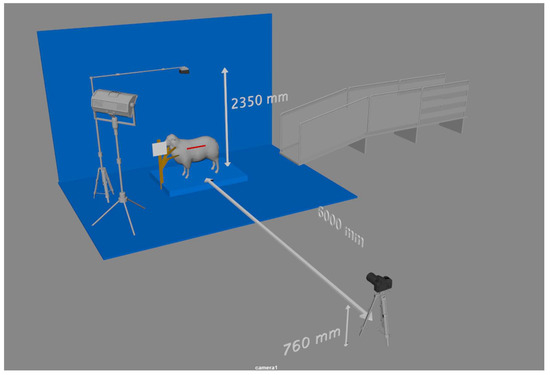
Figure 1.
On-farm weaning and pre-mating experimental setup.
The top body parameters were chest width, width, rump width, top length, and top area (top body area without the head), as shown in Figure 2.
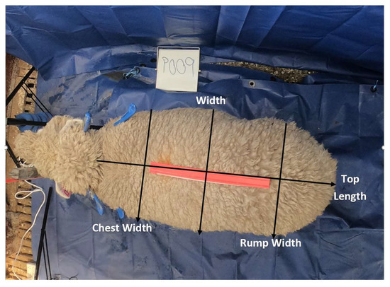
Figure 2.
Ewe top image and body parameters.
The side body parameters were body length from the brisket to the top point of the leg, the side length from the rump dock to the forearm, the angle length from the neck to the top point of the hock, the height from the lowest point of the front hoof to the top shoulder, the depth from the top rack to the lowest point of the belly, and the side area (side body area without head and legs), as shown in Figure 3. Body parameters of width, top length, front height, body length, angle length, depth and side length, chest width, rump width, back height, top, and side areas were determined by an image-processing application at weaning and using pre-mating scans. This application was developed using image-processing functions from the OpenCV library. Once an image is uploaded to the application, it will determine body parameters. These body parameters with LW are then used in the application to estimate the body composition using the prediction models.
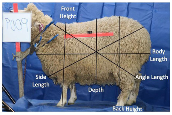
Figure 3.
Ewe side image and body parameters.
2.3. Statistical Analysis
The data from the weaning and premating experiments were combined, yielding 162 observations. A set of 138 observations were used as training data, and the remaining 24 observations were used as testing data. For ANN, 114 observations were used as the training set, 24 observations were used as a validation set, and the remaining 24 observations were used as a testing set. Factor analysis was used to check the correlation between the body parameters of the training data.
3. Results
3.1. Descriptive Statistics
The descriptive statistics were presented for the training data. The descriptive analysis showed the minimum, maximum, mean, and standard deviations of all ewes, as shown in Table 1. The amount of fat had a wider range, compared with muscle and bone. The minimum fat amount determined was 0.88 kg, compared to a maximum of 17.64 kg, while the minimum bone amount determined was 2.03 kg, and the maximum was 3.77 kg.

Table 1.
Descriptive statistics of the training data.
Ewes that had a BCS between 2.5–3.5 had a minimum fat = 1.29 kg and a maximum fat = 13.86 kg, with an average fat = 5.55 kg. Within this BCS range, ewes had a minimum LW = 47.5 kg and a maximum LW = 78.5 kg, with an average LW = 59.2 kg. Then, based on the average BCS and average LW, an optimal fat amount for ewes was found to be around 9% of the LW.
3.2. Application Accuracy
The results showed an average absolute difference of 4% for body parameters measured by the custom ruler and body parameters determined by the image-processing application, as shown in Table 2. The impact of wool length on the body parameters was tested on five ewes to find the adjustment amount. After adjustment, all parameters decreased slightly, and LW decreased by 1200 g.
Table 2.
Average error % of absolute weaning and pre-mating between actual and app measurements.
3.3. Factor Analysis
The collinearity check in Table 3 shows the collinearity between independent variables based on three components, where each component had variables that had high collinearity between them. The first component included chest width, angle length, body length, side length, top length, width, rump width, top area, and side area. The second component included the BCS and LW. The third component included height and back height.
Table 3.
Rotated component matrix.
3.4. Fat
After testing all possible combinations of the independent variables for the estimation of fat based on factor analysis, as shown in Table 4, a relationship between the independent variables’ weights and chest widths with the dependent variable fat was established. The final multivariate regression model estimated the fat to have an r2 = 0.79 and an RMSE = 1.34, with no co-linearity obtained. The result was tested using 24 ewes and showed that r2 = 0.87, and RMSE = 1.40.
Table 4.
Relationships between LW and body parameters to estimate fat—MLR.
For ANN, the predicted model accounted for fat, with an r2 = 0.88 and an RMSE = 1.17 for the training data. This model had two inputs—LW and chest width—with one hidden layer and one output (fat), with no collinearity. However, all variable models were examined to show the possible maximum result, with an r2 = 0.95 and RMSE = 1.22, as shown in Table 5. The known amount of fat was tested, and a relationship was found to validate the fat prediction model using the test data, with an r2 = 0.94 and an RMSE = 1.01.
Table 5.
Relationships between LW and body parameters to estimate fat—ANN.
For the regression tree, different combinations between body parameters were analyzed and compared. The model with the highest r2 value and lowest RMSE for the prediction of fat used two variables: LW and chest width, with r2 = 0.67 and RMSE = 1.75. The model was validated, and the result showed that r2 = 0.72, and RMSE = 1.42.
3.5. Muscle
The highest r2 to estimate muscle was found between the LW and width model. The model was statistically significant (p-values ≤ 0.05), with r2 = 0.52 and RMSE = 1.03, with no co-linearity obtained, and the equation is displayed in Table 6. The results for the test data showed an r2 = 0.41 and an RMSE = 0.86 between the actual and predicted muscles.
Table 6.
Relationships between LW and body parameters to estimate muscle—MLR.
One model was selected for muscle prediction, with r2 = 0.77 and RMSE = 1.26, using ANN with one hidden layer used and three inputs (LW, rump width, front height). The highest predicted model accounted for muscle, with r2 = 0.79 and RMSE = 1.20 for using all variables and r2 = 0.72 and RMSE = 1.03 for test data, as shown in Table 7.
Table 7.
Relationships between LW and body parameters to estimate muscle—ANN.
The regression tree model for the prediction of muscle from independent variables used LW, width, and chest width. The results showed that muscle had an r2 = 0.25 and an RMSE = 1.27 for training data and an r2 = 0.21 and an RMSE = 1.19 for test data.
3.6. Bone
The highest r2 was found for the relationship using all of the variables, but this relationship was rejected, as it was against the factor analysis. The next highest r2 value to estimate bone was found for the relationship between LW and width, with an r2 = 0.26 and an RMSE = 0.87, as shown in Table 8.
Table 8.
Relationships between LW and body parameters to estimate bone—MLR.
The results of the test data showed an r2 of 0.34 and an RMSE = 0.26 between the CT bone and the predicted bone. It was noticed that the bone had a very small variation between 2.03 kg and 3.77 kg, which could explain the low r2 value, as mentioned in descriptive statistics.
All combinations of the independent variables were compared according to the highest r2 value and the lowest RMSE. A relationship of r2 = 0.75 with an RMSE = 2.40 to estimate bone was found using all variables. However, one model had three inputs: LW and width, front height, and one hidden layer. The predicted model accounted for bone, with r2 = 0.72 and RMSE = 1.11, as shown in Table 9. The model was tested and showed an r2 = 0.50 and an RMSE = 1.21.
Table 9.
Relationships between LW and body parameters to estimate bone—ANN.
The model with LW, rump width, and chest width was the model used to estimate the amount of bone, with r2 = 0.05 and RMSE = 0.30 using regression tree. The best model for bone estimation was tested, and the result showed that r2 = 0.03, and RMSE = 0.70.
3.7. Summary of Results
All statistical method results were compared in terms of r2 and RMSE using 24 ewes at the same points of the breeding cycle, as shown in Table 10. For test data, ANN matrixes were produced to estimate dependent variables. The ANN showed the highest results for test data for fat with an r2 = 0.90 and an RMSE = 1.01; for muscle with an r2 = 0.72 and an RMSE = 1.03; and for bone with an r2 = 0.50 and an RMSE = 1.21.
Table 10.
Test data prediction of 24 ewes—ANN vs. MLR vs. RT.
The ANN matrixes were then used in the image-processing application to calculate body composition, as shown in Figure 4.
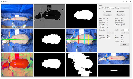
Figure 4.
Output screen of the image-processing application.
In summary, ANN models were the best in terms of the highest r2 values and lowest RMSEs for the prediction of fat, muscle, and bone, compared with MLR and RT. ANN matrixes were produced to estimate body composition using input variables.
The results of fat estimation for the test data between the ANN, MLR, and RT, along with BCS results, are shown in Table 11. The maximum difference for the MLR, compared with CT fat, was 3.1 kg, and there was a minimum difference of 0.002 kg. For ANN, there was a 2.69 kg maximum difference and a 0.034 kg minimum difference. The RT had a maximum difference of 8.34 kg and a minimum difference of 0.59 kg.
Table 11.
Fat test data estimation in (kg)—body condition score.
The BCS result showed a range of fat estimation between 3.52–13.03 kg for condition 2.5 and a range of 5.11–13.86 kg for a score of 3.0. Two ewes had fat amounts of 5.14 kg and 7.91 kg with condition 3.5, and another ewe had a fat amount of 4.39 kg with a condition score of 4.0. The CT fat and ANN fat results based on BCS are shown in Figure 5.
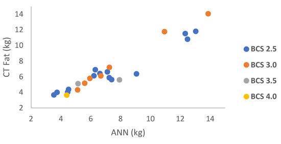
Figure 5.
Relationship between CT fat vs. ANN fat based on BCS.
4. Discussion
An alternative method to predict the body composition of ewes during their production life cycle was proposed. The farmer first weighed the sheep, then took top and side images using fixed-top and side cameras where the sheep was constrained. The farmer then input the data (images and LW) to the computer, where the application was installed. The application then displayed the amount of fat, muscle, and bone. For example, if the amount of fat was less than or more than 9% of the LW, then the farmer had to evaluate the status of energy reserves and provide the required nutritional intake [40]. The setup of the new method required using top and side cameras, an electronic scale, and a little training. This allowed farmers to have their setup and use this method at any time without moving ewes away from the farm or exposing animals to machine radiation while scanning. The new method required less effort and time and did not need technical expertise and tranquillization of sheep with Acezine the way the CT method does [20]. The CT method had high r2 values of 0.98 for fat, 0.92 for muscle, and 0.83 for bone, whereas the new method showed lower r2 values of 0.90 for fat, 0.72 for muscle, and 0.50 for bone. Body fat was predicted on-farm by subjective methods, such as BCS [8]. A BCS between 2.5–3.5 meant a ewe was in good condition [2]. The development of a new BCS scale was required to provide a more accurate estimation of the fat of ewes [8]. BCS can provide a good indication of fat percentage, as stated by Tait et al. [5]. In contrast, the results of this study showed a range of fat between 1.29 kg and 13.86 kg, with an average fat of 5.55 kg for a BCS between 2.5 and 3.5. A narrower range or percentage is needed for farmers to evaluate the health of their livestock because this range is too vast. This study’s findings revealed that 9% of fat to the LW was ideal for ewes. The results showed that many ewes had the same BCS, which provided a rough indication of ewe condition, but there was a wide range of chest widths and fat measurements, confirming that the BCS was not just subjective but also inaccurate for evaluating fat. For example, one ewe had 5.2 kg of fat, a BCS of 3.0, and a chest width of 252 mm at weaning, then 7.1 kg fat, 3.0 BCS, and a chest width of 327.6 mm at pre-mating. This shows that fat and chest width increased over time, but the BCS remained the same. This is in line with other studies that showed a high variation of fat within certain BCSs [4,8]. This research used measurements such as LW and chest width, width, rump width, and front height. In the results, fat was predicted with an r2 = 0.90, which was higher than the study by Doeschl et al. [36], which had an r2 = 0.69 using rump width only, which explains that using LW will increase the accuracy. The majority of previous studies used linear methods such as MLR to predict body composition. This research used the linear method (MLR) [18,21,36,37] and non-linear methods (ANN, RT) to predict body composition and made a comparison between them. The ANN method showed the highest r2 values and the lowest RMSE.
5. Conclusions
The body composition of ewes can now be determined using a new technique that was developed using an image-processing application. Instead of relying on a wide range of BCSs between 2.5–3.5, this technique aids farmers in making decisions if the amount of fat is less than or more than 9% of the LW. The technique can be used to measure body parameter values on shorn or woolly ewes. The suggested method yields less subjective results than the BCS. This method is based on predicting body composition at two different points in the production cycle. Farmers can use the application with little training provided. Farmers can also use the equations of MLR to estimate fat with an r2 that reaches 0.87.
Author Contributions
A.S. led the conception and design of the research. Material preparation, analysis and results were carried out by A.S. Data collection was undertaken by A.S. and C.L., and they were assisted by S.P., P.A., S.C. and M.S. The first draft of the manuscript was written by A.S. All authors have read and agreed to the published version of the manuscript.
Funding
This research received no external funding.
Institutional Review Board Statement
The animal study protocol was approved by Lincoln University SOP 83 and Animal Ethical Committee (AEC) #642—AEC 2020-19 on 22 July 2020.
Informed Consent Statement
Not applicable.
Data Availability Statement
The data presented in this study are available upon request from the corresponding author.
Conflicts of Interest
The authors declare no conflict of interest.
References
- Silva, S.; Cadavez, V. Real-time ultrasound (RTU) imaging methods for quality control of meats. In Computer Vision Technology in the Food and Beverage Industries; Woodhead Publishing: Sawston, UK, 2012; pp. 277–329. [Google Scholar]
- Keinprecht, H.; Pichler, M.; Pothmann, H.; Huber, J.; Iwersen, M.; Drillich, M. Short term repeatability of body fat thickness measurement and body condition scoring in sheep as assessed by a relatively small number of assessors. Small Rumin. Res. 2016, 139, 30–38. [Google Scholar] [CrossRef]
- Kenyon, P.R.; Maloney, S.K.; Blache, D. Review of sheep body condition score in relation to production characteristics. N. Z. J. Agric. Res. 2014, 57, 38–64. [Google Scholar] [CrossRef]
- Russel, A. Body condition scoring of sheep. Practice 1984, 6, 91. [Google Scholar] [CrossRef]
- Tait, I.M.; Kenyon, P.R.; Garrick, D.J.; Lopez-Villalobos, N.; Pleasants, A.B.; Hickson, R.E. Associations of body condition score and change in body condition score with lamb production in New Zealand Romney ewes. N. Z. J. Anim. Sci. Prod. 2019, 79, 91–94. [Google Scholar]
- Van Burgel, A.J.; Oldham, C.M.; Behrendt, R.; Curnow, M.; Gordon, D.J.; Thompson, A.N. The merit of condition score and fat score as alternatives to liveweight for managing the nutrition of ewes. Anim. Prod. Sci. 2011, 51, 834–841. [Google Scholar] [CrossRef]
- McHugh, N.; McGovern, F.; Creighton, P.; Pabiou, T.; McDermott, K.; Wall, E.; Berry, D.P. Mean difference in live-weight per incremental difference in body condition score estimated in multiple sheep breeds and crossbreds. Animal 2019, 13, 549–553. [Google Scholar] [CrossRef] [PubMed]
- Termatzidou, S.A.; Siachos, N.; Valergakis, G.E.; Georgakopoulos, A.; Patsikas, M.N.; Arsenos, G. Association of body condition score with ultrasound backfat and longissimus dorsi muscle depth in different breeds of dairy sheep. Livest. Sci. 2020, 236, 104019. [Google Scholar] [CrossRef]
- Moro, A.B.; Pires, C.C.; da Silva, L.P.; Menegon, A.M.; Venturini, R.S.; Martins, A.A.; Galvani, D.B. Prediction of physical characteristics of the lamb carcass using in vivo bioimpedance analysis. Animal 2019, 13, 1744–1749. [Google Scholar] [CrossRef]
- Miller, D.; Ellen, J.B.; Joanne, L.H.; Fiona, A.; Clare, L.A. Dual-energy X-ray absorptiometry scans accurately predict differing body fat content in live sheep. J. Anim. Sci. Biotechnol. 2019, 10, 248–253. [Google Scholar] [CrossRef]
- Cam, M.A.; Garipoglu, A.V.; Koray, K. Body condition status at mating affects gestation length, offspring yield and return rate in ewes. Arch. Für Tierz. 2018, 61, 221–228. [Google Scholar] [CrossRef]
- MacLaughlin, S.M.; Walker, S.K.; Roberts, C.T.; Kleemann, D.O.; McMillen, I.C. Periconceptional nutrition and the relationship between maternal body weight changes in the periconceptional period and feto-placental growth in the sheep. J. Physiol. 2005, 565, 111–124. [Google Scholar] [CrossRef] [PubMed]
- Borg, R.C.; Notter, D.R.; Kott, R.W. Phenotypic and genetic associations between lamb growth traits and adult ewe body weights in western range sheep. J. Anim. Sci. 2009, 87, 3506–3514. [Google Scholar] [CrossRef] [PubMed]
- Fthenakis, G.C.; Mavrogianni, V.S.; Gallidis, E.; Papadopoulos, E. Interactions between parasitic infections and reproductive efficiency in sheep. Vet. Parasitol. 2015, 208, 56–66. [Google Scholar] [CrossRef] [PubMed]
- Manly, H.; Shackell, G.; Greer, G.J.; Everett-Hincks, J. The association of ewe body condition with weight of lamb weaned. Proc. N. Z. Soc. Anim. Prod. 2011, 71, 62–65. [Google Scholar]
- Ribeiro, F.; Thompson, A.; Aragon, S.; Hosford, A.; Hergenreder, J.; Jennings, M.; Johnson, B. Comparison of real-time ultrasound measurements for body composition traits to carcass and camera data in feedlot steers. Prof. Anim. Sci. 2014, 30, 597–601. [Google Scholar] [CrossRef]
- Dias, L.; Silva, S.; Teixeira, A. Simultaneously prediction of sheep and goat carcass composition and body fat depots using in vivo ultrasound measurements and live weight. Res. Vet. Sci. 2020, 133, 180–187. [Google Scholar] [CrossRef]
- Morales-Martinez, M.A.; Arce-Recinos, C.; Mendoza-Taco, M.M.; Luna-Palomera, C.; Ramirez-Bautista, M.A.; Piñeiro-Vazquez, Á.T.; Vicente-Perez, R.; Tedeschi, L.O.; Chay-Canul, A.J. Developing equations for predicting internal body fat in Pelibuey sheep using ultrasound measurements. Small Rumin. Res. 2020, 183, 106031. [Google Scholar] [CrossRef]
- Kvame, T.; Vangen, O. Selection for lean weight based on ultrasound and CT in a meat line of sheep. Livest. Sci. 2007, 106, 232–242. [Google Scholar] [CrossRef]
- Macfarlane, J.M.; Lewis, R.M.; Emmans, G.C.; Young, M.J.; Simm, G. Predicting carcass composition of terminal sire sheep using X-ray computed tomography. Anim. Sci. 2007, 82, 289–300. [Google Scholar] [CrossRef]
- Johnson, P.; Juengel, J.; Bain, W. Predicting internal adipose from selected computed tomography images in sheep. N. Z. J. Anim. Sci. Prod. 2020, 80, 113–116. [Google Scholar]
- Bain, W.; Hickey, S.; Clarke, S.; McEwan, J. Estimation of Computed Tomography (CT) Predicted Meat Yield in New Zealand Lamb. In Proceedings of the 11th World Congress on Genetics Applied to Livestock Production, Auckland, New Zealand, 11–16 February 2018. [Google Scholar]
- Riva, J.; Rizzi, R.; Marelli, S.; Cavalchini, L.G. Body measurements in Bergamasca sheep. Small Rumin. Res. 2004, 55, 221–227. [Google Scholar] [CrossRef]
- Yan, Q.; Ding, L.; Wei, H.; Wang, X.; Jiang, C.; Degen, A. Body weight estimation of yaks using body measurements from image analysis. Measurement 2019, 140, 76–80. [Google Scholar] [CrossRef]
- Zhang, Y.; Sun, Z.; Zhang, C.; Yin, S.; Wang, W.; Song, R. Body Weight Estimation of Yak Based on Cloud Edge Computing. EURASIP J. Wirel. Commun. Netw. 2021, 1–20. [Google Scholar] [CrossRef]
- Yilmaz, O.; Cemal, I.; Karaca, O. Estimation of mature live weight using some body measurements in Karya sheep. Trop. Anim. Health Prod. 2013, 45, 397–403. [Google Scholar] [CrossRef]
- Topai, M.; Macit, M. Prediction of Body Weight from Body Measurements in Morkaraman Sheep. J. Appl. Anim. Res. 2004, 25, 97–100. [Google Scholar] [CrossRef]
- Iqbal, F.; Ali, M.; Huma, Z.; Raziq, A. Predicting Live Body Weight Of Harnai Sheep Through Penalized Regression Models. J. Anim. Plant Sci. 2019, 29, 1541–1548. [Google Scholar]
- Sabbioni, A.; Beretti, V.; Superchi, P.; Ablondi, M. Body weight estimation from body measures in Cornigliese sheep breed. Ital. J. Anim. Sci. 2020, 19, 25–30. [Google Scholar] [CrossRef]
- Burke, J.; Nuthall, P.L.; McKinnon, A.E. An Analysis of the Feasibility Of Using Image Processing To Estimate the Live Weight of Sheep; Farm Hortic. Farm and Horticultural Management Group Applied Management and Computing Division Lincoln University: Canterbury, New Zealand, 2004. [Google Scholar]
- Zhang, A.L.N.; Wu, B.P.; Jiang, C.X.H.; Xuan, D.C.Z.; Ma, E.Y.H.; Zhang, F.Y.A. Development and validation of a visual image analysis for monitoring the body size of sheep. J. Appl. Anim. Res. 2018, 46, 1004–1015. [Google Scholar] [CrossRef]
- Abdelhady, A.; Hassanien, A.E.; Awad, Y.; El-Gayar, M.; Fahmy, A. Automatic Sheep Weight Estimation Based on K-Means Clustering and Multiple Linear Regression. In Proceedings of the International Conference on Advanced Intelligent Systems and Informatics 2018; Springer International: Manila, Philippines, 2019; pp. 546–555. [Google Scholar]
- Zhang, A.; Wu, B.; Wuyun, C.; Jiang, D.; Xuan, E.; Ma, F. Algorithm of sheep body dimension measurement and its applications based on image analysis. Comput. Electron. Agric. 2018, 153, 33–45. [Google Scholar] [CrossRef]
- Puth, M.-T.; Neuhäuser, M.; Ruxton, G.D. Effective use of Spearman’s and Kendall’s correlation coefficients for association between two measured traits. Anim. Behav. 2015, 102, 77–84. [Google Scholar] [CrossRef]
- Khojastehkey, M.; Aslaminejad, A.A.; Shariati, M.M.; Dianat, R. Body size estimation of new born lambs using image processing and its effect on the genetic gain of a simulated population. J. Appl. Anim. Res. 2016, 44, 326–330. [Google Scholar] [CrossRef]
- Doeschl, A.B.; Green, D.M.; Whittemore, C.T.; Schofield, C.P.; Fisher, A.V.; Knap, P.W. The relationship between the body shape of living pigs and their carcass morphology and composition. Anim. Sci. 2004, 79, 73–83. [Google Scholar] [CrossRef]
- Bautista-Díaz, E.; Mezo-Solis, J.A.; Herrera-Camacho, J.; Cruz-Hernández, A.; Gomez-Vazquez, A.; Tedeschi, L.O.; Lee-Rangel, H.A.; Vargas-Bello-Pérez, E.; Chay-Canul, A.J. Prediction of Carcass Traits of Hair Sheep Lambs Using Body Measurements. Animals 2020, 10, 1276. [Google Scholar] [CrossRef] [PubMed]
- Lonergan, S.M.; Topel, D.G.; Marple, D.N. Chapter 8–Methods to measure body composition of domestic animals. In The Science of Animal Growth and Meat Technology, 2nd ed.; Lonergan, S.M., Topel, D.G., Marple, D.N., Eds.; Academic Press: Cambridge, MA, USA, 2019; pp. 125–146. [Google Scholar]
- Cottle, D. International Sheep and Wool Handbook, 1st ed.; Nottingham University Press: Nottingham, UK, 2010; p. 766. [Google Scholar]
- Maeno, H.; Oishi, K.; Hirooka, H. Interspecies differences in the empty body chemical composition of domestic animals. Animal 2013, 7, 1148–1157. [Google Scholar] [CrossRef] [PubMed]
Disclaimer/Publisher’s Note: The statements, opinions and data contained in all publications are solely those of the individual author(s) and contributor(s) and not of MDPI and/or the editor(s). MDPI and/or the editor(s) disclaim responsibility for any injury to people or property resulting from any ideas, methods, instructions or products referred to in the content. |
© 2023 by the authors. Licensee MDPI, Basel, Switzerland. This article is an open access article distributed under the terms and conditions of the Creative Commons Attribution (CC BY) license (https://creativecommons.org/licenses/by/4.0/).