GPS Tracking to Monitor the Spatiotemporal Dynamics of Cattle Behavior and Their Relationship with Feces Distribution


Abstract
:Simple Summary
Abstract
1. Introduction
2. Materials and Methods
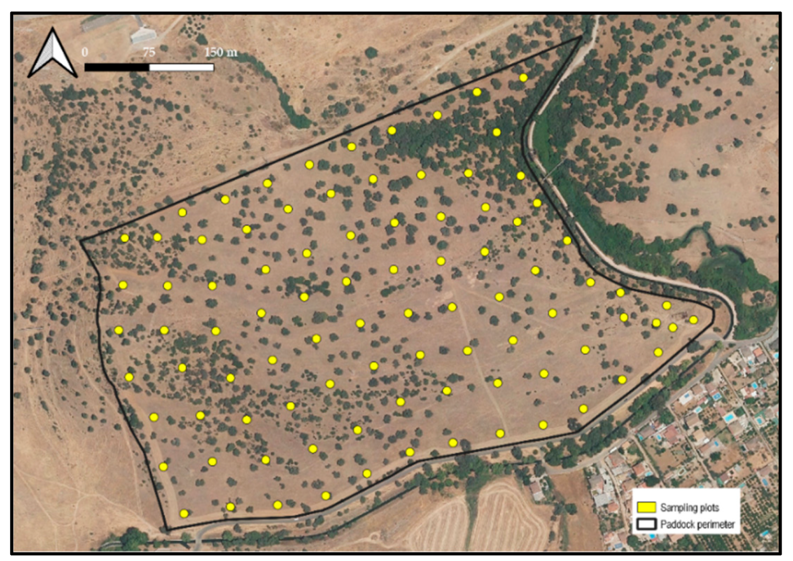
2.1. Study Area
2.2. Cattle Monitoring
2.3. Characterization of Dung Distribution
2.4. Characterization of Factors Affecting the Spatial Variability of Grazing Behavior
2.5. Characterization of Factors Affecting the Temporal Variability of Grazing Behavior
2.6. Data Processing and Analysis
3. Results
3.1. Effects of Spatial Patterns on Cattle and Dung Distribution
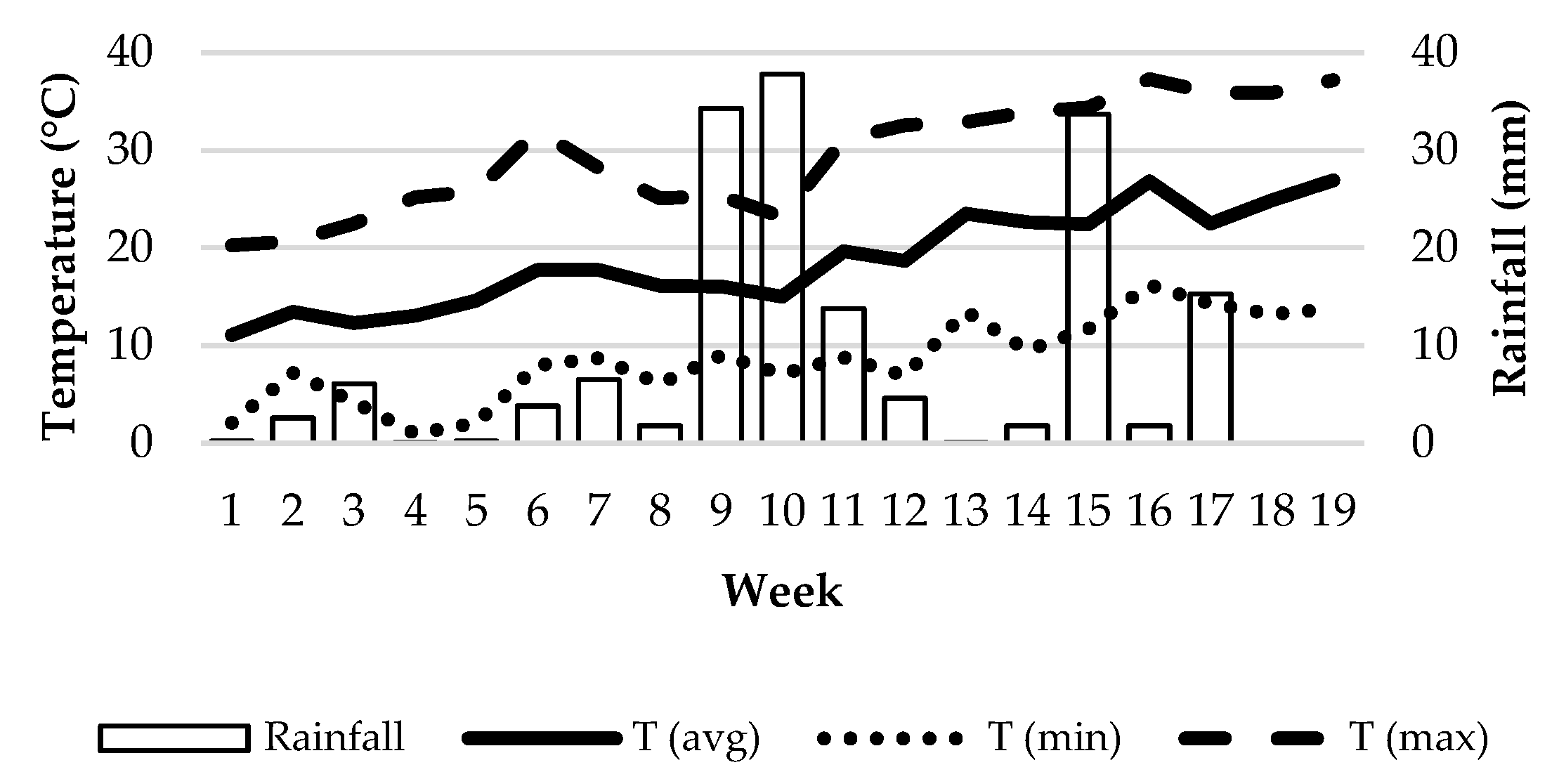
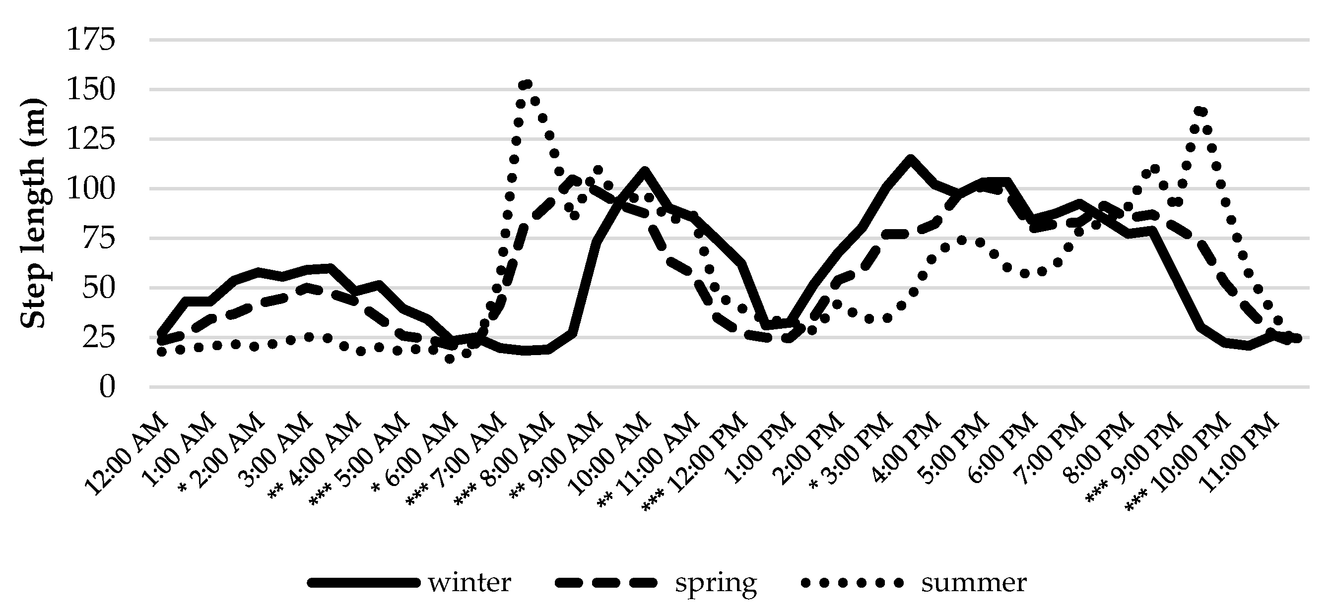
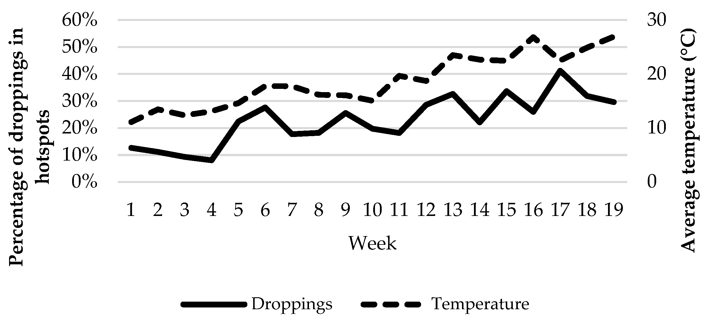
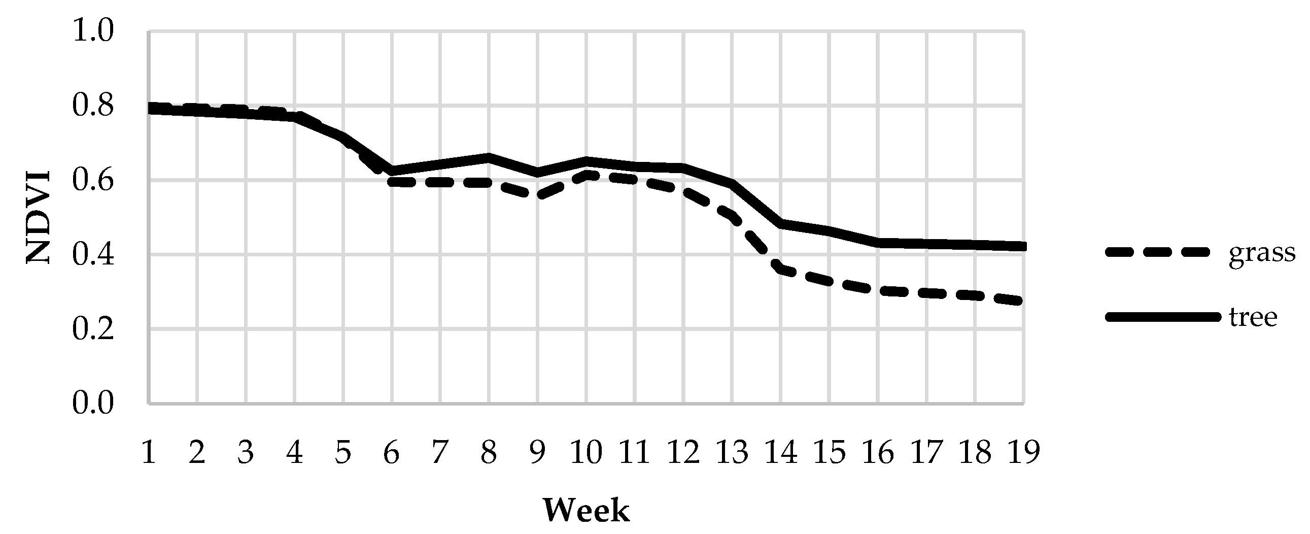
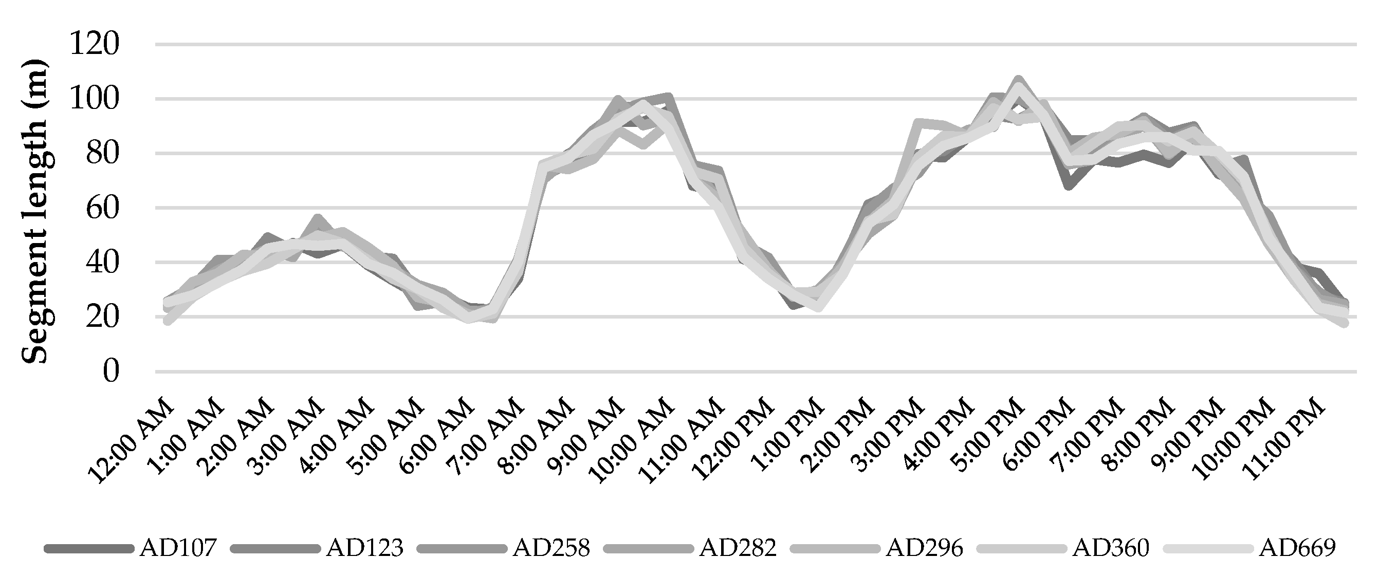
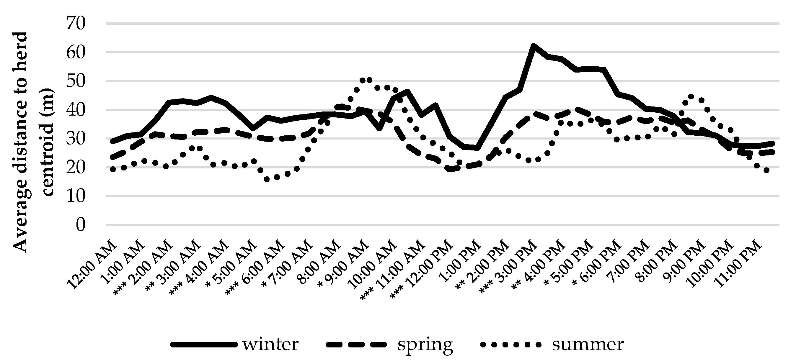
3.2. Effects of Temporal Patterns on Cattle and Dung Distribution
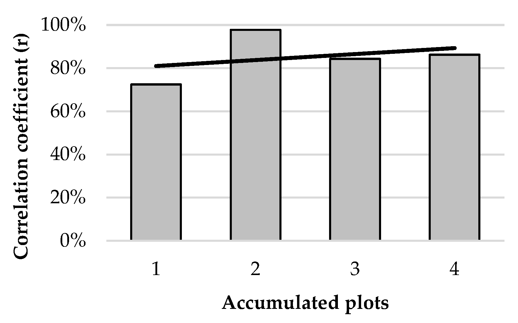
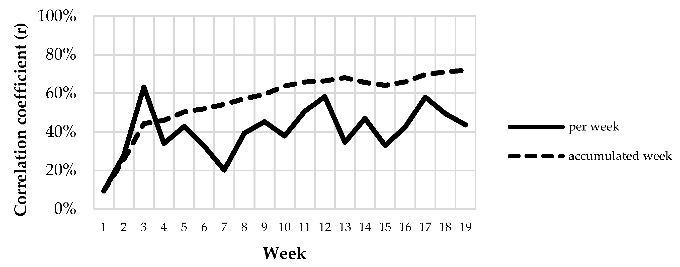
3.3. Relationships between GPS Data and Dung Accumulation in Sampling Plots
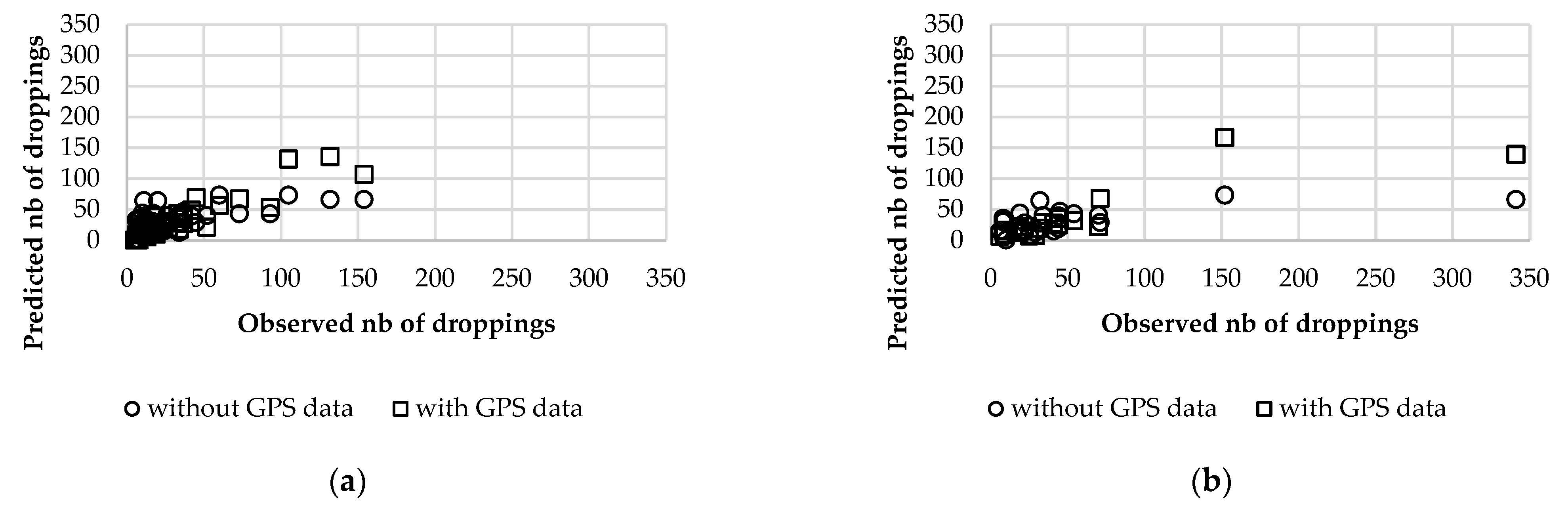
3.4. Calibration and Validation of Prediction Models
4. Discussion
5. Conclusions
Supplementary Materials
Author Contributions
Funding
Institutional Review Board Statement
Informed Consent Statement
Data Availability Statement
Acknowledgments
Conflicts of Interest
References
- Sharrow, S.H.; Brauer, D.; Clason, T.R. Silvopastoral Practices. In North American Agroforestry: An Integrated Science and Practice, 2nd ed.; Garrett, H.E.G., Ed.; Wiley: New York, NY, USA, 2009; pp. 105–131. [Google Scholar] [CrossRef]
- Carpinelli, S.; da Fonseca, A.F.; Weirich Neto, P.H.; Dias, S.H.; Pontes, L.D. Spatial and Temporal Distribution of Cattle Dung and Nutrient Cycling in Integrated Crop-Livestock Systems. Agronomy 2020, 10, 672. [Google Scholar] [CrossRef]
- Garrett, H.E.; Buck, L. Agroforestry practice and policy in the United States of America. For. Ecol. Manag. 1997, 91, 5–15. [Google Scholar] [CrossRef]
- Díaz, M.; Pulido, F. Dehesas Perennifolias de Quercus spp. Bases Ecológicas Preliminares para la Conservación de los Tipos de Hábitat de Interés Comunitario en España; Ministerio de Medio Ambiente, y Medio Rural y Marino: Madrid, Spain, 2009; 69p. [Google Scholar]
- Martínez-Ruedas, C.; Guerrero-Ginel, J.E.; Fernández-Ahumada, E. A Methodology for Automatic Identification of Units with Ecological Significance in Dehesa Ecosystems. Forests 2022, 13, 581. [Google Scholar] [CrossRef]
- White, S.; Sheffield, R.; Washburn, S.; King, L.; Green, J. Spatial and Time Distribution of Dairy Cattle Excreta in an Intensive Pasture System. J. Environ. Qual. 2001, 30, 2180–2187. [Google Scholar] [CrossRef] [PubMed]
- Draganova, I.; Yule, I.; Stevenson, M.; Betteridge, K. The effects of temporal and environmental factors on the urination behaviour of dairy cows using tracking and sensor technologies. Precis. Agric. 2016, 17, 407–420. [Google Scholar] [CrossRef]
- Koch, B.; Homburger, H.; Edwards, P.J.; Schneider, M.K. Phosphorus redistribution by dairy cattle on a heterogeneous subalpine pasture, quantified using GPS tracking. Agric. Ecosyst. Environ. 2018, 257, 183–192. [Google Scholar] [CrossRef]
- Sanderson, M.A.; Feldmann, C.; Schmidt, J.; Herrmann, A.; Taube, F. Spatial distribution of livestock concentration areas and soil nutrients in pastures. J. Soil Water Conserv. 2010, 65, 180. [Google Scholar] [CrossRef]
- Oudshoorn, F.W.; Kristensen, T.; Nadimi, E.S. Dairy cow defecation and urination frequency and spatial distribution in relation to time-limited grazing. Livest. Sci. 2008, 113, 62–73. [Google Scholar] [CrossRef]
- Fan, J.; Jin, H.; Zhang, C.; Zheng, J.; Zhang, J.; Han, G. Grazing intensity induced alternations of soil microbial community composition in aggregates drive soil organic carbon turnover in a desert steppe. Agric. Ecosyst. Environ. 2021, 313, 107387. [Google Scholar] [CrossRef]
- Trotter, M.G.; Lamb, D.W.; Hinch, G.N.; Guppy, C.N. GNSS Tracking of livestock: Towards variable fertilizer strategies for the grazing industry. In Proceedings of the 10th International Conference on Precision Agriculture, Denver, CO, USA, 18–21 July 2010; pp. 18–20. [Google Scholar]
- McGechan, M.B.; Topp, C.F.E. Modelling environmental impacts of deposition of excreted nitrogen by grazing dairy cows. Agric. Ecosyst. Environ. 2004, 103, 149–164. [Google Scholar] [CrossRef]
- Eriksen, J.; Kristensen, K. Nutrient excretion by outdoor pigs: A case study of distribution, utilization and potential for environmental impact. Soil Use Manag. 2001, 17, 21–29. [Google Scholar] [CrossRef]
- Franzluebbers, A.J.; Stuedemann, J.A.; Schomberg, H.H. Spatial Distribution of Soil Carbon and Nitrogen Pools under Grazed Tall Fescue. Soil Sci. Soc. Am. J. 2000, 64, 635–639. [Google Scholar] [CrossRef]
- Schnyder, H.; Locher, F.; Auerswald, K. Nutrient redistribution by grazing cattle drives patterns of topsoil N and P stocks in a low-input pasture ecosystem. Nutr. Cycl. Agroecosystems 2010, 88, 183–195. [Google Scholar] [CrossRef]
- Lan, L.; Zhang, J.; He, X.; Hou, F. Different effects of sheep excrement type and supply level on plant and soil C: N: P stoichiometry in a typical steppe on the loess plateau. Plant Soil 2021, 462, 45–58. [Google Scholar] [CrossRef]
- Tate, K.W.; Atwill, E.R.; McDougald, N.K.; George, M.R. Spatial and temporal patterns of cattle feces deposition on rangeland. J. Range Manag. 2003, 56, 432–438. [Google Scholar] [CrossRef]
- Islam, T.; Fukuda, E.; Shiyomi, M.; Shaibur, M.R.; Kawai, S.; Tsuiki, M. Effects of Feces on Spatial Distribution Patterns of Grazed Grassland Communities. Agric. Sci. China 2010, 9, 121–129. [Google Scholar] [CrossRef]
- Yamada, D.; Higashiyama, M.; Yamaguchi, M.; Shibuya, T.; Shindo, K.; Tejima, S. Spatial Distribution of Cattle Dung Excretion and Dung Nutrients on a Sloping Pasture. Jpn. J. Grassl. Sci. 2011, 57, 129–135. [Google Scholar] [CrossRef]
- Marion, G.; Smith, L.A.; Swain, D.L.; Davidson, R.S.; Hutchings, M.R. Agent-based modelling of foraging behaviour: The impact of spatial heterogeneity on disease risks from faeces in grazing systems. J. Agric. Sci. 2008, 146, 507–520. [Google Scholar] [CrossRef]
- Zhang, L.; Kim, J.; Lee, Y. The platform development of a real-time momentum data collection system for livestock in wide grazing land. Electronics 2018, 7, 71. [Google Scholar] [CrossRef] [Green Version]
- Kemp, D.R.; Michalk, D.L. Towards sustainable grassland and livestock management. J. Agric. Sci. 2007, 145, 543–564. [Google Scholar] [CrossRef]
- Odintsov Vaintrub, M.; Levit, H.; Chincarini, M.; Fusaro, I.; Giammarco, M.; Vignola, G. Review: Precision livestock farming, automats and new technologies: Possible applications in extensive dairy sheep farming. Animal 2021, 15, 100143. [Google Scholar] [CrossRef] [PubMed]
- Monteiro, A.; Santos, S.; Gonçalves, P. Precision Agriculture for Crop and Livestock Farming-Brief Review. Animals 2021, 11, 2345. [Google Scholar] [CrossRef] [PubMed]
- Laca, E. Precision livestock production: Tools and concepts. R. Bras. Zootec. 2009, 38, 123–132. [Google Scholar] [CrossRef]
- Rivero, M.J.; Grau-Campanario, P.; Mullan, S.; Held, S.; Stokes, J.; Lee, M.; Cardenas, L. Factors Affecting Site Use Preference of Grazing Cattle Studied from 2000 to 2020 through GPS Tracking: A Review. Sensors 2021, 21, 2696. [Google Scholar] [CrossRef] [PubMed]
- Yoshitoshi, R.; Watanabe, N.; Lim, J. Spatial Distribution of Grazing Sites and Dung of Beef Cows in a Sloping Pasture. Jpn. Agric. Res. Q. 2020, 54, 299–306. [Google Scholar] [CrossRef]
- Meisser, M.; Deléglise, C.; Freléchoux, F.; Chassot, A.; Jeangros, B.; Mosimann, E. Foraging behaviour and occupation pattern of beef cows on a heterogeneous pasture in the Swiss Alps. Czech J. Anim. Sci. 2014, 59, 84–95. [Google Scholar] [CrossRef]
- Probo, M.; Lonati, M.; Pittarello, M.; Bailey, D.W.; Garbarino, M.; Gorlier, A.; Lombardi, G. Implementation of a rotational grazing system with large paddocks changes the distribution of grazing cattle in the south-western Italian Alps. Rangel. J. 2014, 36, 445–458. [Google Scholar] [CrossRef]
- Putfarken, D.; Dengler, J.; Lehmann, S.; Härdtle, W. Site use of grazing cattle and sheep in a large-scale pasture landscape: A GPS/GIS assessment. Appl. Anim. Behav. Sci. 2008, 111, 54–67. [Google Scholar] [CrossRef]
- Ganskopp, D.C.; Bohnert, D.W. Landscape nutritional patterns and cattle distribution in rangeland pastures. Appl. Anim. Behav. Sci. 2009, 116, 110–119. [Google Scholar] [CrossRef]
- Probo, M.; Massolo, A.; Lonati, M.; Bailey, D.W.; Gorlier, A.; Maurino, L. Use of mineral mix supplements to modify the grazing patterns by cattle for the restoration of sub-alpine and alpine shrub-encroached grasslands. Rangel. J. 2013, 35, 85–93. [Google Scholar] [CrossRef]
- Bailey, D.W.; Trotter, M.G.; Knight, C.W.; Thomas, M.G. Use of GPS tracking collars and accelerometers for rangeland livestock production research. Transl. Anim. Sci. 2018, 2, 81–88. [Google Scholar] [CrossRef] [PubMed]
- Polojärvi, K.; Colpaert, A.; Matengu, K.; Kumpula, J. GPS Collars in Studies of Cattle Movement: Cases of Northeast Namibia and North Finland. In Engineering Earth: The Impacts of Megaengineering Projects; Brunn, S.D., Ed.; Springer: Dordrecht, The Netherlands, 2011; pp. 173–187. [Google Scholar] [CrossRef]
- Maroto-Molina, F.; Navarro, J.; Príncipe-Aguirre, K.; Gómez-Maqueda, I.; Guerrero Ginel, J.; Garrido-Varo, A.; Pérez-Marín, D. A Low-Cost IoT-Based System to Monitor the Location of a Whole Herd. Sensors 2019, 19, 2298. [Google Scholar] [CrossRef] [PubMed]
- Atlas Nacional de España. Mapa de Clasificación Climática Según Koppen. Available online: http://atlasnacional.ign.es/wane/Archivo:Espana_Clasificacion-climatica-segun-Koppe_1981-2010_mapa_15815_spa.jpg (accessed on 4 May 2022).
- Digitanimal, S.L. Available online: https://www.digitanimal.com (accessed on 17 January 2021).
- SigFox. Available online: https://www.sigfox.es (accessed on 25 June 2022).
- Plan Nacional de Ortofotografía Aérea (PNOA). Available online: https://centrodedescargas.cnig.es/CentroDescargas/busquedaSerie.do?codSerie=FPNOA (accessed on 28 June 2021).
- QGIS. Available online: https://qgis.org/es/site/forusers/index.html (accessed on 8 May 2021).
- Castillejo, I.L.; Guerrero, J.M.; García-Ferrer, A.; Mesas, F.J.; de la Orden, M.S. Utilización de imágenes de satélite de alta resolución espacial en la determinación de la fracción de cabida cubierta en sistemas adehesados. In La Información Geográfica al Servicio de los Ciudadanos: De lo Global a lo Local. Proceedings of the XIV Congreso Nacional de Tecnologías de la Información Geográfica; Universidad de Sevilla: Seville, Spain, 2010; pp. 62–71. [Google Scholar]
- Villalobos, F.J.; Testi, L.; Estaciones del Instituto de Agricultura Sostenible (CSIC), Córdoba. Estación “UCO Banco Germoplasma Olivo” (Rabanales, Córdoba). Available online: http://www.uco.es/grupos/meteo (accessed on 14 September 2021).
- European Space Agency (ESA). Available online: https://scihub.copernicus.eu/dhus/#/home (accessed on 15 September 2021).
- Gorelick, N.; Hancher, M.; Dixon, M.; Ilyushchenko, S.; Thau, D.; Moore, R. Google Earth Engine: Planetary-scale geospatial analysis for everyone. Remote Sens. Environ. 2017, 202, 18–27. [Google Scholar] [CrossRef]
- Jacobs, J. Quantitative measurement of food selection. Oecologia 1974, 14, 413–417. [Google Scholar] [CrossRef] [PubMed]
- McLean, D.J.; Skowron Volponi, M.A. trajr: An R package for characterisation of animal trajectories. Ethology 2018, 124, 440–448. [Google Scholar] [CrossRef]
- R Core Team. R: A language and environment for statistical computing. R Foundation for Statistical Computing, Vienna, Austria. 2020. Available online: https://www.R-project.org (accessed on 3 July 2021).
- Cheleuitte-Nieves, C.; Perotto-Baldivieso, H.L.; Wu, X.B.; Cooper, S.M. Environmental and landscape influences on the spatial and temporal distribution of a cattle herd in a South Texas rangeland. Ecol. Process. 2020, 9, 39. [Google Scholar] [CrossRef]
- Byambaa, B.; de Vries, W.T. The Production of Pastoral Space: Modeling Spatial Occupation of Grazing Land for Environmental Impact Assessment Using Structural Equation Modeling. Land 2021, 10, 211. [Google Scholar] [CrossRef]
- Watanabe, R.N.; Bernardes, P.A.; Romanzini, E.P.; Braga, L.G.; Brito, T.R.; Teobaldo, R.W.; Reis, R.A.; Munari, D.P. Strategy to Predict High and Low Frequency Behaviors Using Triaxial Accelerometers in Grazing of Beef Cattle. Animals 2021, 11, 3438. [Google Scholar] [CrossRef]
- Augustine, D.J.; Derner, J.D. Assessing Herbivore Foraging Behavior with GPS Collars in a Semiarid Grassland. Sensors 2013, 13, 3711–3723. [Google Scholar] [CrossRef]
- Yoshitoshi, R.; Watanabe, N.; Yasuda, T.; Kawamura, K.; Sakanoue, S.; Lim, J.; Lee, H.J. Methodology to predict the spatial distribution of cattle dung using manageable factors and a Bayesian approach. Agric. Ecosyst. Environ. 2016, 220, 135–141. [Google Scholar] [CrossRef]
- Sheidai-Karkaj, E.; Haghiyan, I.; Mofidi-Chelan, M.; Sharifian-Bahreman, A.; Siroosi, H. Determining and comparing grazing zones based on animals’ dung in semi-steppe rangelands: The case of North Iran. J. Saudi Soc. Agric. Sci. 2022, 21, 180–186. [Google Scholar] [CrossRef]
- Bear, D.A.; Russell, J.R.; Morrical, D.G. Physical characteristics, shade distribution and tall fescue effects on cow temporal/spatial distribution in midwestern pastures. Rangel. Ecol. Manag. 2012, 65, 401–408. [Google Scholar] [CrossRef]
- Dubeux, J., Jr.; Sollenberger, L.; Vendramini, J.; Interrante, S.; Lira, M., Jr. Stocking Method, Animal Behavior, and Soil Nutrient Redistribution: How are They Linked? Crop Sci. 2014, 54, 2341–2350. [Google Scholar] [CrossRef]
- Carnevalli, R.A.; Mello, A.C.T.D.; Shozo, L.; Crestani, S.; Coletti, A.J.; Eckstein, C. Spatial distribution of dairy heifers’ dung in silvopastoral systems. Ciência Rural 2019, 49, e20180796. [Google Scholar] [CrossRef]
- Pandey, V.; Kiker, G.A.; Campbell, K.L.; Williams, M.J.; Coleman, S.W. GPS Monitoring of cattle location near water features in South Florida. Appl. Eng. Agric. 2009, 25, 551–562. [Google Scholar] [CrossRef]
- Venter, Z.S.; Hawkins, H.J.; Cramer, M.D. Cattle don’t care: Animal behaviour is similar regardless of grazing management in grasslands. Agric. Ecosyst. Environ. 2019, 272, 175–187. [Google Scholar] [CrossRef]
- da Silva, F.; Nunes, P.A.; Bredemeier, C.; Cadenazzi, M.; Amaral, L.; Pfeifer, F.; Anghinoni, I.; Carvalho, P.C. Spatiotemporal Distribution of Cattle Dung Patches in a Subtropical Soybean-Beef System under Different Grazing Intensities in Winter. Agronomy 2020, 10, 1423. [Google Scholar] [CrossRef]
- Hirata, M.; Higashiyama, M.; Hasegawa, N. Diurnal pattern of excretion in grazing cattle. Livest. Sci. 2011, 142, 23–32. [Google Scholar] [CrossRef]
- Tofastrud, M.; Hegnes, H.; Devineau, O.; Zimmermann, B. Activity patterns of free-ranging beef cattle in Norway. Acta Agric. Scand.-A Anim. Sci. 2018, 68, 39–47. [Google Scholar] [CrossRef]
- Hoque, M.; Mondal, S.; Adusumilli, S. Way forward for sustainable livestock sector. In Emerging Issues in Climate Smart Livestock Production; Academic Press: Cambridge, MA, USA, 2022; pp. 473–488. [Google Scholar] [CrossRef]


| Factor | Category | % Total Area | % Total Fixes | % Total Droppings | JSI Fixes | JSI Droppings | Sig. |
|---|---|---|---|---|---|---|---|
| Slope | <5% | 7.42 | 13.49 | 20.05 | 0.29 ± 0.15 c | 0.36 ± 0.19 c | |
| 5–10% | 28.23 | 37.37 | 42.46 | 0.20 ± 0.08 c | 0.29 ± 0.14 c | * | |
| 10–20% | 53.29 | 44.72 | 34.69 | −0.17 ± 0.12 b | −0.36 ± 0.14 b | *** | |
| >20% | 11.06 | 4.41 | 2.80 | −0.48 ± 0.18 a | −0.54 ± 0.28 a | ||
| Insolation | Flat | 35.65 | 50.86 | 62.51 | 0.30 ± 0.13 c | 0.45 ± 0.13 c | *** |
| North | 12.82 | 8.06 | 11.17 | −0.27 ± 0.15 b | −0.18 ± 0.18 b | ||
| East | 9.12 | 6.37 | 7.06 | −0.21 ± 0.16 b | −0.26 ± 0.20 b | ||
| South | 2.74 | 0.98 | 2.25 | −0.51 ± 0.22 a | −0.49 ± 0.28 a | ||
| West | 39.66 | 33.72 | 17.01 | −0.13 ± 0.16 b | −0.37 ± 0.10 ab | *** | |
| Canopy cover | 0% | 26.89 | 25.59 | 51.30 | −0.03 ± 0.08 a | 0.21 ± 0.15 b | *** |
| 0–25% | 33.74 | 34.23 | 27.35 | 0.01 ± 0.05 ab | −0.15 ± 0.14 a | *** | |
| 25–50% | 19.65 | 20.97 | 15.31 | 0.04 ± 0.05 b | −0.09 ± 0.21 a | * | |
| >50% | 19.73 | 19.22 | 6.04 | −0.02 ± 0.10 a | −0.24 ± 0.24 a | ** | |
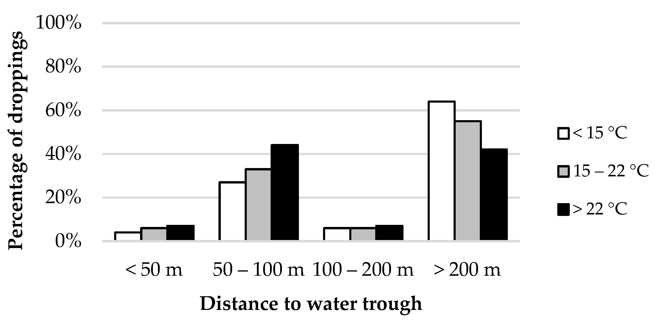
| Distance to water | <50 m | 2.22 | 3.55 | 5.92 | 0.20 ± 0.18 c | 0.20 ± 0.29 b | |
| 50–100 m | 6.45 | 16.21 | 36.70 | 0.46 ± 0.11 d | 0.64 ± 0.12 c | *** | |
| 100–200 m | 15.62 | 8.81 | 6.43 | −0.32 ± 0.07 a | −0.50 ± 0.20 a | *** | |
| >200 m | 75.71 | 71.43 | 50.95 | −0.10 ± 0.11 b | −0.36 ± 0.18 a | *** |
| Spatial Domain | Temporal Domain | GPS Variable | CONS | Coefficients * | R2 | MAEc ** | MAEv ** | |||||
|---|---|---|---|---|---|---|---|---|---|---|---|---|
| GPS | CC | DW | IN | NDVI | SL | |||||||
| 1 plot | 1 week | - | 3.382 | −0.003 | −0.097 | 0.097 | 1.324 | 1.912 | ||||
| 1 plot | 1 week | fix | 2.172 | 0.479 *** | −0.002 | −0.059 | 0.321 | 1.116 | 1.646 | |||
| 1 plot | 1 week | segment | 1.872 | 0.186 *** | −0.002 | −0.049 | 0.356 | 1.068 | 1.625 | |||
| 1 plot | 1 week | time | 1.896 | 0.935 | −0.002 | −0.053 | 0.320 | 1.092 | 1.625 | |||
| 1 plot | 6 weeks | - | 21.895 | −0.020 | −0.633 | 0.156 | 1.002 | 1.503 | ||||
| 1 plot | 6 weeks | fix | 11.282 | 0.512 | −0.009 | −0.322 | 0.508 | 0.709 | 1.116 | |||
| 1 plot | 6 weeks | segment | −0.576 | 0.173 | 0.539 | 0.687 | 1.113 | |||||
| 1 plot | 6 weeks | time | 4.879 | 1.199 | −6.785 | 0.512 | 0.862 | 1.202 | ||||
| 4 plots | 1 week | - | 18.670 | −0.013 | −0.012 | −0.586 | 0.291 | 0.864 | 1.400 | |||
| 4 plots | 1 week | fix | 5.846 | 0.697 *** | −12.760 | −0.003 | 20.025 | 0.529 | 0.679 | 1.146 | ||
| 4 plots | 1 week | segment | 4.930 | 0.250 *** | −10.092 | −0.003 | 14.484 | 0.576 | 0.636 | 1.085 | ||
| 4 plots | 1 week | time | 3.595 | 1.363 | −10.286 | 16.476 | 0.526 | 0.665 | 1.104 | |||
| 4 plots | 6 weeks | - | 99.713 | −0.087 | −3.336 | 0.380 | 0.737 | 1.303 | ||||
| 4 plots | 6 weeks | fix | 20.231 | 0.757 | −56.944 | 0.743 | 0.440 | 0.879 | ||||
| 4 plots | 6 weeks | segment | 19.528 | 0.299 *** | −46.765 | 0.828 | 0.363 | 0.802 | ||||
| 4 plots | 6 weeks | time | 17.450 | 1.590 | −48.280 | 0.773 | 0.399 | 0.850 | ||||
| Spatial Domain | Temporal Domain | GPS Variable | CONS | Coefficients * | R2 | MAEc ** | MAEv ** | |||||||
|---|---|---|---|---|---|---|---|---|---|---|---|---|---|---|
| GPS | CC | DW | IN | NDVI | SL | TA | TM | |||||||
| 1 plot | 1 week | - | 2.016 | 0.014 | −0.003 | −0.103 | 0.064 | 0.167 | 1.207 | 2.128 | ||||
| 1 plot | 1 week | point | 1.742 | 0.366 | −0.005 | −0.002 | −0.002 | −0.061 | 0.052 | 0.451 | 1.058 | 1.984 | ||
| 1 plot | 1 week | segment | 1.033 | 0.122 | −0.001 | −0.003 | −0.055 | 0.045 | 0.470 | 2.237 | 3.003 | |||
| 1 plot | 1 week | time | 1.769 | 0.797 | −0.007 | −0.001 | −0.003 | −0.058 | 0.049 | 0.471 | 1.100 | 2.063 | ||
| 1 plot | 6 weeks | - | −9.061 | 9.141 | −0.021 | −0.651 | 0.865 | 0.293 | 0.934 | 1.790 | ||||
| 1 plot | 6 weeks | point | −8.697 | 0.408 | −4.843 | −0.009 | −0.017 | −0.356 | 0.747 | 0.746 | 0.587 | 1.558 | ||
| 1 plot | 6 weeks | segment | 2.686 | 0.142 | −0.024 | −18.290 | −0.302 | 0.394 | 0.779 | 0.527 | 1.635 | |||
| 1 plot | 6 weeks | time | −7.385 | 0.839 | −4.902 | −0.009 | −0.018 | −0.354 | 0.710 | 0.760 | 0.554 | 1.538 | ||
| 4 plots | 1 week | - | 29.546 | −21.261 | −0.016 | −0.058 | −30.183 | −0.715 | 0.333 | 0.360 | 1.241 | 1.603 | ||
| 4 plots | 1 week | point | 11.772 | 0.913 *** | −29.115 | −0.036 | −19.093 | 0.217 | 0.590 | 0.900 | 1.234 | |||
| 4 plots | 1 week | segment | 9.053 | 0.332 *** | −22.751 | −0.029 | −18.016 | 0.197 | 0.641 | 0.844 | 1.124 | |||
| 4 plots | 1 week | time | 11.994 | 1.850 *** | −28.989 | −0.036 | −17.675 | 0.197 | 0.600 | 0.894 | 1.223 | |||
| 4 plots | 6 weeks | - | 129.717 | −0.167 | −3.777 | 0.323 | 1.170 | 0.886 | ||||||
| 4 plots | 6 weeks | point | 31.117 | 1.073 *** | −93.624 | 0.657 | 0.722 | 0.572 | ||||||
| 4 plots | 6 weeks | segment | 12.547 | 0.393 *** | 0.707 | 0.597 | 0.557 | |||||||
| 4 plots | 6 weeks | time | 31.002 | 2.140 *** | −92.531 | 0.667 | 0.712 | 0.522 | ||||||
Publisher’s Note: MDPI stays neutral with regard to jurisdictional claims in published maps and institutional affiliations. |
© 2022 by the authors. Licensee MDPI, Basel, Switzerland. This article is an open access article distributed under the terms and conditions of the Creative Commons Attribution (CC BY) license (https://creativecommons.org/licenses/by/4.0/).
Share and Cite
Hassan-Vásquez, J.A.; Maroto-Molina, F.; Guerrero-Ginel, J.E. GPS Tracking to Monitor the Spatiotemporal Dynamics of Cattle Behavior and Their Relationship with Feces Distribution. Animals 2022, 12, 2383. https://doi.org/10.3390/ani12182383
Hassan-Vásquez JA, Maroto-Molina F, Guerrero-Ginel JE. GPS Tracking to Monitor the Spatiotemporal Dynamics of Cattle Behavior and Their Relationship with Feces Distribution. Animals. 2022; 12(18):2383. https://doi.org/10.3390/ani12182383
Chicago/Turabian StyleHassan-Vásquez, Jessica A., Francisco Maroto-Molina, and José E. Guerrero-Ginel. 2022. "GPS Tracking to Monitor the Spatiotemporal Dynamics of Cattle Behavior and Their Relationship with Feces Distribution" Animals 12, no. 18: 2383. https://doi.org/10.3390/ani12182383
APA StyleHassan-Vásquez, J. A., Maroto-Molina, F., & Guerrero-Ginel, J. E. (2022). GPS Tracking to Monitor the Spatiotemporal Dynamics of Cattle Behavior and Their Relationship with Feces Distribution. Animals, 12(18), 2383. https://doi.org/10.3390/ani12182383