A Robust Method Based on Dual Encoders to Eliminate Velocity Ripple for Modular Drive Joints

Abstract

Velocity ripple is one of the common problems of modular drive joints, which easily induces vibration and noise and affects motion accuracy. In order to improve the motion control accuracy, a robust method based on dual encoders to eliminate velocity ripple is proposed in this paper. The method contains a velocity ripple elimination controller (VREC), a rigid-body velocity solver (RBVS), and a proportional–integral (PI) controller. Feeding back the VREC output to the PI controller based on the rigid-body velocity obtained from the weighted sum of dual encoders in the RBVS, an equivalent system damping term was added into the system. Therefore, the velocity ripple can be suppressed effectively with the adjustable damping term composed of control parameters. Above all, the proposed method has only one more parameter to further eliminate velocity ripple compared to the pure PI method and, meanwhile, has apparent advantages over the conventional method, such as fewer parameters and full frequency ripple elimination, as well as robustness to input disturbance and modular drive joint load inertia changes. This proposed method’s effectiveness is verified by simulations in MATLAB and experiments in the modular drive joint platform.

1. Introduction

Modular drive joints are now widely used in industrial robots and collaborative robots, integrating high efficiency and high power density permanent magnet synonym motors (PMSMs), harmonic drive, torque sensors, shafts, bearings, dual encoders, and other components [1,2,3]. The PMSM is widely employed in modular drive joints due to its advantages: fast dynamics, high efficiency and reliability, and a favorable torque to inertia ratio [4,5,6]. However, the torque ripple in the PMSM and the stiffness of the modular drive joint influenced by the flexpline of harmonic drive easily induce velocity ripple [7,8]. Furthermore, the velocity ripple will result in vibration, noise, and other similar problems, which are major factors affecting the accuracy of the motion control system [9]. In the last few years, many kinds of research have been done on the accuracy of motion control, where the velocity ripple has been found to be a major issue [10].

The factors that cause the velocity ripple of modular drive joints can mainly be divided into two categories. The first category is caused by the position measuring errors because the feedback velocity signal is usually calculated from the measured position signal [11,12]. Many algorithms were introduced to correct the position measuring error under certain conditions but with no systematic description for measuring the position measuring error on the velocity ripple in the servo system [13,14]. The other category is caused by the inevitable parasitic torque ripple in the PMSM, such as cogging and flux harmonics, leading to velocity ripples, vibrations, acoustic noise, and poor response performance in motion control systems [5,15].

Aiming to minimize torque ripple and realize velocity ripple elimination, the methods can also mainly be classified in two ways: one way is to optimize the design or improve the body structure of the PMSM [16,17,18,19], and the other way is to depend on control algorithms. The former mainly involves skewing the slot or magnet, ensuring a fractional number of slots per pole, and improving the winding distribution. These methods are proven to be effective for eliminating the velocity ripple but require complex production processes. Besides, once the designed and optimized body structure is produced, the modular drive joint cannot be modified, which results in a higher production cost [20,21]. The control algorithms of the latter way mainly contain sensorless methods and sensor-based methods. The sensorless methods control the current phase indirectly by controlling the voltage–current phase deference based on the V/f control [22,23,24]. However, if the load inertia varies depending on the joint position, such as robot posture changing, the other velocity ripple will occur easily [25].

On the contrary, the sensor-based methods are the main approaches to eliminating velocity ripple, which mainly include traditional proportion-integral-differential (PID) methods and improved PID methods, intelligent methods, and model-based methods. The traditional methods, such as PI velocity control and cascade control structure (CCS) based on PI controllers, are simple and easily achieve velocity ripple but with limited efficiency [5]. The intelligent methods include: adaptive fuzzy control methods [2,26,27] and neural network algorithms [28] with robust performance, iterative learning control (ILC) methods as a model-free control strategy to suppress velocity ripple and that is robust to noise [29,30], and a linear parameter varying $H_{\infty }$ velocity control method with robustness against disturbance characteristics [31]. These methods achieve robustness against velocity ripple and disturbances, but with a large amount of data calculation and poor real-time performance. In recent years, model-based methods have been developed, including model predictive control (MPC) methods, observer-based control methods, sliding mode control methods, and so on. These methods have advantages such as robustness, simple modeling, and the ability to handle control variable constraints to ensure the system’s satisfactory performance [7].

Among the model-based methods, the methods based on the equivalent rigid-body velocity method [32] and self-resonance cancellation (SRC) methods [33,34] are more popular. The equivalent rigid-body velocity method aims to add system damping to eliminate velocity ripple. The SRC method aims to achieve a rigid-body system by the weighted sum of sensor signals: dual encoders (motor-side encoder and link-side encoder). Base on the dual encoders of the modular drive joint, the rigid-body velocity can be obtained. The conventional method based on equivalent rigid-body velocity added an equivalent damping term after the closed loop to suppress velocity ripple. However, it only can suppress a limited frequency range ripple of velocity. To improve the conventional equivalent rigid-body velocity method, a method based on a state observer to suppress velocity ripple in the full frequency range ripple was proposed in [35]. As for the SRC methods, there are fewer control parameters but there are high requirements for system model identification accuracy, which is challenging to apply in practical engineering applications with the low accuracy of system identification.

A method combined with the ideas of the equivalent rigid-body velocity method and SRC method is proposed to add system damping with fewer control parameters in this paper. The proposed method contains a rigid-body velocity solver (RBVS), a velocity ripple elimination controller (VREC), and a proportional–integral (PI) controller. As the feedback velocity can be motor velocity or link velocity, the proposed method can be further classed as a motor-side controller and link-side controller. In the proposed method, the RBVS obtains a rigid-body velocity based on the signals of dual encoders (motor velocity measured by the motor-side encoder and link velocity measured by the link-side encoder) without any control parameters. The VREC is based on the RBVS to add an equivalent system damping term and constant term, which eliminates velocity ripple and input disturbance effectively and, meanwhile, increases the robustness to modular drive joint load inertia changes. The added equivalent damping term consists of system parameters and control parameters, which can be increased or decreased with the adjustment of control parameters. In this paper, the velocity ripple suppression effects are confirmed in a modular drive joint with variable velocity tracking in simulations and experiments with a motor-side controller and link-side controller, respectively. Furthermore, the damped input disturbance and robustness to load inertia changes are also verified by simulations and experiments with a motor-side controller and link-side controller, respectively.

This paper is organized as follows. The dynamic model and system identification of a modular drive joint are described in Section 2. The proposed method is designed and the controller parameters are analyzed in Section 3. Section 4 includes simulations and experiments of the motor-side controller and link-side controller to verify the velocity ripple elimination effects, input disturbance suppression effects, and the robust performance to load inertia changes. Finally, Section 5 concludes this paper.

2. Dynamic Modeling and System Identification

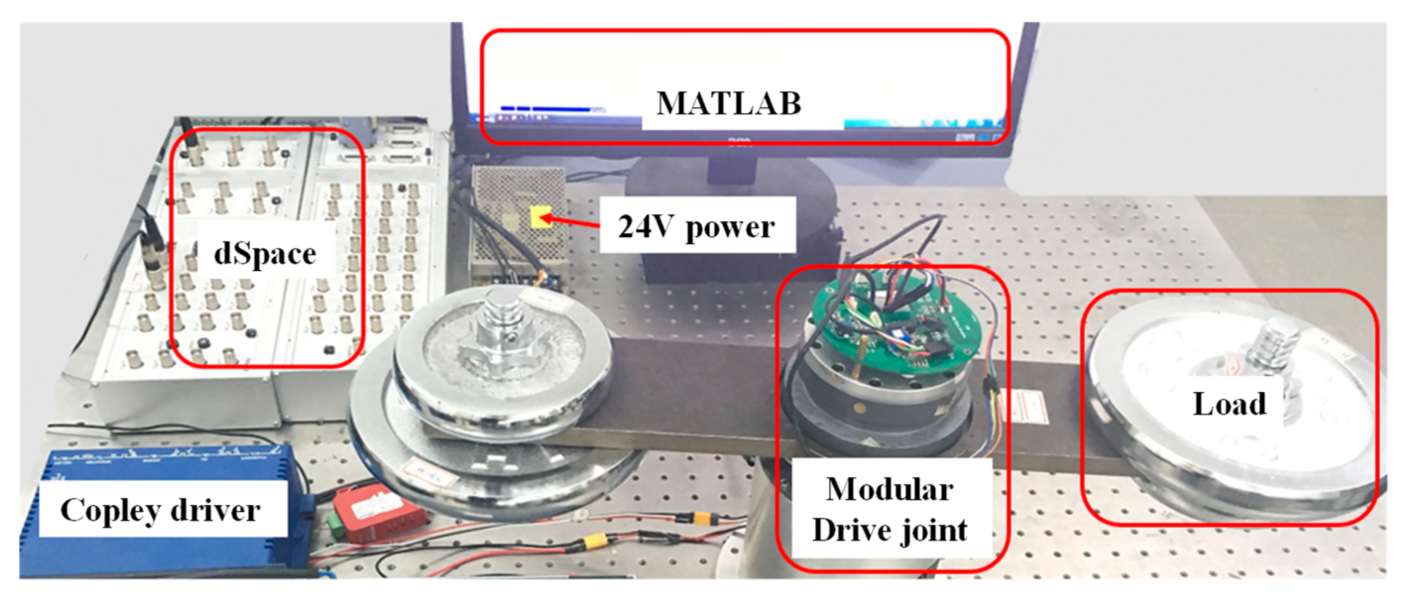
The modular drive joint is widely used in most collaborative robots as the core part, integrating electronic circuits and other mechanical components. The mechanical structure is described in [35,36]. Figure 1 shows the experimental platform based on a modular drive joint together with dSpace hardware in the loop real-time simulation platform and MATLAB real-time workspace. The actuator of the modular drive joint is the Copley driver. This experimental platform’s power is 24 V. The weights installed at both ends of the connecting rod act as the load inertia.

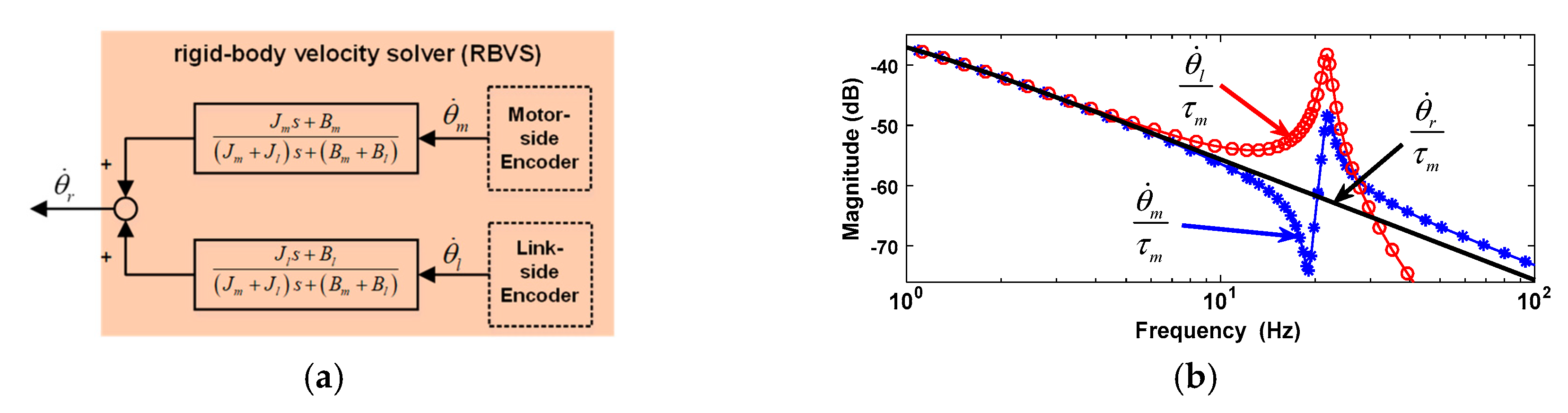
Figure 2 shows that the gear ratio of harmonic drive in the modular drive joint is equivalent to 1 [35]. Therefore, the dynamic response of this two-inertia system can be simplified as Equation (1).

$$\{\begin{array}{l}{\tau }_m-{\tau }_{dis}-{\tau }_j=J_m{\ddot{\theta }}_m+B_m{\dot{\theta }}_m\\ {\tau }_j=K\left({\theta }_m-{\theta }_l\right)+D\left({\dot{\theta }}_m-{\dot{\theta }}_l\right)\\ {\tau }_j=J_l{\ddot{\theta }}_l+B_l{\dot{\theta }}_l\end{array}$$

(1)

The physical meanings of $J_m,\hspace{0.17em}\hspace{0.17em}{B}_m,\hspace{0.17em}\hspace{0.17em}{J}_l,\hspace{0.17em}\hspace{0.17em}{B}_l,\hspace{0.17em}\hspace{0.17em}K,\hspace{0.17em}\hspace{0.17em}D,\hspace{0.17em}\hspace{0.17em}{\tau }_m,\hspace{0.17em}\hspace{0.17em}{\tau }_j,\hspace{0.17em}\hspace{0.17em}{\tau }_{dis},\hspace{0.17em}\hspace{0.17em}{\theta }_m,\hspace{0.17em}\hspace{0.17em}{\theta }_l,\hspace{0.17em}\hspace{0.17em}{\dot{\theta }}_m,\hspace{0.17em}\hspace{0.17em}{\dot{\theta }}_l,\hspace{0.17em}\hspace{0.17em}{\ddot{\theta }}_m,\hspace{0.17em}\hspace{0.17em}{\ddot{\theta }}_l$ are motor inertia, motor viscous damping, load inertia, load viscous damping, joint stiffness, joint viscous damping, input torque, joint torque, input disturbance, motor position, link position, motor velocity, link velocity, motor acceleration, and link acceleration, respectively. The transfer function from input torque ${\tau }_m$ to motor velocity ${\dot{\theta }}_m$ and link velocity ${\dot{\theta }}_l$ in the Laplace domain can be formulated as follows.

$$\{\begin{array}{l}{P}_{TM}(\mathrm{s})=\frac{{\dot{\theta }}_m}{{\tau }_m}=\left(\frac{1}{J_m+J_l}\cdot \frac{1}{s}\right)\cdot \left(\frac{s^2+{\omega }_a{}^2}{{\omega }_a{}^2}\cdot \frac{{\omega }_r{}^2}{s^2+{\omega }_r{}^2}\right)\\ P_{TL}(\mathrm{s})=\frac{{\dot{\theta }}_l}{{\tau }_m}=\left(\frac{1}{J_m+J_l}\cdot \frac{1}{s}\right)\cdot \left(\frac{{\omega }_r{}^2}{s^2+{\omega }_r{}^2}\right)\end{array}$$

(2)

where ${\omega }_a=\sqrt{K/J_l},\hspace{0.17em}{\omega }_r={\omega }_a\sqrt{1+J_l/J_m}$.

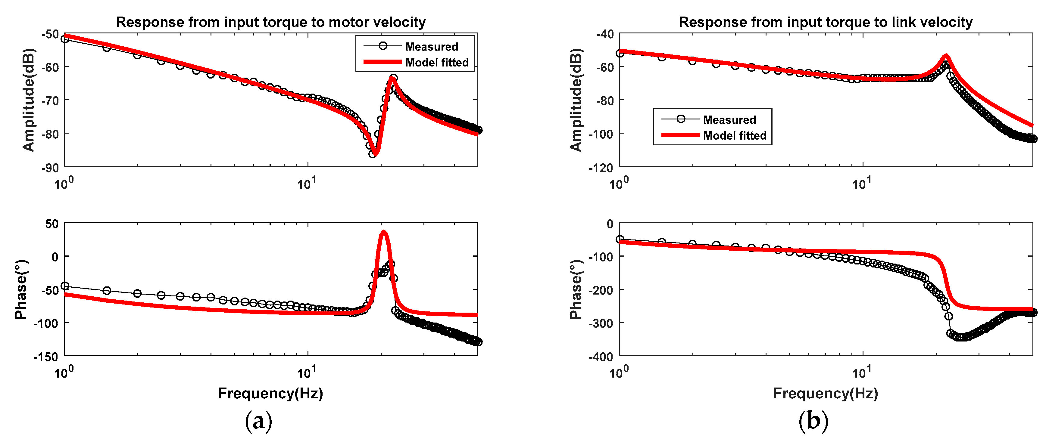
In order to verify that this two-inertia model can fit the actual modular drive joint well, a swept sine current signal is utilized to estimate the joint frequency response, with a load inertia of $J_l=2.26$ kg·m². In experiments, the sampling frequency is 1 kHz. As for the modular drive joint, the current torque constant is tested to be 0.17 N·m/A. The input saturation current is set to 10 A. The maximum velocity of the motor side is 2500 rpm. Moreover, the gear ratio of the harmonic drive is 160. After the identification experiment, the joint frequency response from input torque ${\tau }_m$ to motor velocity ${\dot{\theta }}_m$ and link velocity ${\dot{\theta }}_l$ can be obtained as shown in Figure 3a,b, respectively.

In Figure 3, the black lines are acquired by actual measurement data of the experiment. The red lines are fitted frequency response curves of the two-inertia model. The motor-side velocity response has a clear anti-resonance and resonance behavior from the identified results, whereas the link-side velocity only has a resonance behavior. In fact, the actual joint dynamic model is subjected to several nonlinear and time-varying factors, such as the nonlinear torques, frictions, and damping effects in the motor side and transmission, and the varying efficiency of harmonic drive (60–75% depending on ratio, velocity, and lubricant). In particular, the stiffness and damping of harmonic drive are related to the motion velocity. Therefore, the two-inertia model cannot fit the phase of actual system characteristics well [37]. However, the amplitude–frequency fitting accuracy can accurately fit the system’s anti-resonance and resonance characteristics, proving that the two-inertia model can reflect the joint’s dynamic characteristics well. The anti-resonance frequency ${\omega }_a$ and resonance frequency ${\omega }_r$ are located at 19 Hz and 21 Hz, respectively. Next, the identified parameters of this modular drive joint are summarized in

Table 1. Identified modular drive joint parameters.

Symbol	Name	Value
Jm	motor inertia	7.34 kg·m2
Bm	motor viscous damping	33.28 N·m·s/rad
Jl	load inertia	2.26 kg·m2
Bl	load viscous damping	5 N·m·s/rad
K	joint stiffness	34,000 N·m/rad
D	joint viscous damping	10 N·m·s/rad

.

3. Controller Design

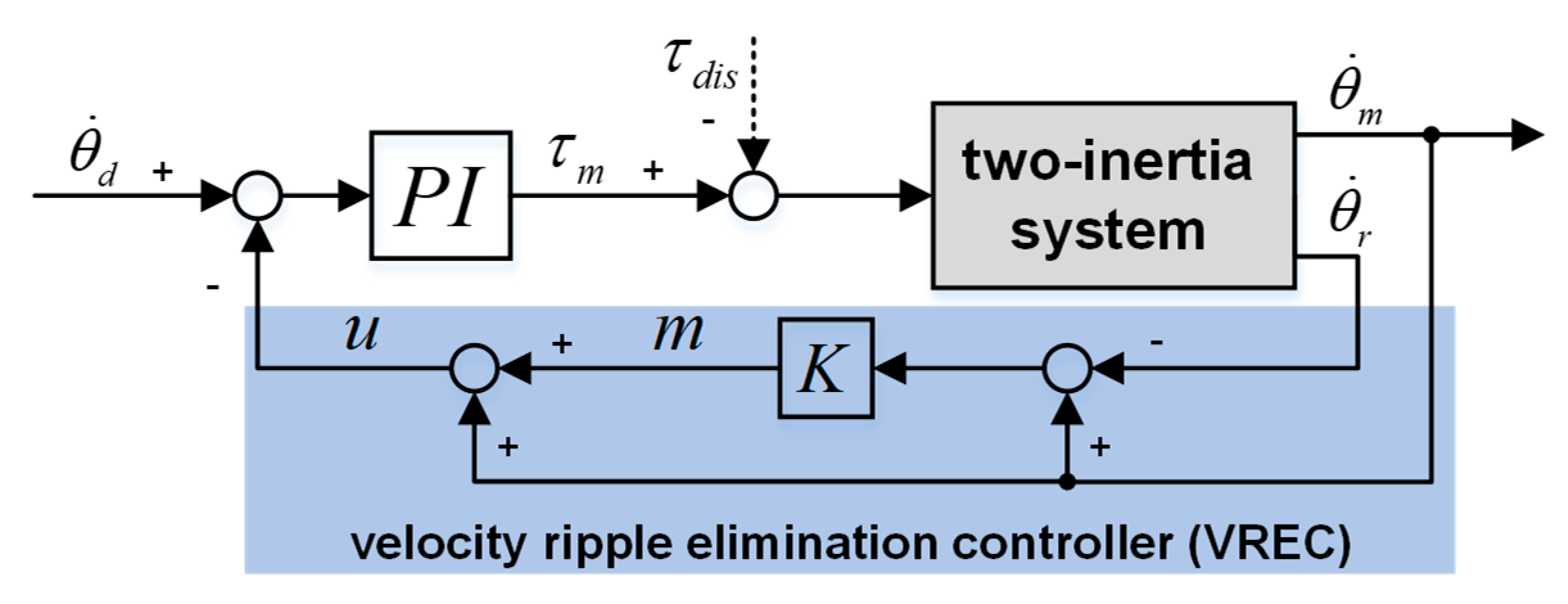
The proposed method in this paper contains an RBVS, a VREC, and a PI controller, as shown in Figure 4, and aims to eliminate velocity ripple by adding equivalent system damping. The added equivalent damping term is developed by feeding back the velocity $u$ of VREC output to the PI controller. As for the RBVS, rigid-body velocity ${\dot{\theta }}_r$ can be obtained by the weighted sum of motor velocity ${\dot{\theta }}_m$ and link velocity ${\dot{\theta }}_l$. The PI controller is a proportional and integral controller for the error between the desired velocity ${\dot{\theta }}_d$ and output velocity $u$. The VREC comprises pure ripple ($m$ or $n$) and joint velocity (motor velocity or link velocity). The pure ripple $m$ is the error between motor velocity and rigid-body velocity. As well as the pure ripple, $n$ is the error between link velocity and rigid-body velocity. Therefore, according to the joint velocity, the proposed method can be classed as the motor-side controller and link-side controller, as shown in Figure 4a,b, respectively.

In Figure 4, the model $P_M$ defines transfer function from input torque ${\tau }_m$ to motor velocity ${\dot{\theta }}_m$. Meanwhile, the model $P_{ML}$ defines transfer function from motor velocity ${\dot{\theta }}_m$ to link velocity ${\dot{\theta }}_l$, as shown in Equation (3).

$$\{\begin{array}{l}{P}_M=\frac{{\dot{\theta }}_m}{{\tau }_m}=\left(\frac{1}{J_m+J_l}\cdot \frac{1}{s}\right)\cdot \left(\frac{s^2+{\omega }_a{}^2}{s^2+{\omega }_r{}^2}\cdot \frac{{\omega }_r{}^2}{{\omega }_a{}^2}\right)\\ P_{ML}=\frac{{\dot{\theta }}_l}{{\dot{\theta }}_m}=\frac{{\omega }_a{}^2}{s^2+{\omega }_a{}^2}\end{array}$$

(3)

Besides, the PI controller and coefficients $\alpha$ and $\beta$ of the RBVS are defined as follows, which will be discussed in the next section:

$$\{\begin{array}{l}PI=K_p+\frac{K_i}{s}\\ \alpha =\frac{J_{m}s+B_m}{\left(J_m+J_l\right)s+\left(B_m+B_l\right)}\\ \beta =\frac{J_{l}s+B_l}{\left(J_m+J_l\right)s+\left(B_m+B_l\right)}\end{array}$$

(4)

3.1. Rigid-Body Velocity Solver Design

The rigid-body velocity ${\dot{\theta }}_r$ is obtained based on the weighted sum of motor velocity and link velocity in the rigid-body velocity solver. Combined with the two-inertia model that has been given in Equation (1), rigid-body velocity ${\dot{\theta }}_r$ can be derived from Equation (5). The input disturbance ${\tau }_{dis}$ is not discussed at this time and is set to zero for simplicity. Among them, motor velocity is measured by the motor-side encoder. Link velocity is measured by the link-side encoder, as shown in Figure 5a.

$$\{\begin{array}{l}{J}_m{\ddot{\theta }}_m+B_m{\dot{\theta }}_m={\tau }_m-K\left({\theta }_m-{\theta }_l\right)+D\left({\dot{\theta }}_m-{\dot{\theta }}_l\right)\\ J_l{\ddot{\theta }}_l+B_l{\dot{\theta }}_l=K\left({\theta }_m-{\theta }_l\right)+D\left({\dot{\theta }}_m-{\dot{\theta }}_l\right)\\ {\tau }_m=\left(J_{m}s+B_m\right){\dot{\theta }}_m+\left(J_{l}s+B_l\right){\dot{\theta }}_l\\ {\dot{\theta }}_r=\frac{{\tau }_m}{\left(J_m+J_l\right)s+\left(B_m+B_l\right)}=\frac{J_{m}s+B_m}{\left(J_m+J_l\right)s+\left(B_m+B_l\right)}{\dot{\theta }}_m+\frac{J_{l}s+B_l}{\left(J_m+J_l\right)s+\left(B_m+B_l\right)}{\dot{\theta }}_l\end{array}$$

(5)

The transfer function from input torque ${\tau }_m$ to rigid-body velocity ${\dot{\theta }}_r$ can be obtained by:

$$\frac{{\dot{\theta }}_r}{{\tau }_m}=\frac{1}{\left(J_m+J_l\right)s+\left(B_m+B_l\right)}=\frac{J_{m}s+B_m}{\left(J_m+J_l\right)s+\left(B_m+B_l\right)}\frac{{\dot{\theta }}_m}{{\tau }_m}+\frac{J_{l}s+B_l}{\left(J_m+J_l\right)s+\left(B_m+B_l\right)}\frac{{\dot{\theta }}_l}{{\tau }_m}$$

(6)

From Equations (2) and (6), the Bode diagram shows the transfer function from input torque ${\tau }_m$ to motor velocity ${\dot{\theta }}_m$, link velocity ${\dot{\theta }}_l$ and rigid-body velocity ${\dot{\theta }}_r$ in Figure 5b, as the blue line, red line, and thick black line, respectively. As the modular drive joint identified results listed in Table 1, the motor viscous damping is higher than link viscous damping, which leads to the magnitude of motor velocity frequency response being lower than the link velocity frequency response.

As stated by the Bode diagram from input torque ${\tau }_m$ to rigid-body velocity ${\dot{\theta }}_r$, there are no anti-resonance and resonance behaviors. Consequently, the system from input torque ${\tau }_m$ to rigid-body velocity ${\dot{\theta }}_r$ is an ideal rigid-body system without any velocity ripple. The velocity obtained from the weighted sum of motor velocity and link velocity is an ideal rigid-body velocity.

3.2. Velocity Ripple Elimination Controller Design

3.2.1. Motor-Side Controller Design

Based on the rigid-body velocity discussed in Section 3.1, the motor-side controller can be simplified as a PI controller and a VREC. The VREC feeds back the velocity $u$ to the desired velocity ${\dot{\theta }}_d$ input to the PI controller. The pure ripple $m$ is obtained from the error between motor velocity and rigid-body velocity after the proportional gain $K$ tuning, as shown in Figure 6.

In Figure 6, the signal $m$ is pure the ripple of motor velocity after being controlled by $K$. The symbol $u$ is the sum of motor velocity and pure ripple $m$. The input disturbance ${\tau }_{dis}$ is not discussed for simplicity. Then the open-loop transfer function $P_{open}{}^m(\mathrm{s})$ from the desired velocity ${\dot{\theta }}_d$ to motor velocity ${\dot{\theta }}_m$ can be given in Equation (7).

$$P_{open}{}^m(\mathrm{s})=\frac{{\dot{\theta }}_m}{{\dot{\theta }}_d}=\frac{PI{\omega }_r{}^2}{\left(J_m+J_l\right)s\cdot \left(s^2+{\omega }_r{}^2\right)}\frac{\left(s^2+{\omega }_a{}^2\right)}{{\omega }_a{}^2}$$

(7)

The closed-loop transfer function $P_{close}{}^m(\mathrm{s})$ from the desired velocity ${\dot{\theta }}_d$ to motor velocity ${\dot{\theta }}_m$ can be derived from the following equations.

$$\{\begin{array}{l}\left({\dot{\theta }}_d-u\right)P_{open}{}^m={\dot{\theta }}_m\\ u={\dot{\theta }}_m+m\\ m=K\left({\dot{\theta }}_m-{\dot{\theta }}_r\right)\\ {\dot{\theta }}_r=\alpha {\dot{\theta }}_m+\beta {\dot{\theta }}_l\\ {\dot{\theta }}_l={\dot{\theta }}_m{P}_{ML}\end{array}$$

(8)

$$\begin{array}{l}{P}_{close}{}^m(\mathrm{s})=\frac{{\dot{\theta }}_m}{{\dot{\theta }}_d}=\frac{P_{open}{}^m}{1+P_{open}{}^m\left[1+K\left(1-\alpha -\beta P_{ML}\right)\right]}\\ \hspace{1em}\hspace{0.17em}\hspace{0.17em}\hspace{0.17em}\hspace{1em}\hspace{1em}\hspace{1em}\hspace{0.17em}\hspace{0.17em}\hspace{0.17em}=\frac{\frac{PI\left(s^2+{\omega }_a{}^2\right){\omega }_r{}^2}{\left(J_m+J_l\right)\left(s^2+{\omega }_r{}^2\right){\omega }_a{}^{2}s}}{1+\frac{PI\left(s^2+{\omega }_a{}^2\right){\omega }_r{}^2}{\left(J_m+J_l\right)\left(s^2+{\omega }_r{}^2\right){\omega }_a{}^{2}s}\left[1+K\left(1-\frac{\left(J_{m}s+B_m\right)\left(s^2+{\omega }_a{}^2\right)-\left(J_{l}s+B_l\right){\omega }_a{}^2}{\left[\left(J_m+J_l\right)s+\left(B_m+B_l\right)\right]\left(s^2+{\omega }_a{}^2\right)}\right)\right]}\end{array}$$

(9)

In order to analyze the closed-loop transfer function performance of the motor-side controller, the viscous damping terms $B_m,\hspace{0.17em}{B}_l,\hspace{0.17em}D$ are set to zero for simplicity. Then the closed-loop transfer function $P_{close}{}^m(\mathrm{s})$ can be simplified, as in Equation (10).

$$\{\begin{array}{l}{P}_{close}{}^m(\mathrm{s})=\frac{{\dot{\theta }}_m}{{\dot{\theta }}_d}=\frac{PI{\omega }_r{}^2}{\left(J_m+J_l\right)s\cdot \left(s^2+2{\xi }_m{\omega }_{r}s+{\omega }_r{}^2\right)+PI{\omega }_r{}^2}\frac{\left(s^2+{\omega }_a{}^2\right)}{{\omega }_a{}^2}\\ {\xi }_m=\frac{PI}{2}\left[\frac{K}{{\omega }_r}\left(\frac{{\omega }_r{}^2}{{\omega }_a{}^2}-1\right)+\frac{{\omega }_r}{\left(J_m+J_l\right){\omega }_a{}^2}\right]\end{array}$$

(10)

Based on the modular drive joint identified results, the resonance frequency ${\omega }_r$ is always larger than the anti-resonance frequency ${\omega }_a$, which leads to ${\omega }_r{}^2/{\omega }_a{}^2$ being more than 1 and ${\xi }_m$ being positive permanently. Compared with the open-loop transfer function given in Equation (7), the closed-loop transfer function has an added equivalent damping term $2{\xi }_m{\omega }_{r}s$ and an equivalent natural resonance term $PI{\omega }_r{}^2$, which increase system damping and system response performance, respectively. With the control parameter $K$ being positive, the velocity ripple can be eliminated by the increased equivalent damping.

3.2.2. Link-Side Controller Design

Similarly, when the pure ripple $n$ is obtained from the error between link velocity and rigid-body velocity, there could be a link-side controller to eliminate the velocity ripple by feeding back this error and link velocity to the PI controller, as shown in Figure 7.

In Figure 7, the signal $n$ is the pure ripple of link velocity after being controlled by $K$. The symbol $u$ is the sum of link velocity and pure ripple $n$. The input disturbance ${\tau }_{dis}$ is not discussed for simplicity. The open-loop transfer function $P_{open}{}^m(\mathrm{s})$ from the desired velocity ${\dot{\theta }}_d$ to link velocity ${\dot{\theta }}_l$ can be given by Equation (11).

$$P_{open}{}^l(\mathrm{s})=\frac{{\dot{\theta }}_l}{{\dot{\theta }}_d}=\frac{PI{\omega }_r{}^2}{\left(J_m+J_l\right)s\cdot \left(s^2+{\omega }_r{}^2\right)}$$

(11)

The closed-loop transfer function $P_{close}{}^l(\mathrm{s})$ from the desired velocity ${\dot{\theta }}_d$ to link velocity ${\dot{\theta }}_l$ can be derived from the following.

$$\{\begin{array}{l}\left({\dot{\theta }}_d-u\right)P_{open}{}^m={\dot{\theta }}_l\\ u={\dot{\theta }}_l+n\\ n=K\left({\dot{\theta }}_l-{\dot{\theta }}_r\right)\\ {\dot{\theta }}_r=\alpha {\dot{\theta }}_m+\beta {\dot{\theta }}_l\\ {\dot{\theta }}_m=\frac{{\dot{\theta }}_l}{P_{ML}}\end{array}$$

(12)

$$\begin{array}{l}{P}_{close}{}^l(\mathrm{s})=\frac{{\dot{\theta }}_l}{{\dot{\theta }}_d}=\frac{P_{open}{}^l}{1+P_{open}{}^l\left[1+K\left(1-\frac{\alpha }{P_{ML}}-\beta \right)\right]}\\ \hspace{1em}\hspace{1em}\hspace{0.17em}\hspace{1em}\hspace{1em}\hspace{1em}\hspace{0.17em}=\frac{\frac{PI{\omega }_r{}^2}{\left(J_m+J_l\right)\left(s^2+{\omega }_r{}^2\right)s}}{1+\frac{PI{\omega }_r{}^2}{\left(J_m+J_l\right)\left(s^2+{\omega }_r{}^2\right)s}\left[1+K\left(1-\frac{\left(J_{m}s+B_m\right)\left(s^2+{\omega }_a{}^2\right)-\left(J_{l}s+B_l\right){\omega }_a{}^2}{\left[\left(J_m+J_l\right)s+\left(B_m+B_l\right)\right]{\omega }_a{}^2}\right)\right]}\end{array}$$

(13)

Correspondingly, the viscous damping terms $B_m,\hspace{0.17em}{B}_l,\hspace{0.17em}D$ are ignored for simplicity to analyze the closed-loop transfer function performance of the link-side controller. Therefore, the closed-loop transfer function $P_{close}{}^l(\mathrm{s})$ can be simplified, as shown in Equation (14).

$$\{\begin{array}{l}{P}_{close}{}^l(\mathrm{s})=\frac{{\dot{\theta }}_l}{{\dot{\theta }}_d}=\frac{PI{\omega }_r{}^2}{\left(J_m+J_l\right)s\cdot \left(s^2+2{\xi }_l{\omega }_{r}s+{\omega }_r{}^2\right)+PI{\omega }_r{}^2}\\ {\xi }_l=\frac{-K\cdot PI}{2{\omega }_r}\end{array}$$

(14)

Compared to the open-loop transfer function given in Equation (11), the closed-loop transfer function adds an equivalent damping term $2{\xi }_l{\omega }_{r}s$ and an equivalent natural resonance term $PI{\omega }_r{}^2$. When the $K$ is negative, the added equivalent damping term becomes positive, and then the system damping can be increased. With the control parameter $K$ and $PI$ tuning, the velocity ripple can be eliminated by the increased equivalent damping.

3.3. Controller Parameter Analysis

In the proposed method, as discussed above, the motor-side controller and link-side controller have only one more control parameter $K$ than a PI method. The PI method can also include two kinds of feedback (motor velocity feedback and link velocity feedback), as shown in Figure 8a,b, respectively.

Firstly, the PI parameters need to be designed before the proposed method application. Based on the integral of squared error (ISE) criterion [38], the proportional and integral gain of the motor velocity feedback PI controller are designed as $K_p=480$ and $K_i=2400$. The proportional and integral gain of the link velocity feedback PI controller are designed as $K_p=168$ and $K_i=1200$.

3.3.1. Parameters of Motor-Side Controller

For a modular drive joint, the elimination of velocity ripple is mainly to suppress velocity ripple occurring on the link side. This is based on the closed-loop transfer function from the desired velocity to motor velocity with the motor-side controller, as expressed in Equation (10) and Figure 6. Naturally, the transfer function from the desired velocity to link velocity can be given by Equation (15).

$$\{\begin{array}{l}{P}_{close}{}^m(\mathrm{s})=\frac{{\dot{\theta }}_l}{{\dot{\theta }}_d}=\frac{{\dot{\theta }}_m}{{\dot{\theta }}_d}\cdot P_{ML}=\frac{PI{\omega }_r{}^2}{\left(J_m+J_l\right)s\cdot \left(s^2+2{\xi }_m{\omega }_{r}s+{\omega }_r{}^2\right)+PI{\omega }_r{}^2}\\ {\xi }_m=\frac{PI}{2}\left[\frac{K}{{\omega }_r}\left(\frac{{\omega }_r{}^2}{{\omega }_a{}^2}-1\right)+\frac{{\omega }_r}{\left(J_m+J_l\right){\omega }_a{}^2}\right]\end{array}$$

(15)

The closed-loop transfer function from the desired velocity to link velocity has an added equivalent damping term $2{\xi }_m{\omega }_{r}s$ and an equivalent natural resonance term $PI{\omega }_r{}^2$ compared to the open-loop transfer function. The parameter $K$ can be expressed by Equation (16).

$$K=\left(\frac{2{\omega }_r}{PI}{\xi }_m-\frac{{\omega }_r{}^2}{\left(J_m+J_l\right){\omega }_a{}^2}\right)/\left(\frac{{\omega }_r{}^2}{{\omega }_a{}^2}-1\right)$$

(16)

When the damping ratio ${\xi }_m$ of the closed-loop transfer function is under damping, critical damping, and over damping, such as ${\xi }_m=0.2$, ${\xi }_m=1$, ${\xi }_m=2$, as well as the special damping ratio ${\xi }_m=0.707$, the parameter $K$ can be obtained from Equation (16) based on the identified parameters listed in Table 1 and the above parameters $K_p$ and $K_i$, as shown in

Table 2. The parameter $K$ derived from different damping ratios ${\xi }_m$.

	Under Damping	Under Damping	Critical Damping	Over Damping
${\xi }_m$	0.2	0.707	1	2
$K$	0.08	0.87	1.41	3.28

.

The closed-loop Bode diagrams of motor-side controller from the desired velocity to motor velocity with different parameters $K$ are shown in Figure 9.

As the parameter $K$ increases (the damping ratio increases), the system damping gradually increases, which leads to the velocity ripple being damped, however, this decreases the closed-loop control bandwidth. The parameter $K$ as well as the proportional and integral gain $K_p$ and $K_i$ are designed to be those in

Table 3. Parameters of motor-side controller.

Symbol	Name	Value
$K_p$	proportional gain	480
$K_i$	integral gain	2400
$K$	gain of VREC	1.3

. Under the current parameters, the amplitude margin and phase margin of the closed-loop frequency response are sufficient. The amplitude margin and phase margin are 22.9 dB and 58.7 deg, respectively, which proves the system is stable after closed-loop control.

3.3.2. Parameters of Link-Side Controller

The link-side controller, shown in Figure 7, shows that the closed-loop transfer function from the desired velocity to link velocity is expressed in Equation (14). Based on the foregone proportional and integral gain of $K_p=168$ and $K_i=1200$, the parameter $K$ of the link-side controller can be obtained by Equation (17).

$$K=-\frac{2{\omega }_r}{PI}{\xi }_l$$

(17)

Similarly, when the damping ratio ${\xi }_l$ of the closed-loop transfer function represents under damping, critical damping, and over damping, such as ${\xi }_l=0.2$, ${\xi }_l=1$, ${\xi }_l=2$, as well as the special damping ratio ${\xi }_l=0.707$, the different parameters $K$ can be summarized in

Table 4. The parameter $K$ derived from different damping ratios ${\xi }_l$.

	Under Damping	Under Damping	Critical Damping	Over Damping
${\xi }_l$	0.2	0.707	1	2
$K$	−0.22	−0.98	−1.52	−3.21

, based on the identified parameters listed in Table 1 and the above parameters $K_p$ and $K_i$.

The closed-loop Bode diagram of the link-side controller from the desired velocity to link velocity with different parameters $K$ are shown in Figure 10.

In a similar way, with parameter $K$ increasing (damping ratio increasing), the system damping gradually increases, which lets the velocity ripple eliminate but decreases the closed-loop control bandwidth. Since there is no anti-resonance point in the transfer function from the desired velocity to link velocity, the phase will drop quickly, and the system is easy to diverge [39]. Therefore, the control parameters of the link-side controller should be very conservative. The parameter $K$ as well as the proportional–integral gain $K_p$ and $K_i$ are set in

Table 5. Parameters of link-side controller.

Symbol	Name	Value
$K_p$	proportional gain	168
$K_i$	integral gain	1200
$K$	gain of VREC	−0.9

.

4. Simulations and Experiments

Simulations and experiments are conducted to verify the effectiveness of this proposed method (named Prop method in this paper), using the modular drive joint’s identified parameters, as listed in Table 1. The control parameters of the motor-side controller and link-side controller are scheduled in Table 3 and Table 5. The experimental platform is described in Section 2. The sampling frequency of the controller and the experimental platform is 1 kHz. In simulations and experiments, a variable velocity tracking from high velocity to low velocity is used for verifying the effectiveness of velocity ripple elimination at different velocities. Next, the system stability is confirmed by an input disturbance suppression. Finally, with the load inertia changing in the range of 30% in the premise of unchangeable identified model parameters and control parameters, the robust performance is verified. This Prop method is compared with the traditional pure PI method, the conventional method (named Conv method in this paper) present in [32] and the conventional method improved in [35] based on a state observer (named Csob method in this paper), to prove its advantages.

4.1. Motor-Side Controller Simulations and Experiments

In the motor-side controller’s simulations and experiments, the modular drive joint is controlled by the PI method, Conv method, Csob method, and the Prop method. In order to fairly compare the effects of these methods, it is necessary to ensure the same proportional and integral gain of these methods. Above all, the PI method has two parameters. The Conv method has six parameters. The Csob method has four parameters. Meanwhile, the Prop method only has three parameters. The control parameters of these four methods are summarized in

Table 6. Control parameters of the four methods with motor-side controller.

Methods	$\mathbf{Proportional} \mathbf{Gain} {\mathit{K}}_{\mathit{p}}$	$\mathbf{Integral} \mathbf{Gain} {\mathit{K}}_{\mathit{i}}$	$\mathbf{High}-\mathbf{Pass} \mathbf{Filter} {\mathit{f}}_{\mathit{h}}$	$\mathbf{Low}-\mathbf{Pass} \mathbf{Filter} {\mathit{f}}_{\mathit{l}}$	$\mathbf{Inner}-\mathbf{Loop} \mathbf{Gain} {\mathit{K}}_{\mathit{m}}$	$\mathbf{Outer}-\mathbf{Loop} \mathbf{Gain} \mathit{K}$
PI method	480	2400	-	-	-	-
Conv method			${\omega }_r$	${\omega }_r$	300	1.3
Csob method			-	-	600	1.3
Prop method			-	-	-	1.3

.

4.1.1. Velocity Ripple Elimination

A motor-side desired step velocity is triggered at 0.1 s to get 1000 rpm (0.66 rad/s of link-side velocity) and keeps constant motion at this velocity, then is reduced to 500 rpm (0.33 rad/s of link-side velocity) at 1.5 s. The link velocity tracking with these four different methods in simulations and experiments is shown in Figure 11a,b, respectively. The black dotted line is link velocity tracking with the PI method. The blue dot-and-dash line is the Conv method. The green dot-and-dash line is the Csob method. The red solid thick line is the Prop method.

As the simulation results show in Figure 11a, when the velocity ripple at 0.66 rad/s is eliminated within 10%, the decay time of the Prop method is around 61% less than that of the PI method and Conv method. When the velocity ripple at 0.33 rad/s is eliminated within 10%, the decay time of the Prop method is 56% less than that of the PI method and Conv method. However, the Csob method does not work with motor velocity feedback control.

As for the experiment results shown in Figure 11b, when the velocity ripple at 0.66 rad/s is eliminated within 10%, the decay time of the Prop method is 49% less than that of the PI method and Conv method (Prop method: 0.221 s; PI method and Conv method: 0.431 s). When the velocity ripple at 0.33 rad/s is eliminated within 10%, the decay time of the Prop method is 55% less than that of the PI method and Conv method. However, the Csob method does not work with motor velocity feedback control.

In actual applications, the modular drive joint is a complex nonlinear system influenced by some nonlinear and time-varying factors, such as the nonlinear torques, frictions, damping effects, and the varying efficiency of harmonic drive. Above all, the transmission error of harmonic drive will induce velocity ripple during low-speed uniform motion, which is twice the frequency of the motion velocity [40]. In simulations, the transmission error model of harmonic drive is not modeled in the objective two-inertia model of modular drive joints, so there is no velocity ripple during low-speed uniform motion at 0.33 rad/s, shown in Figure 11a. Actually, during the uniform motion at 0.33 rad/s from 2 s to 3 s, the Prop method can effectively suppress velocity ripple in experiments. Meanwhile, with the added equivalent system damping increasing, the velocity response is slowed down, as shown in the partial enlarged drawing of Figure 11b. The Conv method has a phase adjuster, which means the Conv method can only damp a limited range of velocity ripple frequencies around the system resonance frequency. When the twice frequency of motion velocity is much lower than the system resonance frequency, the Conv method cannot eliminate the twice-frequency ripple frequency. The Csob method has a state observer to obtain the rigid-body velocity indirectly. When the observed motor velocity approaches the actual motor velocity, the rigid-body velocity can be obtained. Above all, there is a motor-side nominal model in the state observer, which means the Csob method’s bandwidth with motor velocity feedback control is limited by the anti-resonance. Under the premise of the same proportional and integral gain for a fair comparison, the Csob method’s bandwidth is much lower than the other methods. The added damping term is too small to eliminate velocity ripple with the Conv method and Csob method because the system resonance frequency is too close to the anti-resonance frequency.

4.1.2. Input Disturbance Suppression

In practical applications, the modular drive joint is influenced by some input disturbance, which reduces the control accuracy and system stability. Therefore, a 6 A shock input current is triggered at 0.1 s to act as the input disturbance, while the desired velocity is held at 0 rad/s. With the same input disturbance trigger, the suppressive effects of input disturbance with the PI method, the Conv method, the Csob method, and the Prop method in simulations and experiments are shown in Figure 12a,b, respectively. In these figures, the black dotted line is the PI method. The blue dot-and-dash line is the Conv method. The green dot-and-dash line is the Csob method. The red solid thick line is the Prop method.

As discussed above, the added equivalent damping term is too small to effectively damp input disturbance with motor velocity feedback of the Conv method and Csob method. When the velocity ripple is suppressed within 10% of the maximum velocity ripple value, the decay time of the Prop method is 45% less than the other three methods (PI method, Conv method, Csob method) in simulations and 68% less in experiments (Prop method: 0.114 s; PI method: 0.357 s).

In actual experiments, the modular drive joint is influenced by the nonlinear stiffness of harmonic drive. Especially when the modular drive joint is started and/or stopped, the nonlinear stiffness seriously affects the response performance and steady-state performance of the link-side velocity, which does not occur in simulations. Therefore, the system stabilization time after the input disturbance needs longer in experiments. Compared to simulations, the magnitude of link velocity response induced by input disturbance is much lower than that of simulations because of the actual time-varying frictions and viscous damping effects.

4.1.3. Robust Performance to Load Inertia Changes

When the collaborative robot changes poses, the modular drive joint will receive different load inertias. In simulations, with the unchangeable identified model parameters listed in Table 1 and control parameters listed in Table 3, different load inertias were taken to verify the robust performance, 15% increased ($J_l=2.60$ kg·m²) and 15% decreased ($J_l=1.92$ kg·m²), on the basis of load inertia $J_l=2.26$ kg·m². In experiments, the load inertia is changed by loading or unloading the loads (weights) at the end of the connecting rod, as shown in Figure 1.

In Figure 13, the solid red line is link velocity ripple with load inertia $J_l=2.26$ kg·m². The black dotted line is link velocity ripple with 15% increased load inertia $J_l=2.60$ kg·m². The blue dot-and-dash line is link velocity ripple with 15% decreased load inertia $J_l=1.92$ kg·m². Changing load inertia in the range of 30%, the Prop method can hold its stability and have a similar elimination effect on velocity ripple. Figure 13b shows velocity ripple during low-speed uniform motion at 0.33 rad/s, which is caused by the transmission error of harmonic drive. The transmission error model is not considered in the two-inertia model (modular drive joint model) in simulations. Therefore, there is no velocity ripple during low-speed uniform motion in simulations.

In conclusion, the simulation and experiment decay time reduced percentage effects of the Conv method, Csob method, and Prop method compared to the PI method with the motor-side controller, summarized in

Table 7. Suppression percentage of Conv, Csob, and Prop methods compared to PI method with motor-side controller.

Methods	Simulations			Experiments
	Ripple at 0.66 rad/s	Ripple at 0.33 rad/s	Input Disturbance	Ripple at 0.66 rad/s	Ripple at 0.33 rad/s	Input Disturbance
Conv	0%	0%	3%	0%	0%	5%
Csob	0%	0%	0%	0%	0%	16%
Prop	61%	56%	45%	49%	55%	68%

.

4.2. Link-Side Controller Simulations and Experiments

As for the simulations and experiments of the link-side controller, the modular drive joint is also controlled by the PI method, Conv method, Csob method, and the Prop method, which have two parameters, six parameters, four parameters, and three parameters, respectively. To fairly compare the effects of these four different methods, the same proportional and integral gain of these methods needs to be guaranteed. The control parameters of these four different methods are summarized in

Table 8. Control parameters of these four methods with link-side controller.

Methods	$\mathbf{Proportional} \mathbf{Gain} {\mathit{K}}_{\mathit{p}}$	$\mathbf{Integral} \mathbf{Gain} {\mathit{K}}_{\mathit{i}}$	$\mathbf{High}-\mathbf{Pass} \mathbf{Filter} {\mathit{f}}_{\mathit{h}}$	$\mathbf{Low}-\mathbf{Pass} \mathbf{Filter} {\mathit{f}}_{\mathit{l}}$	$\mathbf{Inner}-\mathbf{Loop} \mathbf{Gain} {\mathit{K}}_{\mathit{m}}$	$\mathbf{Outer}-\mathbf{Loop} \mathbf{Gain} \mathit{K}$
PI method	168	1200	-	-	-	-
Conv method			${\omega }_r$	${\omega }_r$	300	−0.9
Csob method			-	-	600	−0.9
Prop method			-	-	-	−0.9

.

4.2.1. Velocity Ripple Elimination

Similarly, a motor-side desired step velocity is triggered at 0.1 s to get 1000 rpm (0.66 rad/s of link-side velocity) and keeps uniform motion at this velocity, then is reduced to 500 rpm (0.33 rad/s of link-side velocity) at 1.5 s. The link velocity tracking with these four different methods in simulations and experiments is shown in Figure 14a,b, respectively. The black dotted line is link velocity tracking with the PI method. The blue dot-and-dash line is the Conv method. The green dot-and-dash line is the Csob method. The red solid thick line is the Prop method.

With the link-side controller, the Conv method and Csob method have obvious effects compared to the motor-side controller. The added equivalent damping term is only related to the system resonance frequency but not related to the system anti-resonance frequency. As the simulation results show in Figure 14a, when the velocity ripple at 0.66 rad/s is eliminated within 10%, the decay time of the Conv method is around 51% less than that of the PI method. The Csob method is around 77% less. Furthermore, the Prop method is around 86% less. When the velocity ripple at 0.33 rad/s is eliminated within 10%, the decay time of the Conv method is around 60% less than that of the PI method. The Csob method is around 71% less. Moreover, the Prop method is around 83% less.

As the experiment results show in Figure 14b, when the velocity ripple at 0.66 rad/s is eliminated within 10%, the decay time of the Conv method is around 52% less than that of the PI method. The Csob method is around 57% less. The Prop method is around 69% less. When the velocity ripple is at 0.33 rad/s, the Csob method and Prop method can suppress 67% of the velocity ripple during low-speed uniform motion at 0.33 rad/s (amplitude of velocity ripple in the PI method: 0.03 rad/s; amplitude of velocity ripple in the Prop method: 0.01 rad/s), as shown in the partial enlarged drawing of Figure 14b. In contrast, the Conv method has the phase adjuster aiming to eliminate the velocity ripple around system resonance, which leads to the invalid elimination work during low-speed uniform motion at 0.33 rad/s.

4.2.2. Input Disturbance Suppression

Likewise, a shock input current at 6 A acts as the input disturbance trigger at 0.1 s when the desired velocity is held at 0 rad/s. The suppression effects of input disturbance with the PI method (black dotted line), Conv method (blue dot-and-dash line), Csob method (green dot-and-dash line), and Prop method (red solid thick line) in simulations and experiments are shown in Figure 15a,b, respectively.

In simulations, when the velocity ripple is suppressed within 10% of the maximum velocity ripple value, the decay time of the Conv method is 34% less than the PI method. The Csob method is 58% less. Moreover, the Prop method is 47% less. In experiments, when the velocity ripple is suppressed within 10% of the maximum velocity ripple value, the decay time of the Conv method is 16% less than the PI method. The Csob method is 59% less. Furthermore, the Prop method is 68% less (Prop method: 0.122 s; PI method: 0.386 s).

Comparing Figure 15b with Figure 15a, the magnitude of link velocity response in experiments induced by the input disturbance is much lower than that in simulations because of the actual time-varying frictions and viscous damping effects.

4.2.3. Robust Performance to Load Inertia Changes

To verify the robustness of the Prop method to load inertia changes, three different load inertias ($J_l=1.92$ kg·m², $J_l=2.26$ kg·m², $J_l=2.60$ kg·m²) are applied to eliminate velocity ripple under unchangeable identified parameters and control parameters.

Based on the load inertia $J_l=2.26$ kg·m² (solid red line), when the load inertia increases 15% to $J_l=2.60$ kg·m² (black dotted line) or decreases 15% to $J_l=1.92$ kg·m² (blue dot-and-dash line), the velocity ripple with the Prop method always holds in the robust band. It eliminates velocity ripple effectively in simulations and experiments, as shown in Figure 16a,b, respectively. As mentioned previously, the experiments have periodical velocity ripple during low-speed uniform motion at 0.33 rad/s, which is caused by the transmission error of harmonic drive in experiments but not in simulations.

In summary,

Table 9. Suppression percentage of Conv, Csob, and Prop methods compared to PI method with link-side controller.

Methods	Simulations			Experiments
	Ripple at 0.66 rad/s	Ripple at 0.33 rad/s	Input Disturbance	Ripple at 0.66 rad/s	Ripple at 0.33 rad/s	Input Disturbance
Conv	51%	60%	34%	52%	0%	16%
Csob	77%	71%	58%	57%	67%	59%
Prop	86%	83%	47%	69%	67%	68%

summarizes the simulations and experiments of decay time reduced percentage effects of the Conv method, Csob method, and Prop method compared to the PI method with the link-side controller.

As discussed in Section 4.1 and Section 4.2, comparing the motor-side controller with the link-side controller, the motor-side controller indirectly eliminates link velocity ripple, while the link-side controller directly eliminates link velocity ripple. In the motor-side controller, the control band is limited by the anti-resonance; however, the phase margin is improved by the influenced anti-resonance. On the contrary, the link-side controller with no anti-resonance increases the control band but with a rapidly decreasing phase margin. To be exact, the motor-side controller has a slower response performance, but the controller is more stable. While the link-side controller has faster response performance and a more effective velocity ripple suppression effect, the controller is easy to diverge. All in all, the motor-side controller and link-side controller both have more velocity ripple elimination effectiveness compared to the PI method, Conv method, and Csob method, whether in simulations or experiments.

5. Conclusions and Future Work

This paper proposed a robust method to damp velocity ripple based on dual encoders. The method contains a rigid-body velocity solver and a velocity ripple elimination controller. In order to obtain rigid-body velocity, the rigid-body velocity solver is designed by the weighted sum of dual encoders’ velocities—motor velocity and link velocity directly getting rigid-body velocity. The velocity ripple elimination controller can be divided into the motor-side controller and link-side controller according to the feedback velocity, which adds an equivalent system damping term compared to the open-loop transfer function. Some simulations and experiments were carried out with the motor-side controller and link-side controller, respectively, to verify elimination effects on velocity ripple and input disturbance, even the robust performance. The proposed method had minimal control parameters and obvious advantages (on average better than 50% effects in the motor-side controller and 60% effects in the link-side controller) over the PI method, conventional method, and improved conventional method, whether in simulations or experiments. Meanwhile, to some extent, with the added equivalent system damping increasing, the system response was slowed down. In the future, the proposed method will be applied to robotic arm control to achieve velocity ripple elimination when the robotic arm’s inertia changes in an extensive range during its posture changing.

References

1. Kshirsagar:, P.; Burgos, R.P.; Jang, J.; Lidozzi, A.; Wang, F.; Boroyevich, D.; Sul, S.K. Implementation and Sensorless Vector-Control Design and Tuning Strategy for SMPM Machines in Fan-Type Applications. IEEE Trans. Ind. Appl. 2012, 48, 2402–2413. [Google Scholar] [CrossRef]
2. Hung, Y.C.; Lin, F.J.; Hwang, J.C.; Chang, J.K.; Ruan, K.C. Wavelet Fuzzy Neural Network With Asymmetric Membership Function Controller for Electric Power Steering System via Improved Differential Evolution. IEEE Trans. Power Electron. 2015, 30, 2350–2362. [Google Scholar] [CrossRef]
3. Lee, Y.; Shin, D.; Kim, W. Velocity Control for Ripple Reduction in Permanent Magnet Synchronous Motors With Low Performance Current Sensing. IEEE Access 2020, 8, 61148–61156. [Google Scholar] [CrossRef]
4. Kommuri, S.K.; Park, Y.; Lee, S.B. High-Resistance Fault Control in Permanent Magnet Synchronous Motors. IEEE/ASME Trans. Mechatron. 2020, 25, 271–281. [Google Scholar] [CrossRef]
5. Niewiara, L.; Tarczewski, T.; Grzesiak, L. Application of State Feedback Controller with Feedforward for velocity ripples reduction of PMSM drive at low speed operation. In Proceedings of the 2019 21st European Conference on Power Electronics and Applications (EPE’19 ECCE Europe), Genova, Italy, 3–5 September 2019. [Google Scholar]
6. Houari, A.; Bouabdallah, A.; Djerioui, A.; Machmoum, M.; Auger, F.; Darkawi, A.; Olivier, J.C.; Benkhoris, M.F. An Effective Compensation Technique for Speed Smoothness at Low Speed Operation of PMSM Drives. IEEE Trans. Ind. Appl. 2017, 54, 647–655. [Google Scholar] [CrossRef]
7. Fei, Q.; Deng, Y.; Li, H.; Liu, J.; Shao, M. Speed Ripple Minimization of Permanent Magnet Synchronous Motor Based on Model Predictive and Iterative Learning Controls. IEEE Access 2019, 7, 31791–31800. [Google Scholar] [CrossRef]
8. Lam, B.H.; Panda, S.K.; Xu, J.X. Torque ripple minimization in PM synchronous motor using iterative learning control. In Proceedings of the 25th Annual Conference of the IEEE Industrial Electronics Society (IECON’99 Cat. No.99CH37029), San Jose, CA, USA, 29 November–3 December 1999. [Google Scholar]
9. Kim, Y.; Dohmeki, H.; Ebihara, D. Investigation of Velocity Ripple Suppression for the Discontinuous Permanent Magnet Linear Synchronous Motor by Open Loop. In Proceedings of the International Conference on Power Electronics & Drives Systems, Kuala Lumpur, Malaysia, 28 November–1 December 2005. [Google Scholar]
10. Liu, Y.L.Y.; Chen, D.C.D. Adaptive rejection of velocity-ripple from position transducer in amotion control system. J. Am. Soc. Mass Spectrom. 1994, 18, 1774–1782. [Google Scholar]
11. Wittmann, J.; Hagl, R.; Kennel, R. Influence of position measuring errors on speed ripple in servo drives. In Proceedings of the International Symposium on Power Electronics, Anacapri, Italy, 22–24 June 2016. [Google Scholar]
12. Yi, G.-X.; Ma, G.-C.; Wang, C.-H. The compensation of speed ripple caused by the angle-measuring error of inductosyn using neural network. In Proceedings of the 2001 International Conferences on Info-Tech and Info-Net Proceedings (Cat. No.01EX479), Beijing, China, 29 October–1 November 2001. [Google Scholar]
13. Bunte, A.; Beineke, S. High-Performance Speed Measurement by Suppression of Systematic Resolver and Encoder Errors. IEEE Trans. Ind. Electron. 2004, 51, 49–53. [Google Scholar] [CrossRef]
14. Daaboul, Y.; Schumacher, W. High-performance position evaluation for high speed drives via systematic error correction methods of optical encoders. In Proceedings of the 15th European Conference on Power Electronics and Applications (EPE), Lille, France, 2–6 September 2013; pp. 1–10. [Google Scholar]
15. Ferretti, G.; Magnani, G. Modeling, identification, and compensation of pulsating torque in permanent magnet AC motors. IEEE Trans. Ind. Electron. 1998, 45, 912–920. [Google Scholar] [CrossRef]
16. Kusumi, T.; Hara, T.; Umetani, K.; Hiraki, E. Simple control technique to eliminate source current ripple and torque ripple of switched reluctance motors for electric vehicle propulsion. In Proceedings of the IECON 2016-42nd Annual Conference of the IEEE Industrial Electronics Society, Florence, Italy, 23–26 October 2016. [Google Scholar]
17. Siadatan, A.; Asgar, M.; Najmi, V.; Afjei, E. A novel method for torque ripple reduction in 6/4 two rotor stack switched reluctance motor. In Proceedings of the European Conference on Power Electronics & Applications, Birmingham, UK, 30 August–1 September 2011. [Google Scholar]
18. Tavakkoli, M.A.; Moallem, M. Torque ripple mitigation of double stator switched reluctance motor (DSSRM) using a novel rotor shape optimization. In Proceedings of the 2012 IEEE Energy Conversion Congress and Exposition (ECCE), Raleigh, NC, USA, 15–20 September 2012. [Google Scholar]
19. Li, Y.; Aliprantis, D.C. Optimum stator tooth shapes for torque ripple reduction in switched reluctance motors. In Proceedings of the Electric Machines & Drives Conference, Chicago, IL, USA, 12–15 May 2013. [Google Scholar]
20. Kim, K.C. A Novel Method for Minimization of Cogging Torque and Torque Ripple for Interior Permanent Magnet Synchronous Motor. IEEE Trans. Magn. 2014, 50, 793–796. [Google Scholar] [CrossRef]
21. Fei, W.; Luk, C.K. Torque Ripple Reduction of a Direct-Drive Permanent-Magnet Synchronous Machine by Material-Efficient Axial Pole Pairing. IEEE Trans. Ind. Electron. 2012, 59, 2601–2611. [Google Scholar] [CrossRef] [Green Version]
22. Funamoto, N.; Inoue, Y.; Morimoto, S.; Sanada, M. A speed ripple reduction method with inverter angular velocity compensation under pulsatile load torque. In Proceedings of the 2016 19th International Conference on Electrical Machines and Systems (ICEMS), Chiba, Japan, 13–16 November 2016. [Google Scholar]
23. Komaru, Y.; Inoue, Y.; Morimoto, S.; Sanada, M. Comparative Study of Speed Ripple Reduction by Various Control Methods in PMSM Drive Systems with Pulsating Load. In Proceedings of the 2018 International Power Electronics Conference, Niigata, Japan, 20–24 May 2018. [Google Scholar]
24. Sugimori, G.; Inoue, Y.; Morimoto, S.; Sanada, M. Speed ripple reduction for an interior permanent-magnet synchronous motor based on sensorless voltage-current phase difference control. In Proceedings of the IEEE International Symposium on Sensorless Control for Electrical Drives, Hiroshima, Japan, 17–18 May 2014. [Google Scholar]
25. Matsushita, M.; Kameyama, H.; Ikeboh, Y.; Morimoto, S. Sine-Wave Drive for PM Motor Controlling Phase Difference Between Voltage and Current by Detecting Inverter Bus Current. IEEE Trans. Ind. Appl. 2009, 45, 1294–1300. [Google Scholar] [CrossRef]
26. Chaoui, H.; Khayamy, M.; Aljarboua, A.A. Adaptive Interval Type-2 Fuzzy Logic Control for PMSM Drives with a Modified Reference Frame. IEEE Trans. Ind. Electron. 2017, 64, 3786–3797. [Google Scholar] [CrossRef]
27. Hissel, D.; Maussion, P.; Faucher, J. Speed ripples reduction of a non-linear loaded synchronous motor through fuzzy algorithms commutation. In Proceedings of the IEEE International Symposium on Industrial Electronics (ISIE’99. Cat. No.99TH8465), Bled, Slovenia, 12–16 July 1999. [Google Scholar]
28. Li, S.; Won, H.; Fu, X.; Fairbank, M.; Wunsch, D.C.; Alonso, E. Neural-Network Vector Controller for Permanent-Magnet Synchronous Motor Drives: Simulated and Hardware-Validated Results. IEEE Trans. Cybern. 2019, 50, 3218–3230. [Google Scholar] [CrossRef] [PubMed]
29. Yang, J.; Ma, H.; Yuan, L.; Zhang, Q. Adaptive state compensation using parameterized iterative learning control for periodic velocity ripple of permanent magnet linear motor. In Proceedings of the 2009 IEEE International Conference on Industrial Technology, Gippsland, VIC, Australia, 10–13 February 2009. [Google Scholar]
30. Yan, Y.; Li, W.; Deng, W.; Zhang, G.; Xia, C. Torque ripple minimization of PMSM using PI type iterative learning control. In Proceedings of the 40th Annual Conference of the IEEE Industrial Electronics Society (IECON 2014), Dallas, TX, USA, 29 October–1 November 2014. [Google Scholar]
31. Lee, Y.; Lee, H.S.; Chung, C.C. LPV H-infinity Control with Disturbance Estimation for Permanent Magnet Synchronous Motors. IEEE Trans. Ind. Electron. 2018, 65, 488–497. [Google Scholar] [CrossRef]
32. Yoshiura, Y.; Kawahara, S.; Horimai, D.; Asai, T.; Kaku, Y. Vibration Suppression Control Using an Equivalent Rigid-Body Observer. IEEJ J. Ind. Appl. 2018, 7, 396–402. [Google Scholar] [CrossRef]
33. Hasegawa, A.; Fujimoto, H.; Takahashi, T. Robot joint angle control based on Self Resonance Cancellation using double encoders. In Proceedings of the 2017 IEEE International Conference on Advanced Intelligent Mechatronics (AIM), Munich, Germany, 3–7 July 2017. [Google Scholar]
34. Hasegawa, A.; Fujimoto, H.; Takahashi, T. Self Resonance Cancellation for Joint Torque Control Using Torque Sensor. In Proceedings of the IEEJ International Workshop on Sensing, Actuation, Motion Control, and Optimization, Nagaoka, Japan, 6–7 March 2017. [Google Scholar]
35. Xin, Q.; Chen, C.Y.; Wang, C.; Yang, G.; Zhang, C.; Fang, Z. A State Observer Based Robust Vibration Suppression Loop Design for Modular Joint. IEEE/ASME Trans. Mechatron. 2020. under review. [Google Scholar]
36. Xin, Q.; Wang, C.; Chen, C.Y.; Yang, G.; Fang, Z.; Chen, H. Vibration Suppression Method Based on the Equivalent Rigid Body State Observer of Modular Joint for a Collaborative Robot. In Advances in Manufacturing Technology XXXIII, Proceedings of the 17th International Conference on Manufacturing Research, Incorporating the 34th National Conference on Manufacturing Research, 10–12 September 2019; Queen’s University Belfast: Belfast, UK, 2019; pp. 147–152. [Google Scholar]
37. Zhang, Q.; Liu, Z.; Xie, Z. Parameters Identification of Flexible Joints with Harmonic Driver. Robot 2014, 36, 164–170. [Google Scholar]
38. Dorf, R.C.; Bishop, R.H. Modern Control Systems, 12th ed.; Prentice Hall: Upper Saddle River, NJ, USA, 2011. [Google Scholar]
39. Helma, V.; Goubej, M.; Jeek, O. Acceleration Feedback in PID Controlled Elastic Drive Systems. IFAC-PapersOnLine 2018, 51, 214–219. [Google Scholar] [CrossRef]
40. Han, C.H.; Wang, C.C.; Tomizuka, M. Suppression of vibration due to transmission error of harmonic drives using peak filter with acceleration feedback. In Proceedings of the 2008 10th IEEE International Workshop on Advanced Motion Control, Trento, Italy, 26–28 March 2008. [Google Scholar]
Figure 1. Physical diagram of experimental platform.
Actuators 09 00135 g001
Figure 2. The two-inertia model block diagram of the modular drive joint.
Actuators 09 00135 g002
Figure 3. Modular drive joint frequency responses: (a) from τ m to θ ˙ m ; (b) from τ m to θ ˙ l .
Actuators 09 00135 g003
Figure 4. Block diagram of the proposed method: (a) the motor-side controller based on motor velocity feedback; (b) the link-side controller based on link velocity feedback.
Actuators 09 00135 g004
Figure 5. Block diagram of the rigid-body velocity solver: (a) the weighted sum of motor velocity and link velocity from dual encoders; (b) the Bode plot from τ m to θ ˙ m , from τ m to θ ˙ l , and from τ m to θ ˙ r .
Actuators 09 00135 g005
Figure 6. Block diagram of the motor-side controller.
Actuators 09 00135 g006
Figure 7. Block diagram of the link-side controller.
Actuators 09 00135 g007
Figure 8. Block diagram of PI method: (a) based on motor velocity feedback; (b) based on link velocity feedback.
Actuators 09 00135 g008
Figure 9. Bode plot of motor-side controller from θ ˙ d to θ ˙ m with different parameters K : (a) amplitude–frequency characteristic; (b) phase–frequency characteristic.
Actuators 09 00135 g009
Figure 10. Bode plot of link-side controller from θ ˙ d to θ ˙ l with different parameters K : (a) amplitude–frequency characteristic; (b) phase–frequency characteristic.
Actuators 09 00135 g010
Figure 11. Velocity ripple elimination from 0.66 rad/s reduced to 0.33 rad/s with motor-side controller: (a) simulations; (b) experiments.
Actuators 09 00135 g011
Figure 12. Input disturbance suppression with motor-side controller: (a) simulations; (b) experiments.
Actuators 09 00135 g012
Figure 13. Robust performance to load inertia ± 15 % changes with motor-side controller: (a) simulations; (b) experiments.
Actuators 09 00135 g013
Figure 14. Velocity ripple elimination from 0.66 rad/s reduced to 0.33 rad/s with link-side controller: (a) simulations; (b) experiments.
Actuators 09 00135 g014
Figure 15. Input disturbance suppression with link-side controller: (a) simulations; (b) experiments.
Actuators 09 00135 g015
Figure 16. Robust performance to load inertia ± 15 % changes with link-side controller: (a) simulations; (b) experiments.
Actuators 09 00135 g016