High-Bandwidth Active Impedance Control of the Proprioceptive Actuator Design in Dynamic Compliant Robotics


Abstract
1. Introduction
1.1. Compliant Actuators
1.2. Existing Impedance Control Systems
1.3. Work Contribution
- The torque and field controller design (Section 3.1) describes a “best practice” tuning of the torque and field controller parameters for high-bandwidth and highly stable closed-loop torque control of Brushless Direct Current (BLDC) motors tailored for active impedance controlled compliant robotics.
- The active impedance controller design (Section 3.2) describes novel equations to derive controller gains that ensure a virtual compliance response closely related to the response of its physical counterpart (a mass-spring-damper system).
- The observer designs (Section 6 and Section 7) describe two observers that enable high-bandwidth low-noise motor control. In particular, Section 6 describes a novel observer that is tailored for robust high-bandwidth, low-noise compliant robotics to achieve noise-reduced angle and speed estimations as compared to using the raw angle and speed obtained from the encoder directly.
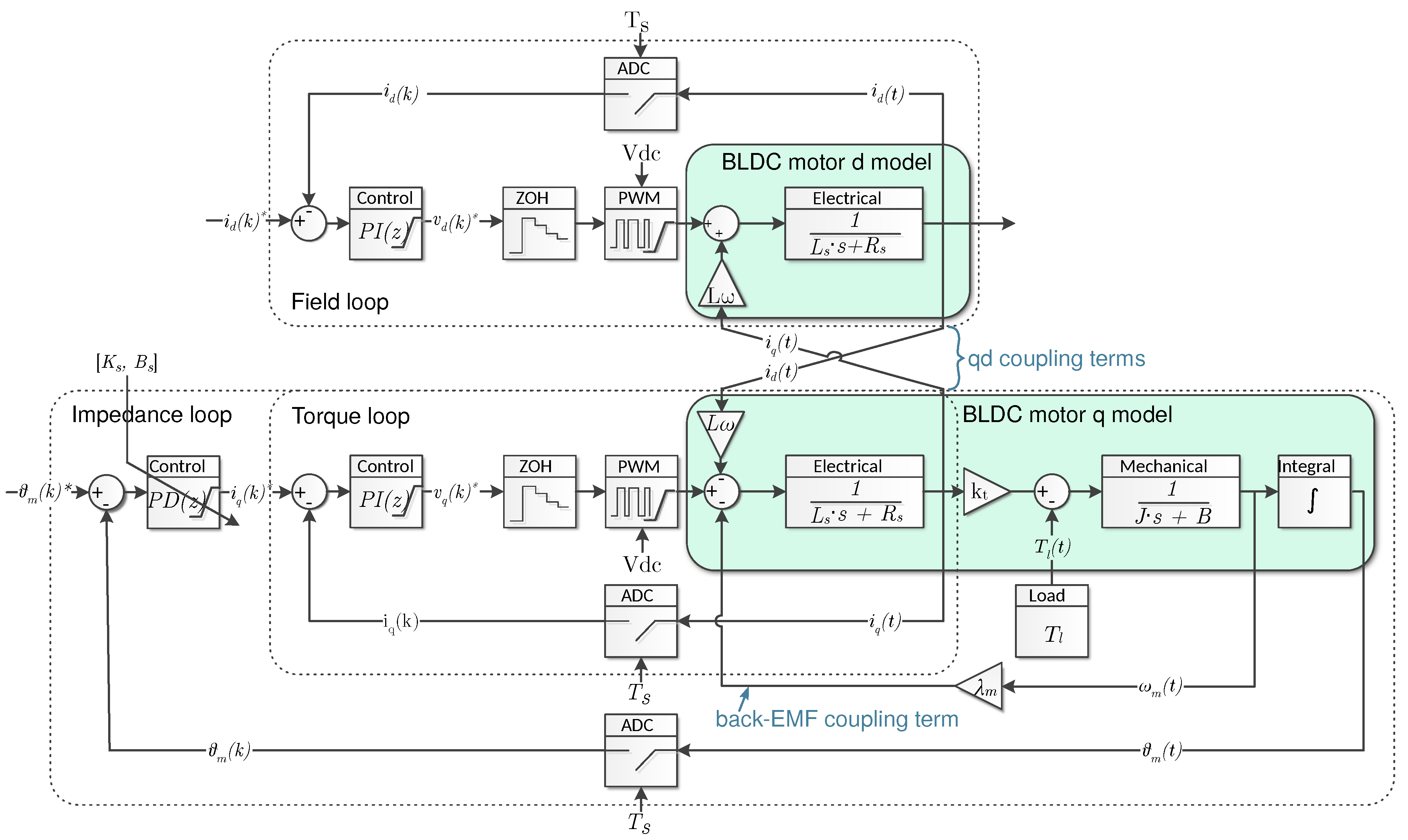
2. Proposed Active Impedance Controller System
3. Motor Controller Designs
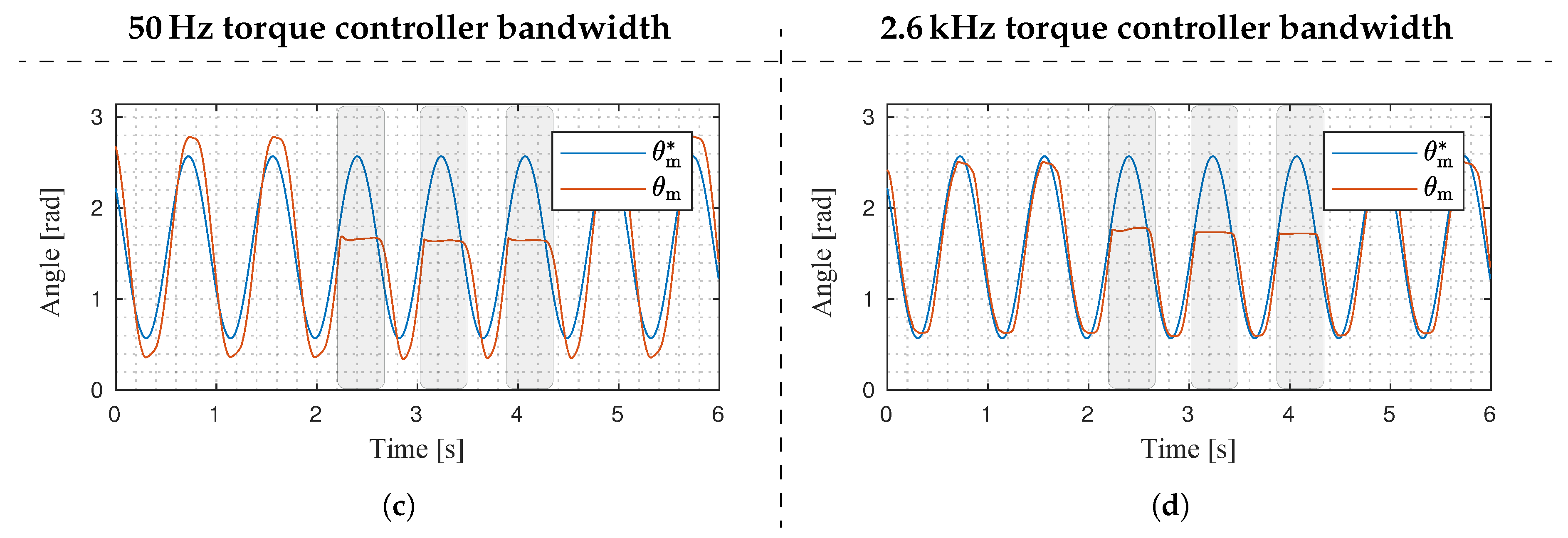
3.1. Torque and Field Controller Design
3.2. Active Impedance Controller Design
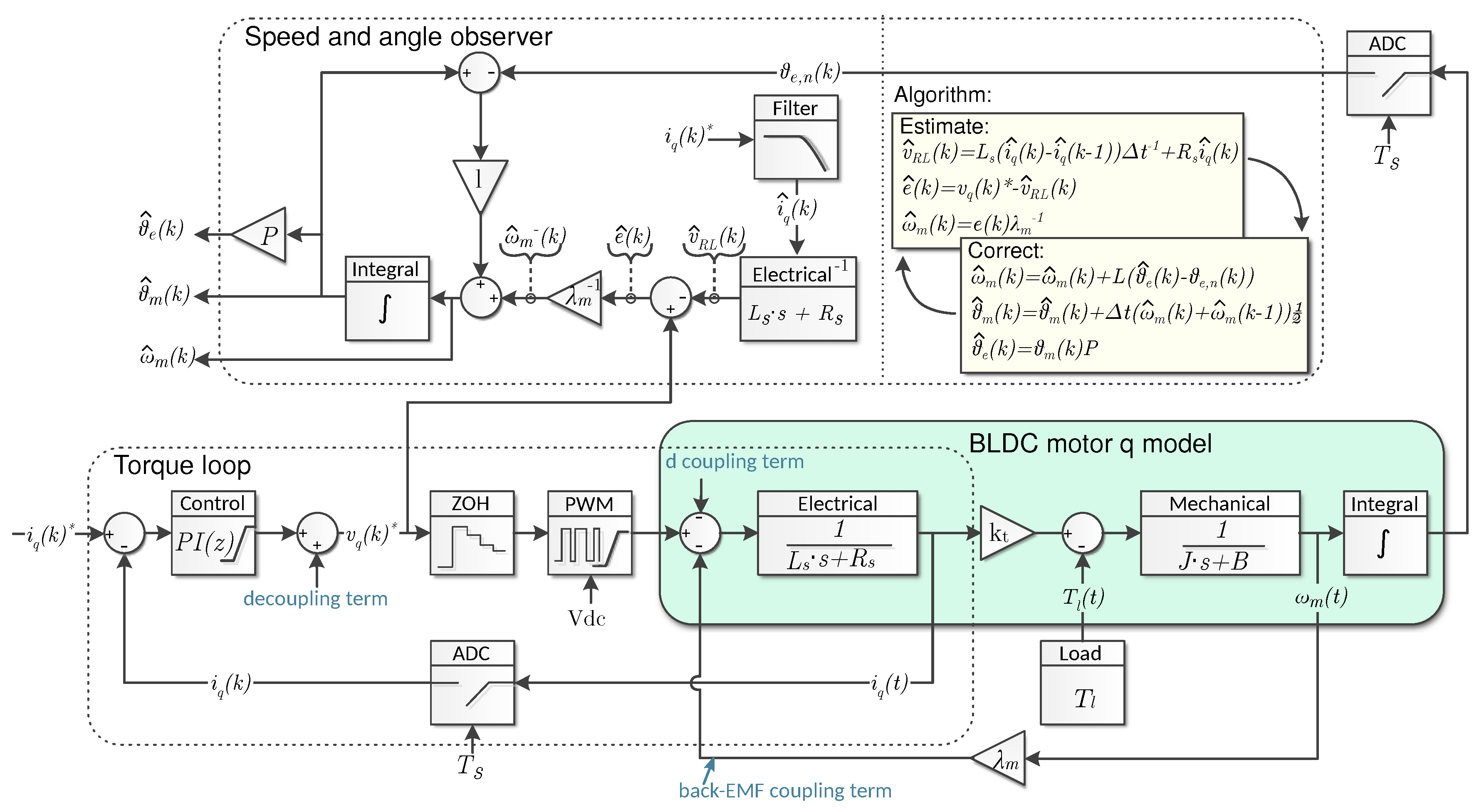
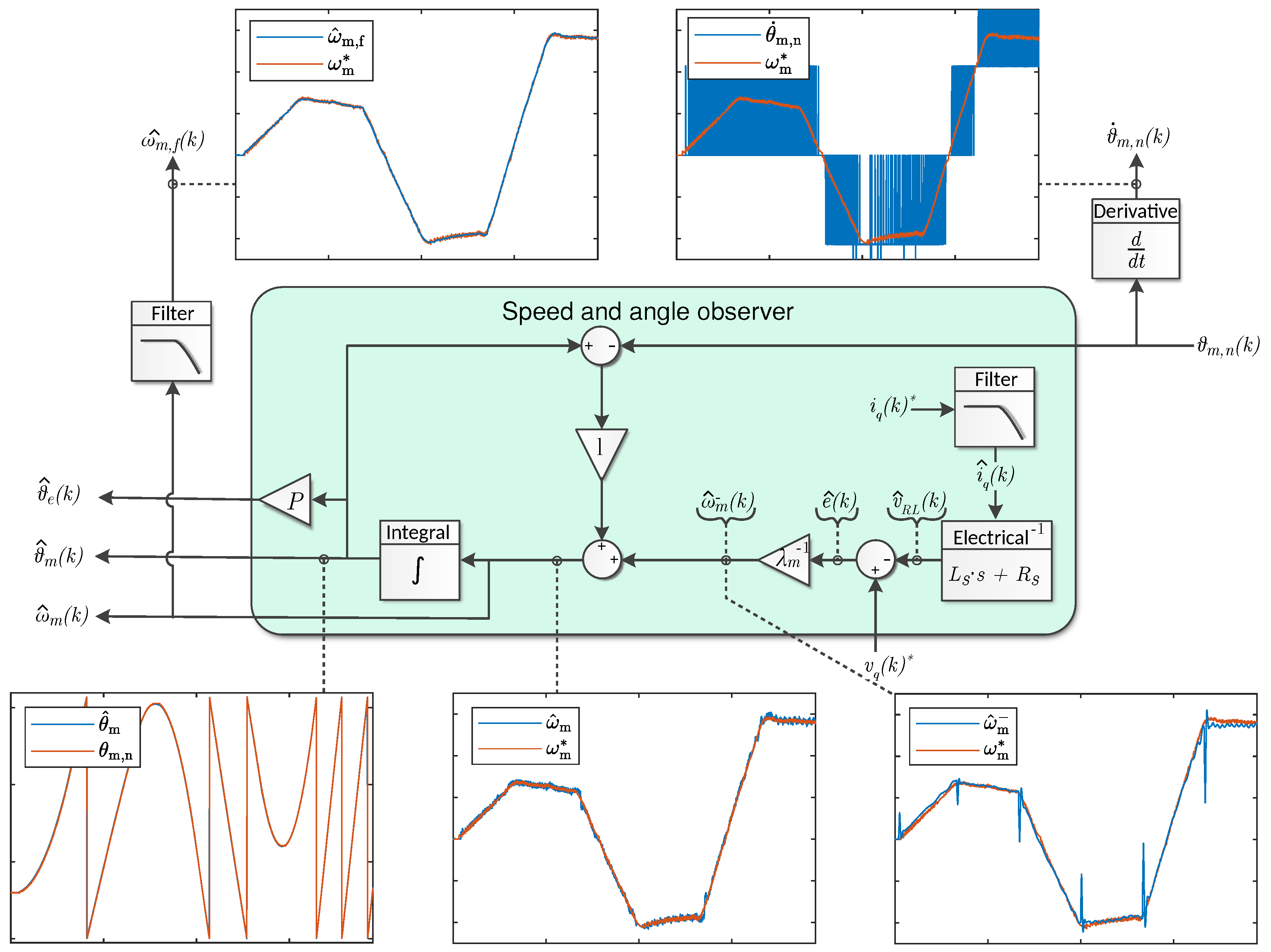
4. Novel Observer: Mechanical Angle, Electrical Angle and Speed Filtering
4.1. Estimation Step
4.2. Correction Step
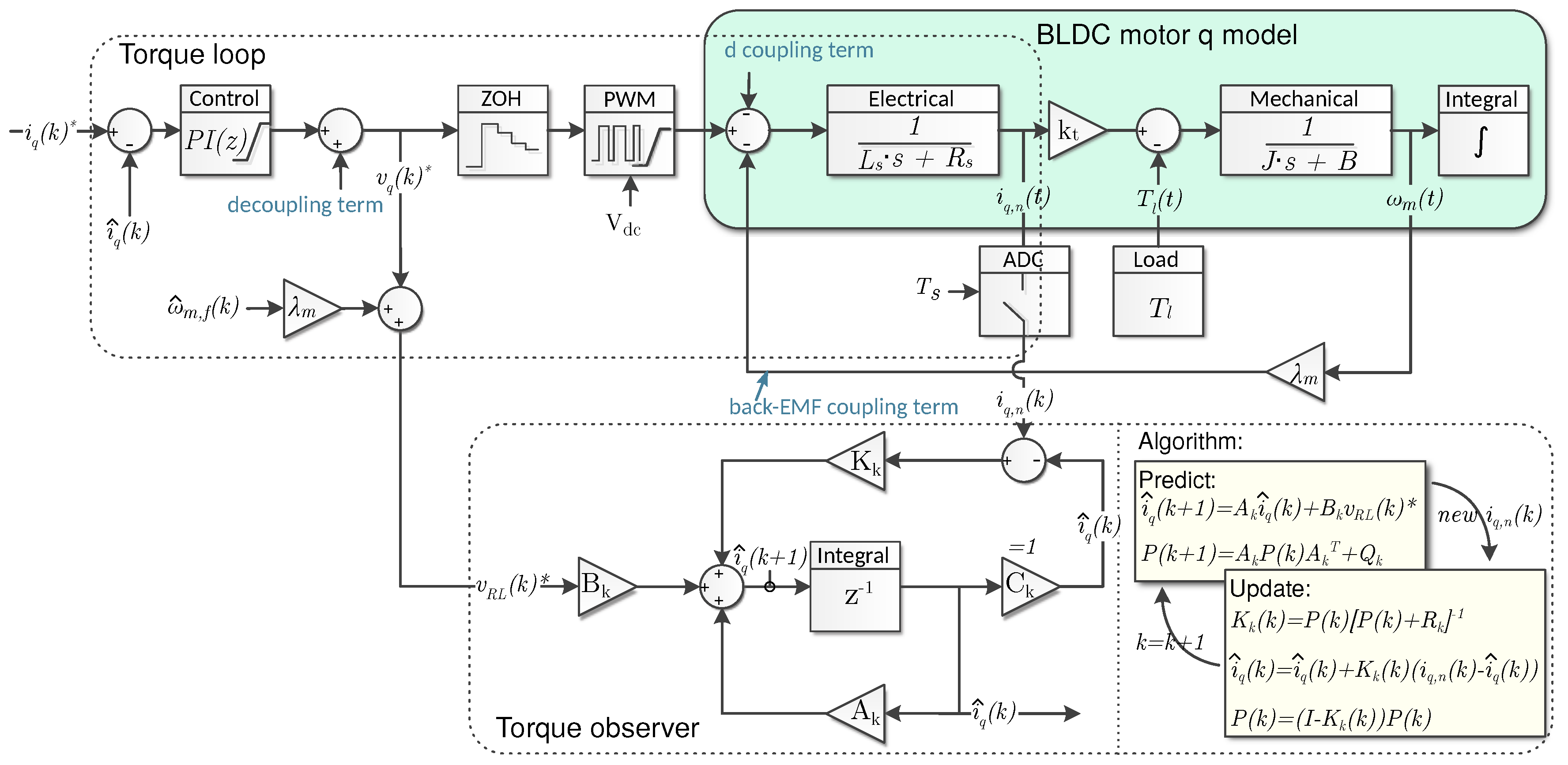
5. Kalman/Luenberger Observer: Quadrature Current Filtering
6. Experimental Test Setups
7. Experimental Results and Discussion
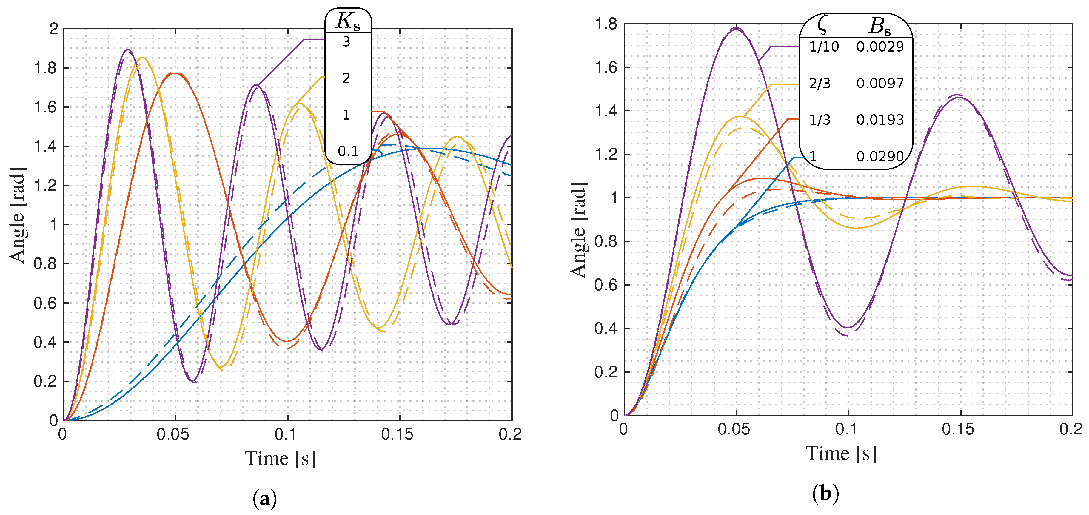
7.1. Experimental Results: Active Impedance Controller Compared with Dynamic Impedance Model
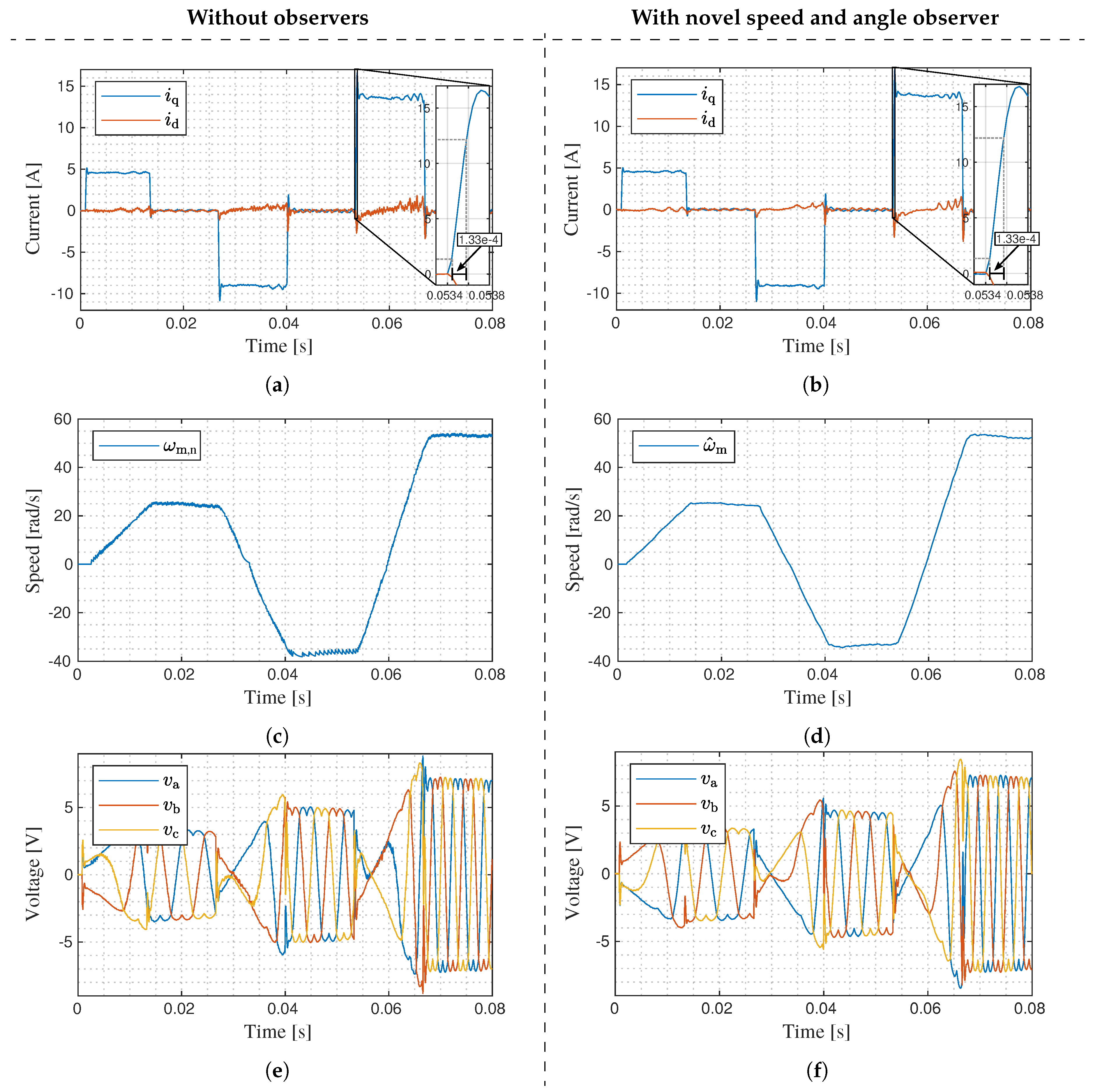
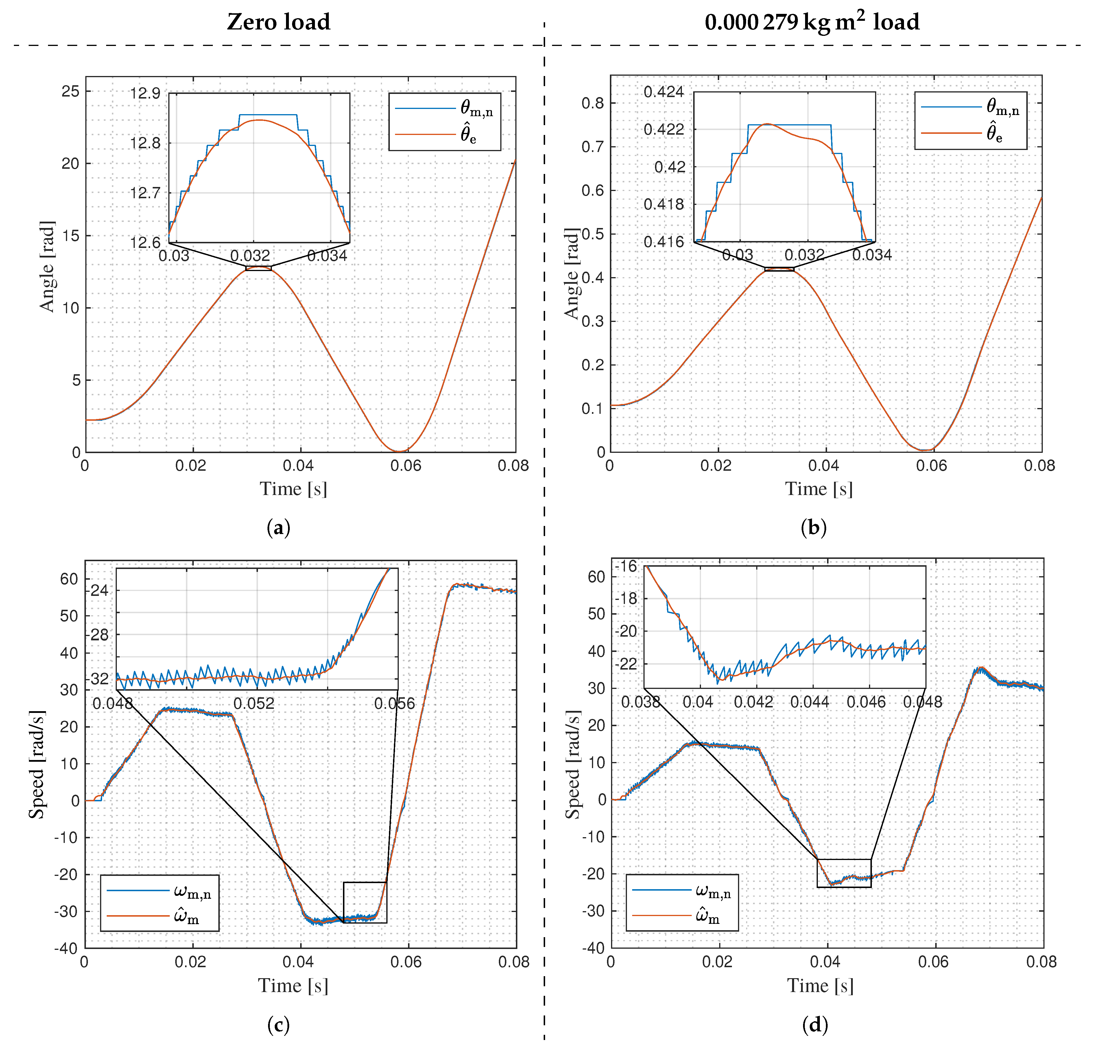
7.2. Experimental Results: Torque Control—Angle and Speed Observer vs. no Observer
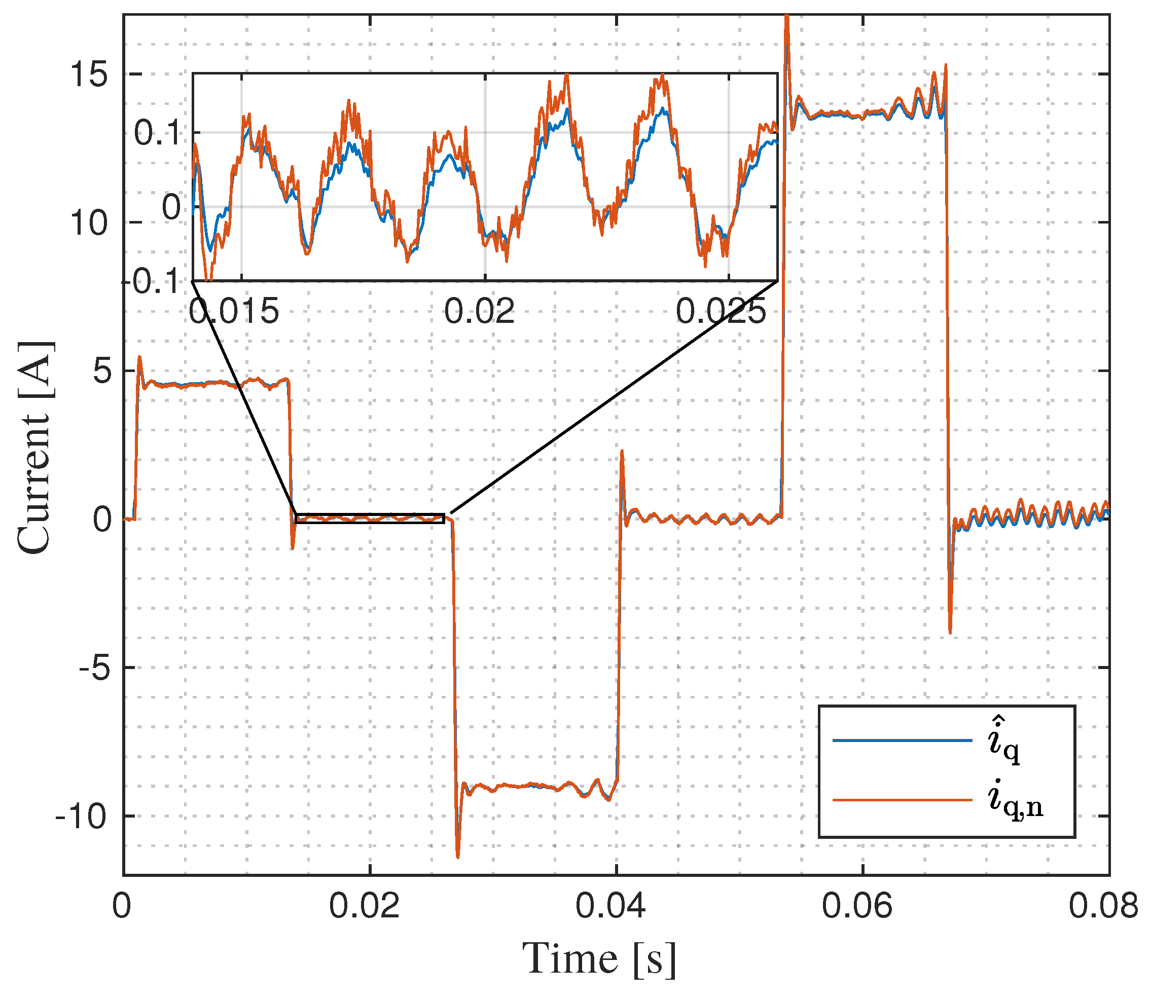
7.3. Experimental Results: Torque Control—Torque Observer vs. no Observers.
7.4. Experimental Results: Speed Control—Angle, Speed and Torque Observer vs. no Observers
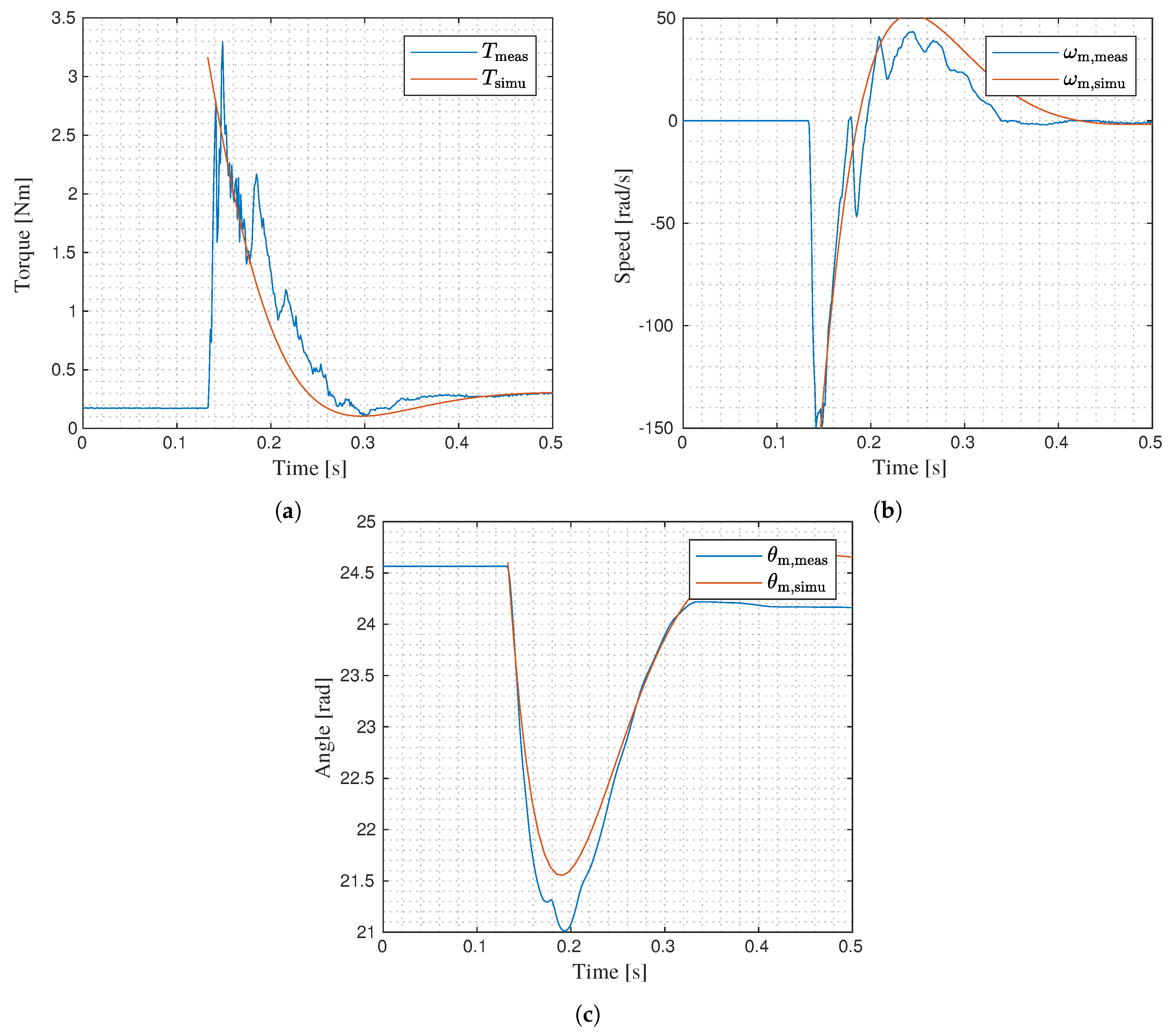
7.5. Experimental Results: Active Impedance Control with Angle/Speed and Torque Observers—Impact Force Load
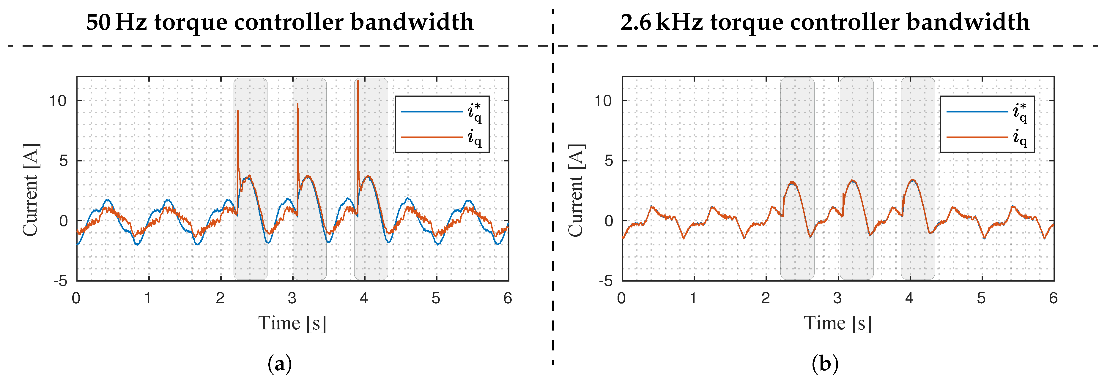
7.6. Experimental Results: Active Impedance Control with Angle/Speed and Torque Observers—Compliance Test
8. Conclusions
Supplementary Materials
- Video S1: 30 / speed step test without observers (0 load)
- Video S2: 30 / speed step test with observers (0 load)
- Video S3: 30 / speed step test without observers (3 load)
- Video S4: 30 / speed step test with observers (3 load)
- Video S5: Multi speed step test without observers 0 load)
- Video S6: Multi speed step test with observers 0 load)
- Video S7: Impact force test (stiff control)
- Video S8: Impact force test (soft control)
- Video S9: Active impedance control test without observers
- Video S10: Active impedance control test with observers
- Video S11: Human-robot collision test low bandwidth
- Video S12: Human-robot collision test high bandwidth
- C code S13: Entire motor controller source code
- PCB files S14: Motor Module 10S
Author Contributions
Funding
Acknowledgments
Conflicts of Interest
Appendix A. Clarke and Park Transformation
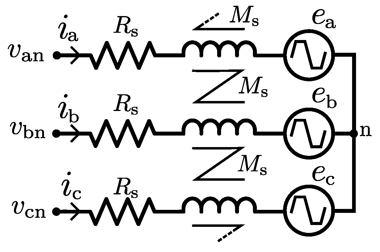
Appendix B. BLDC Motor Model in the Rotating Reference Frame

Appendix C. Controller Pseudo Algorithm
Appendix D. Specifications of the Test Configuration

| Description | Reference | Unit | Value |
|---|---|---|---|
| Internal Line Resistance | R | 95 | |
| Internal Line Inductance | L | ||
| Max Continuous Current @180 | 33 | ||
| Max Continuous Power @180 | |||
| Nominal Excitation Voltage | 40 | ||
| Peak Stall Torque | |||
| Max Operating Temperature | 180 | ||
| Dimensions | DxT | Ø89 × 40 | |
| Shaft Diameter | 15 | ||
| Weight | M | 500 | |
| Torque Constant | |||
| Velocity Constant | 80 | ||
| Number of poles | P | - | 40 |
| Moment of inertia on rotor | I | 2 | |
| Motor viscous damping | B | ||
| Torque controller proportional gain | |||
| Torque controller integrator gain | |||
| Speed controller proportional gain | |||
| Speed/Angle observer gain | l | 1500 | |
| Luenberger observer gain | |||
| Sampling/PWM period | 40 | ||
| Magnetic encoder resolution | - | bits | 12 |
Appendix E. Impedance Test Parameters
| Impedance Model Parameters | Impedance Controller Parameters | ||||
|---|---|---|---|---|---|
| # | Spring Constant | Damping Constant | Proportional Gain | Derivative Gain | Attenuation Factor |
| [] | [] | [] | [] | α | |
| Test 1 | |||||
| Test 2 | 1 | ||||
| Test 3 | 2 | ||||
| Test 4 | 3 | ||||
| Test 5 | 2 | ||||
| Test 6 | 2 | ||||
| Test 7 | 2 | ||||
| Test 8 | 2 | ||||
Appendix F. Impact Test Parameters
| Impedance Model Parameters | Impedance Controller Parameters | |||
|---|---|---|---|---|
| # | Spring Constant | Damping Constant | Proportional Gain | Derivative Gain |
| [] | [] | [] | [] | |
| Test 1 | ||||
Appendix G. Derivation of Torque and Field Controller Design Equations
Appendix H. Symbolic Expressions of the Sensitivity Factors
Appendix H.1. Direct and Quadrature Current with Respect to Measured Angle
Appendix H.2. Direct and Quadrature Current with Respect to Measured Currents
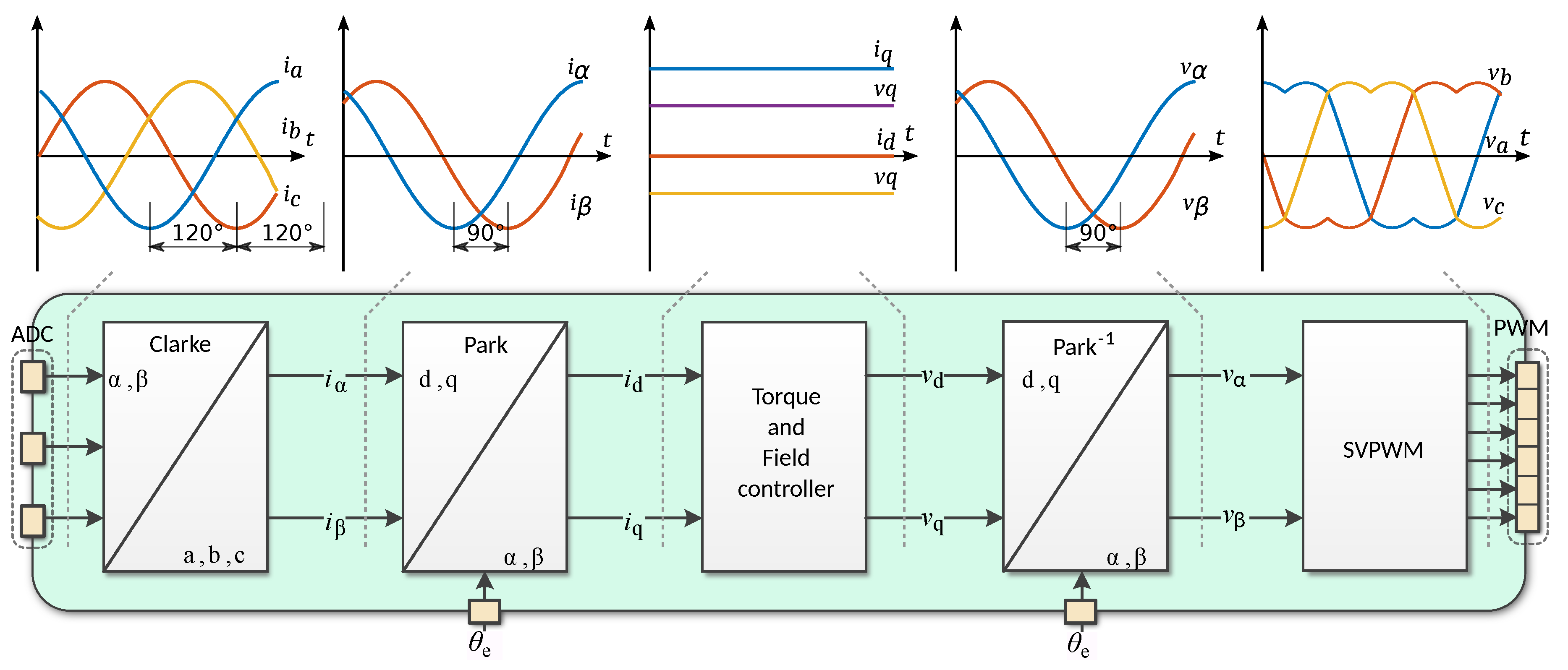
Appendix I. Field Oriented Control

Appendix J. Noise Analysis Based on the Sensitivity Method
- High-end and off-the-shelf magnetic encoders are typically maximum 12-bit resolution
- The direct current is highly affected by angle sensor noise
- The Proportional-Derivative (PD) controller amplifies angle sensor noise which is almost directly injected into the motor phases (due to high-bandwidth torque control)
- If speed feed-forward is required (to decouple the torque loop from the back-EMF), the angle sensor value is once again amplified and injected directly into the motor phases
Appendix K. Impact Force Benchmark Test Configuration

Appendix L. Electronics and Software Platform


References
- Wensing, P.M.; Wang, A.; Seok, S.; Otten, D.; Lang, J.; Kim, S. Proprioceptive actuator design in the MIT cheetah: Impact mitigation and high-bandwidth physical interaction for dynamic legged robots. IEEE Trans. Robot. 2017, 33, 509–522. [Google Scholar] [CrossRef]
- Vallery, H.; Veneman, J.; van Asseldonk, E.; Ekkelenkamp, R.; Buss, M.; van Der Kooij, H. Compliant actuation of rehabilitation robots. IEEE Robot. Autom. Mag. 2008, 15, 60–69. [Google Scholar] [CrossRef]
- Androwis, G.J.; Nolan, K.J. Evaluation of a Robotic Exoskeleton for Gait Training in Acute Stroke: A Case Study. In Wearable Robotics: Challenges and Trends; Springer: Cham, Switzerland, 2017; Volume 16, pp. 9–13. [Google Scholar] [CrossRef]
- Sharifi, M.; Salarieh, H.; Behzadipour, S.; Tavakoli, M. Biomedical Signal Processing and Control Beating-heart robotic surgery using bilateral impedance control: Theory and experiments. Biomed. Signal Process. Control 2018, 45, 256–266. [Google Scholar] [CrossRef]
- Williams, M.R.; Andrea, S.D.; Herr, H.M. Impact on gait biomechanics of using an active variable impedance prosthetic knee. J. NeuroEng. Rehabil. 2016, 13, 54. [Google Scholar] [CrossRef]
- Milwich, M.; Selvarayan, S.K.; Gresser, G.T. Fibrous materials and textiles for soft robotics. In Soft Robotics: Transferring Theory to Application; Springer: Berlin, Germany, 2015; p. 11. [Google Scholar] [CrossRef]
- Gracia, L.; Perez-vidal, C.; Valls-miro, J. Advanced Mathematical Methods for Collaborative Robotics. Math. Probl. Eng. 2018, 2018, 10–13. [Google Scholar] [CrossRef]
- Beltran-Carbajal, F.; Valderrabano-Gonzalez, A.; Favela-Contreras, A.; Hernandez-Avila, J.L.; Lopez-Garcia, I.; Tapia-Olvera, R. An Active Vehicle Suspension Control Approach with Electromagnetic and Hydraulic Actuators. Actuators 2019, 8, 35. [Google Scholar] [CrossRef]
- Vanderborght, B.; Albu-schaeffer, A.; Bicchi, A.; Burdet, E.; Caldwell, D.G. Variable impedance actuators: A review. Robot. Autonomous Syst. 2013, 61, 1601–1614. [Google Scholar] [CrossRef]
- Boaventura, T.; Medrano-Cerda, G.A.; Semini, C.; Buchli, J.; Caldwell, D.G. Stability and performance of the compliance controller of the quadruped robot HyQ. In Proceedings of the IEEE International Conference on Intelligent Robots and Systems, Tokyo, Japan, 3–7 November 2013; pp. 1458–1464. [Google Scholar] [CrossRef]
- Roozing, W.; Malzahn, J.; Kashiri, N.; Caldwell, D.G.; Tsagarakis, N.G. On the Stiffness Selection for Torque-Controlled Series-Elastic Actuators. IEEE Robot. Autom. Lett. 2017, 2, 2255–2262. [Google Scholar] [CrossRef]
- Katz, B.G. A Low Cost Modular Actuator for Dynamic Robots. Master’s Thesis, Massachusetts Institute of Technology, Cambridge, MA, USA, 2018. [Google Scholar]
- Bhatia, A.; Johnson, A.M.; Mason, M.T. Direct Drive Hands: Force-Motion Transparency in Gripper Design. In Proceedings of the Robotics: Science and Systems, Freiburg, Germany, 22–26 June 2019. [Google Scholar]
- Verstraten, T.; Beckerle, P.; Furnémont, R.; Mathijssen, G. Series and Parallel Elastic Actuation: Impact of natural dynamics on power and energy consumption. MAMT 2016, 102, 232–246. [Google Scholar] [CrossRef]
- Hogan, N. Impedance Control: An Approach to Manipulation. In Proceedings of the 1984 American Control Conference, San Diego, CA, USA, 6–8 June 1984; pp. 304–313. [Google Scholar] [CrossRef]
- Semini, C.; Barasuol, V.; Boaventura, T.; Frigerio, M.; Focchi, M.; Caldwell, D.G.; Buchli, J. Towards versatile legged robots through active impedance control. Int. J. Robot. Res. 2015, 34, 1003–1020. [Google Scholar] [CrossRef]
- Gabriel, R.; Leonhard, W.; Nordby, C.J. Field-Oriented Control of a Standard AC Motor Using Microprocessors. IEEE Trans. Ind. Appl. 1980, IA-16, 186–192. [Google Scholar] [CrossRef]
- Schindlbeck, C.; Haddadin, S. Unified Passivity-Based Cartesian Force/Impedance Control for Rigid and Flexible Joint Robots via Task-Energy Tanks. In Proceedings of the 2015 IEEE International Conference on Robotics and Automation (ICRA), Seattle, WA, USA, 26–30 May 2015; pp. 440–447. [Google Scholar] [CrossRef]
- Niccol, L.R.; Molinari, L. Discrete-Time Formulation for Optimal Impact Control in Interaction Tasks. J. Intell. Robot. Syst. 2018, 90, 407–417. [Google Scholar]
- Cherubini, A.; Passama, R.; Crosnier, A.; Lasnier, A.; Fraisse, P. Robotics and Computer-Integrated Manufacturing Collaborative manufacturing with physical human—Robot interaction. Robot. Comput. Integr. Manuf. 2016, 40, 1–13. [Google Scholar] [CrossRef]
- Roveda, L. A User-Intention Based Adaptive Manual Guidance with Force-Tracking Capabilities Applied to Walk-Through Programming for Industrial Robots. In Proceedings of the 2018 15th International Conference on Ubiquitous Robots (UR), Honolulu, HI, USA, 26–30 June 2018; pp. 369–376. [Google Scholar] [CrossRef]
- Roveda, L. Adaptive Interaction Controller for Compliant Robot Base Applications. IEEE Access 2019, 7, 6553–6561. [Google Scholar] [CrossRef]
- Kim, S.H. Sensorless technique using the motor model. In Electric Motor Control: DC, AC, and BLDC Motors; Elsevier Science: Amsterdam, The Netherlands, 2017. [Google Scholar]
- Kshirsagar, P.; Burgos, R.P.; Jang, J.; Lidozzi, A.; Wang, F.; Boroyevich, D.; Sul, S.K. Implementation and sensorless vector-control design and tuning strategy for SMPM machines in fan-type applications. IEEE Trans. Ind. Appl. 2012, 48, 2402–2413. [Google Scholar] [CrossRef]
- Chi, S.; Zhang, Z.; Xu, L. Sliding-mode sensorless control of direct-drive PM synchronous motors for washing machine applications. IEEE Trans. Ind. Appl. 2009, 45, 582–590. [Google Scholar] [CrossRef]
- Kim, S.H. Vector Control of Permanent Magnet Synchronous Motors. In Electric Motor Control: DC, AC, and BLDC Motors; Chapter 5.5; Elsevier Science: Amsterdam, The Netherlands, 2017. [Google Scholar]
- Mon-Nzongo, D.L.; Jin, T.; Ekemb, G.; Bitjoka, L. Decoupling Network of Field-Oriented Control in Variable-Frequency Drives. IEEE Trans. Ind. Electron. 2017, 64, 5746–5750. [Google Scholar] [CrossRef]
- Hyun, D.J.; Seok, S.; Lee, J.; Kim, S. High speed trot-running: Implementation of a hierarchical controller using proprioceptive impedance control on the MIT Cheetah. Int. J. Robot. Res. 2014, 33, 1417–1445. [Google Scholar] [CrossRef]
- Luenberger, D. Introduction To Observers. IEEE Trans. Autom. Control 1971, AC16, 596–602. [Google Scholar] [CrossRef]
- Kalman, R.E. A New Approach to Linear Filtering and Prediction Problems. J. Basic Eng. 2011, 82, 35. [Google Scholar] [CrossRef]
- Horváth, Z.; Molnárka, G. Design Luenberger Observer for an Electromechanical Actuator. Acta Technica Jaurinensis 2014, 7, 328–343. [Google Scholar] [CrossRef][Green Version]
- Alessandri, A.; Coletta, P. Design of Luenberger Observers for a Class of Hybrid Linear Systems. In Proceedings of the International Workshop on Hybrid Systems: Computation and Control (HSCC 2001), Rome, Italy, 28–30 March 2001; pp. 7–18. [Google Scholar] [CrossRef]
- Li, M.; Kang, R.; Branson, D.T.; Dai, J.S. Model-Free Control for Continuum Robots Based on an Adaptive Kalman Filter. IEEE/ASME Trans. Mechatron. 2018, 23, 286–297. [Google Scholar] [CrossRef]
- Schulz, M.W.; Clarke, E. Determination of Instantaneous Currents and Voltages by Means of Alpha, Beta, and Zero Components. Trans. Am. Inst. Electr. Eng. 1951, 70, 1248–1255. [Google Scholar]
- Park, R.H. Two Reaction Theory of Synchronous Machines Generalized Method of Analysis-Part I. Trans. Am. Inst. Electr. Eng. 1929, 48, 716–727. [Google Scholar] [CrossRef]
- Lazor, M.; Stulrajter, M. Modified field oriented control for smooth torque operation of a BLDC motor. In Proceedings of the 10th International Conference, ELEKTRO 2014, Žilina, Slovakia, 19–20 May 2014; pp. 180–185. [Google Scholar] [CrossRef]
- Kshirsagar, P.; Krishnan, R. High-efficiency current excitation strategy for variable-speed nonsinusoidal back-EMF PMSM machines. IEEE Trans. Ind. Appl. 2012, 48, 1875–1889. [Google Scholar] [CrossRef]
- Oliveira, A.A.; De Monteiro, J.R.; Aguiar, M.L.; Gonzaga, D.P. Extended DQ transformation for vectorial control applications of non-sinusoidal permanent magnet synchronous machines. In Proceedings of the PESC Record—2005 IEEE 36th Power Electronics Specialists Conference, Recife, Brazil, 16 June 2005; pp. 1807–1812. [Google Scholar] [CrossRef]
- Kumar, M.; Singh, B.; Singh, B.P. Modeling and Simulation of Permanent Magnet Brushless Motor Drives using Simulink. In Proceedings of the National Power Systems Conference, Kharagpur, India, 27–29 December 2002; Volume 1, pp. 253–258. [Google Scholar]
- Saltelli, A. Sensitivity Analysis for Importance Assessment—Risk Analysis. Risk Anal. 2002, 22, 579–590. [Google Scholar] [CrossRef]
- Saltelli, A.; Ratto, M.; Andres, T.; Campolongo, F.; Cariboni, J.; Gatelli, D.; Saisana, M.; Tarantola, S. Methods and Settings for Sensitivity Analysis—An Introduction; Global Sensitivity Analysis—The Primer, John Wiley & Sons, Ltd.: Chichester, UK, 2002; Chapter 1.2; Volume 52. [Google Scholar]

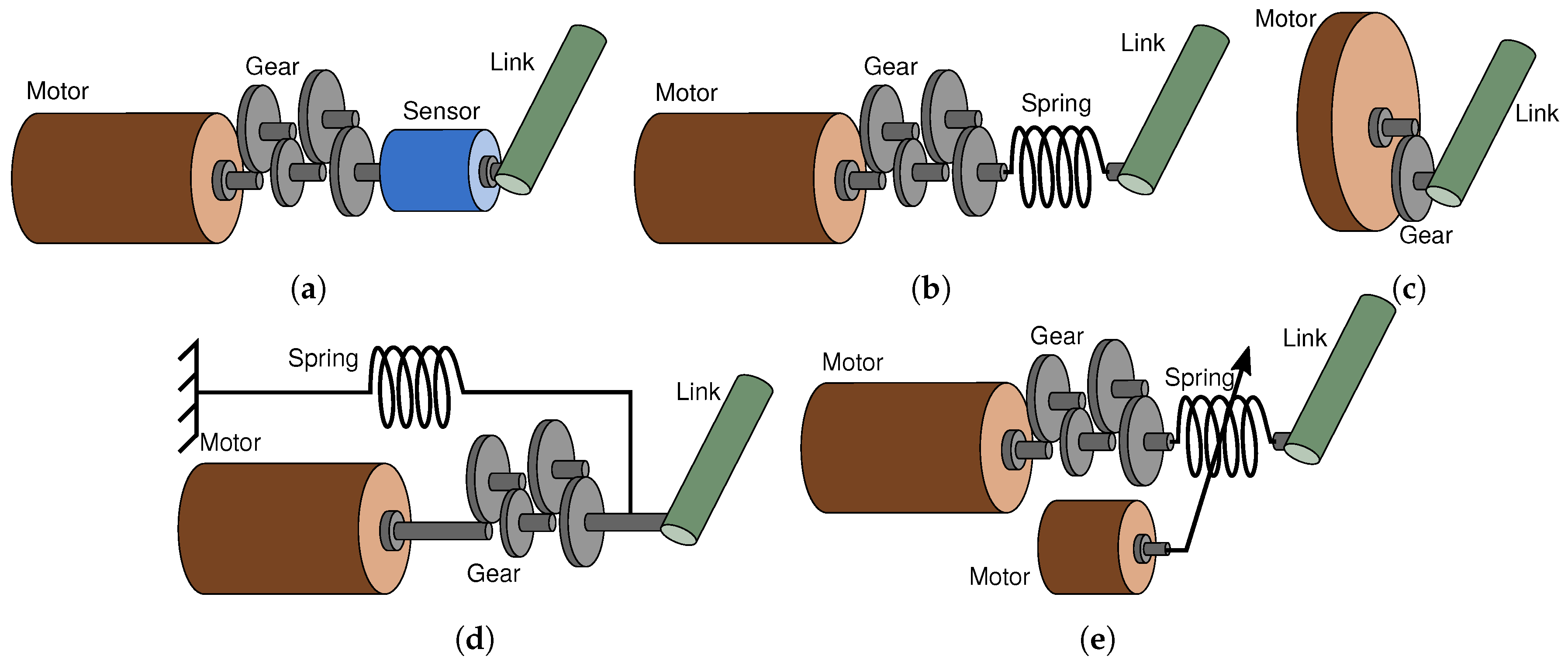
- (a)
- Geared Motor with Force/Torque sensor (GMS) embeds a low-diameter motor and a high gear ratio transmission to actuate the robot link. A torque or force sensor is used as feedback to perform torque or force control. Pros:variable impedance response, high torque density. Cons: sample delay (cannot mitigate high speed shocks), low open-loop force controller bandwidth (at end-effector), low Z-width [10], low force transparency.
- (b)
- Series Elastic Actuator (SEA) includes a low-diameter motor and a high gear ratio transmission to actuate the robot link. A spring is connected between the gears and the end-effector of the robot link. Pros: high torque density, high energy efficiency, simple control, no sample delay* (can mitigate high speed shocks). Cons: fixed impedance response [9], it offers improved force transparency and open-loop force controller bandwidth (at end-effector) in relation to GMS and PEA [11], but is not comparable to the proprioceptive actuator design on this matter [1,9,12,13].
- (c)
- Proprioceptive actuator includes a high-diameter motor and a low gear ratio transmission to actuate the robot link. As the transparency between the motor shaft and the end-effector is very low (due to low gearing and high stiffness), the motor phase currents can be used to estimate the torque at the end-effector (proprioception). Pros: high open-loop force controller bandwidth (at end-effector), high force transparency [1,9,12,13], high Z-width [10]. Cons: complex control, sample delay* (cannot mitigate high speed shocks), lower energy efficiency and torque density than other electromagnetic actuators [1].
- (d)
- Parallel Elastic Actuator (PEA) includes a low-diameter motor and a high gear ratio transmission to actuate the robot link. Additionally, it includes a spring which is connected in parallel with the robot link. Pros: high torque density, high efficiency [14], simple control, no sample delay* (can mitigate high speed shocks). Cons: fixed impedance response, low open-loop force controller bandwidth (at end-effector), low force transparency.
- (e)
- Variable Stiffness Actuator (VSA) is typically comprised of the same elements as SEA, where an additional motor is controlling the stiffness of the elastic element. Pros: high torque density, high energy efficiency [14], variable impedance response, no sample delay* (can mitigate high speed shocks). Cons: complex control, low open-loop force controller bandwidth (at end-effector), low force transparency.


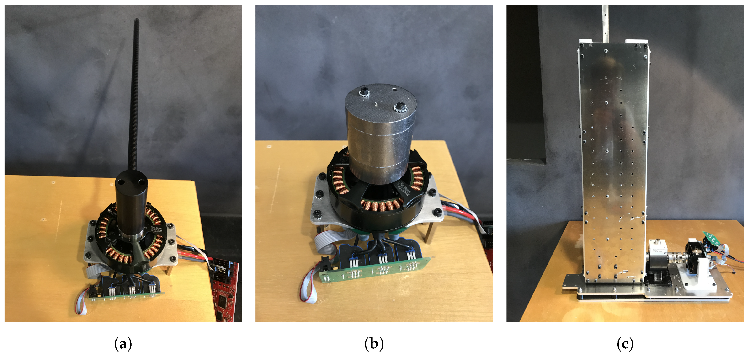
- (a)
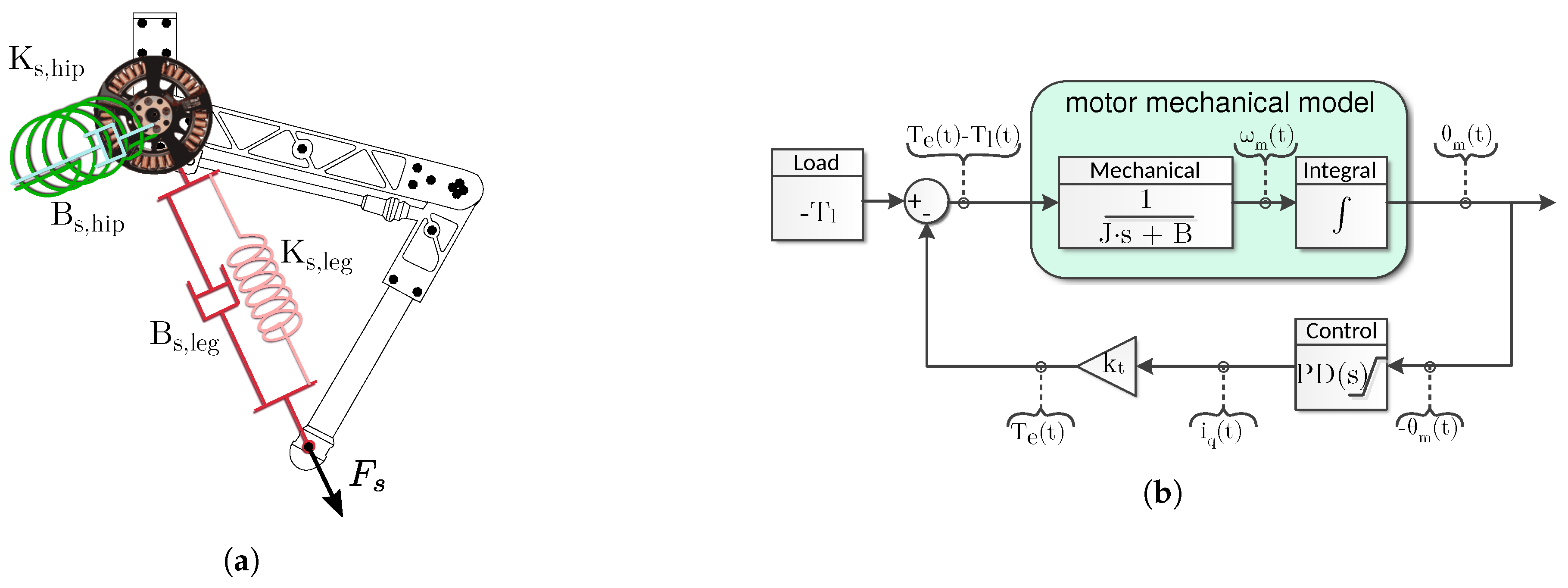
- 1-link load includes a 30 carbon fiber tube (propeller) attached to the motor shaft through a hollow cylindric plastic spacer. The purpose of this configuration is to demonstrate active impedance by applying external force to the propeller
- (b)
- Inertia load includes a 900 cylindric iron load directly attached to the motor shaft. The purpose of this setup is to demonstrate the proposed controller including a fixed level of attached inertia.
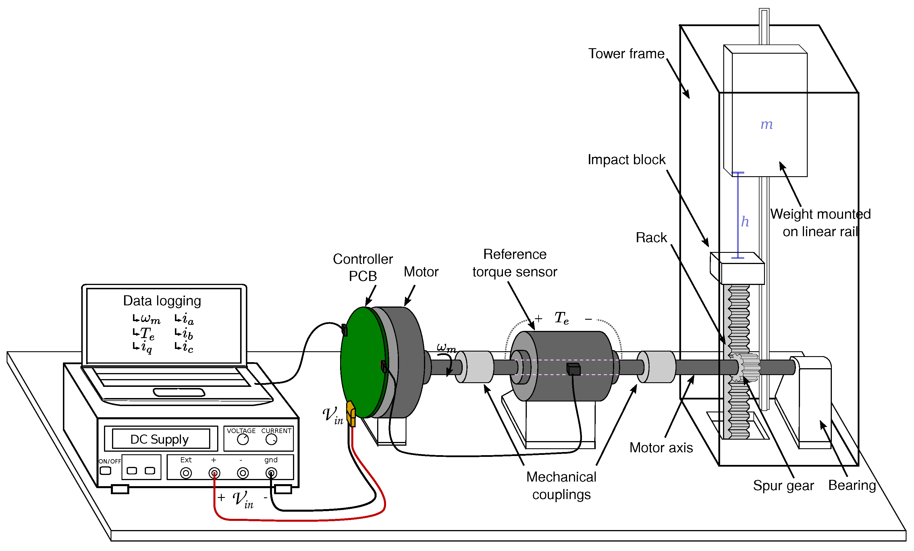
- (c)
- Impact load includes a weight which is mounted on a linear rail. The motor is connected to another rail through a torque sensor (T22/20NM), two mechanical couplings and a spur gear. The purpose of this setup is to demonstrate how the motor controller complies during impact force.


© 2019 by the authors. Licensee MDPI, Basel, Switzerland. This article is an open access article distributed under the terms and conditions of the Creative Commons Attribution (CC BY) license (http://creativecommons.org/licenses/by/4.0/).
Share and Cite
Lund, S.H.J.; Billeschou, P.; Larsen, L.B. High-Bandwidth Active Impedance Control of the Proprioceptive Actuator Design in Dynamic Compliant Robotics. Actuators 2019, 8, 71. https://doi.org/10.3390/act8040071
Lund SHJ, Billeschou P, Larsen LB. High-Bandwidth Active Impedance Control of the Proprioceptive Actuator Design in Dynamic Compliant Robotics. Actuators. 2019; 8(4):71. https://doi.org/10.3390/act8040071
Chicago/Turabian StyleLund, Simon Hjorth Jessing, Peter Billeschou, and Leon Bonde Larsen. 2019. "High-Bandwidth Active Impedance Control of the Proprioceptive Actuator Design in Dynamic Compliant Robotics" Actuators 8, no. 4: 71. https://doi.org/10.3390/act8040071
APA StyleLund, S. H. J., Billeschou, P., & Larsen, L. B. (2019). High-Bandwidth Active Impedance Control of the Proprioceptive Actuator Design in Dynamic Compliant Robotics. Actuators, 8(4), 71. https://doi.org/10.3390/act8040071