Abstract
The focus of this study lies on the investigation of the space vector modulation of a self-sensing three-phase radial active magnetic bearing. The determination of the rotor position information is performed by a current slope-based inductance measurement of the actuator coils. Therefore, a special pulse width modulation sequence is applied to the actuator coils by a conventional three-phase inverter. The choice of the modulation type is not unique and provides degrees of freedom for different modulation patterns, which are described in this work. For a self-sensing operation of the bearing, certain constraints of the space vector modulation must be considered. The approach of a variable space vector modulation is investigated to ensure sufficient dynamic in the current control as well as the suitability for a self-sensing operation with an accurate rotor position acquisition. Therefore, different space vector modulation strategies are considered in theory as well as proven in experiments on a radial magnetic bearing prototype. Finally, the performance of the self-sensing space vector modulation method is verified by an external position measurement system.
1. Introduction
Magnetic bearings are of great significance for the stabilization of levitating rotors. Due to the fact that it is impossible to stabilize all degrees of freedom of a rigid body by permanent magnets, a force of a different physical origin must be applied for rotor stabilization [1,2]. Therefore, the rotor can be stabilized by electromagnets, which is stated as active magnetic bearing (AMB). AMBs require a position feedback information of the rotor to allow a stable operation. In this work, a self-sensing method is used to obtain the rotor position instead of using separate position sensors. The operation of self-sensing AMBs has been a field of research for many years [3,4,5] and provides advantages concerning sensor failure, construction space and production costs of the AMB. The self-sensing position determination of this study is performed by a modulation-based current switching ripple evaluation of the actuator coils. Previous studies presented different approaches for extracting the rotor position information out of the current ripple, such as current slope measurements [6,7], current ripple demodulation [8] or by the usage of artificial neural networks [9]. In this proposal, the so-called INFORM (Indirect Flux Detection by Online Reactance Measurement) method is used to determine the rotor position. This method was originally designed for the rotor angle determination of a permanent magnet synchronous motor [10]. Concerning AMBs, the INFORM method is based on a current slope measurement, detecting the inductance change depending on the rotor’s eccentricity. As previously described in [11], the implementation of the self-sensing operation was based on an injection of voltage pulses to the actuator coils. Therefore, the current controller stops in equidistant time steps and measurement pulses are applied to the coils. This approach has the drawback of a limited bandwidth of the position measurement and an interruption of the current controller. To avoid this circumstance, the required pulse pattern for position measurement is embedded in the pulse width modulation (PWM) sequence of the current controller. The use of an embedded pulse pattern, in particular the 3-Active pattern [12], is the point of origin for the space vector modulation in this work.
2. Self-Sensing Bearing Setup
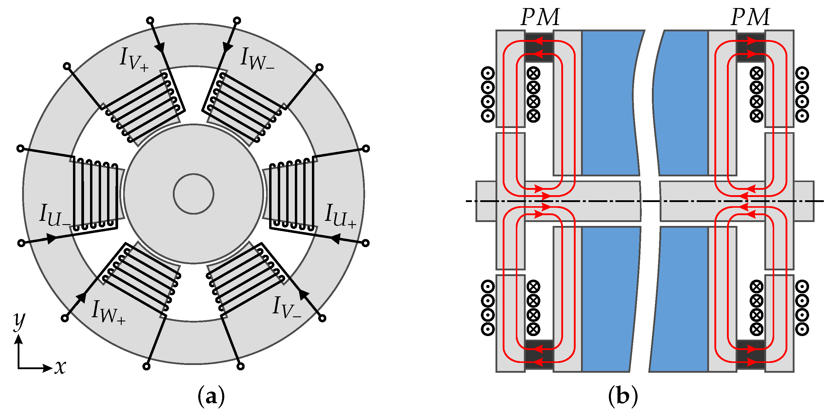
The bearing setup consists of two radial homopolar six pole AMBs with a common shaft as illustrated in Figure 1. The bias flux of the bearing is realized by the use of permanent magnets (PM). An axial displacement of the rotor is stabilized by a positive axial stiffness given by the bias flux and the geometry of the bearing (Figure 1b).
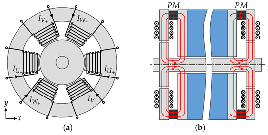
Figure 1.
(a) Structural design of the six pole radial homopolar active magnetic bearing. (b) Cross section of the shaft: The bias flux (indicated by red lines) is generated by means of permanent magnets.
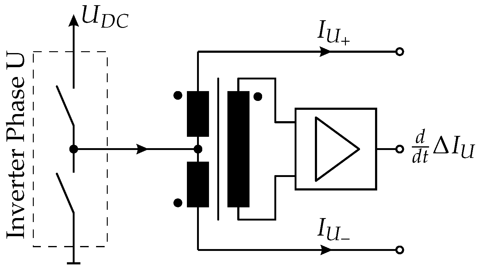
The stabilization of a radial rotor eccentricity is performed by the coils, which are driven in a differential configuration. The coils of the poles , , and the opposite coils are connected in wye-configuration. For achieving low system costs, a conventional three-phase inverter is aspired for the control of the AMB [13,14]. Two opposite coils are corresponding to one phase, which enables the use of a three-phase inverter. Figure 2 shows a differential transformer at the connection point of the positive and negative phase of the bearing.

Figure 2.
Differential current slope measurement by means of a differential open loop transformer.
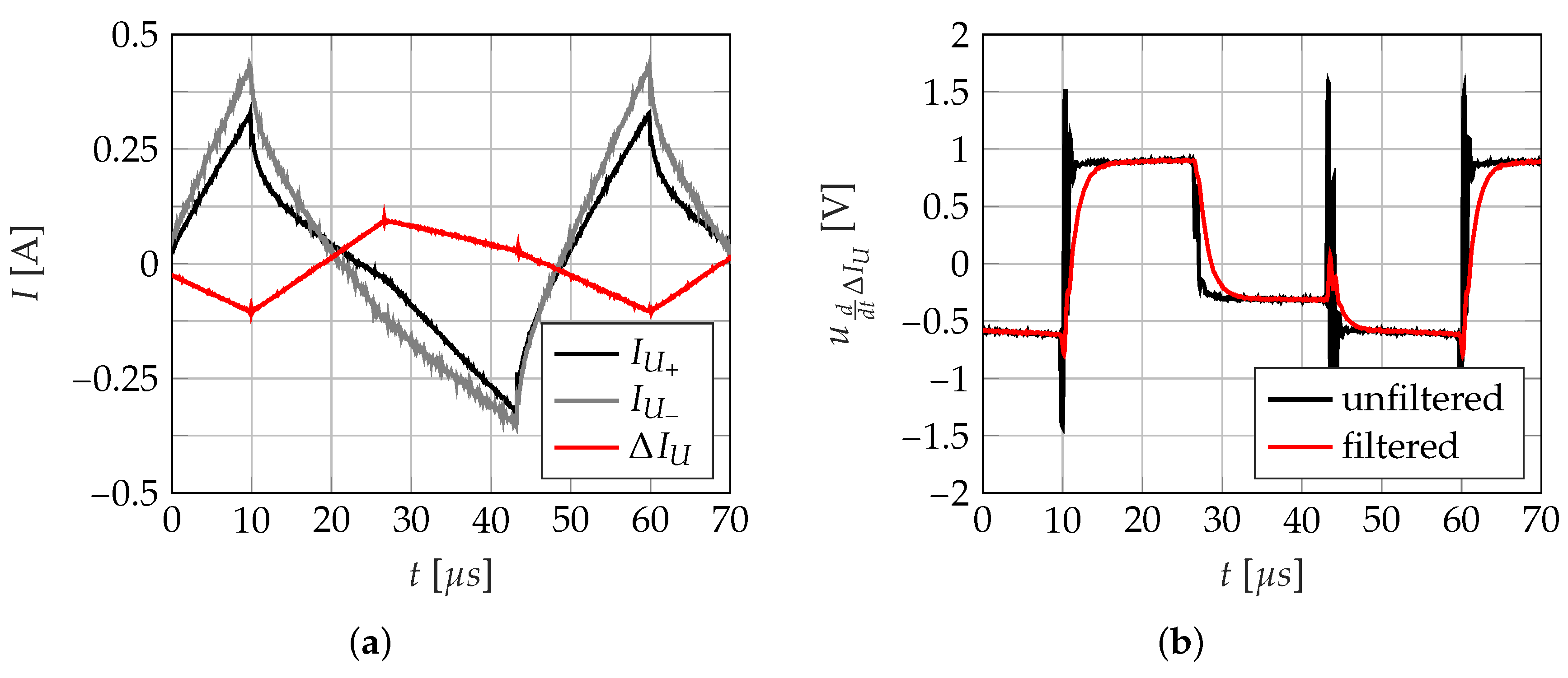
By the usage of an open loop transformer in each phase, it is possible to connect the AMB to a three-phase inverter. The transformer can be realized as a separate unit or also be integrated in the printed circuit board (PCB) of the power electronics [15]. The transformer output provides the differential current slope signal, which is required for the self-sensing operation of the bearing. Figure 3a shows the current ripple caused by the PWM switching pattern. Although the stator and the rotor components were built from laminated iron sheets, it can be seen that the current slope is distorted by eddy currents. To overcome this problem, the current slope measurement is performed as a differential evaluation of two opposite coils to suppress the influence of eddy currents. The differential current slope evaluation is not limited to the homopolar design and can be also applied to heteropolar bearings [16]. Another approach would be a model -based consideration of the eddy currents as shown in [17]. Figure 3b shows the output voltage of the open loop transformer corresponding to the differential current of Figure 3a. After the settling time, the output voltage is proportional to the differential current slope .
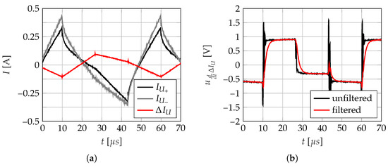
Figure 3.
(a) Current ripple of the actuator coils. The influence of eddy currents is mostly suppressed in the differential current signal (, ). (b) Output signal of the open loop transformer corresponding to (a). The output voltage is proportional to the differential current slope.
Thus, the rotor position can be obtained by the approximation
with the coil voltage and the position-depending inductance , which is described in [12].
3. Problem Formulation
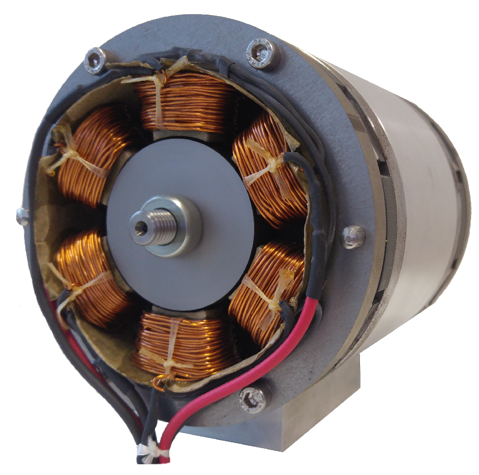
Measurements on a prototype of a self-sensing radial AMB (Figure 4) have shown significant power losses in the bearing in the 3-Active PWM mode. Consequently, the power losses lead to a temperature rise in the bearing, which is undesirable in many applications.
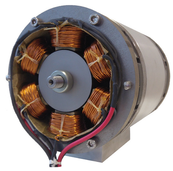
Figure 4.
Prototype of a self-sensing radial homopolar active magnetic bearing with six poles. The bias flux of the bearing is realized by the use of permanent magnets.
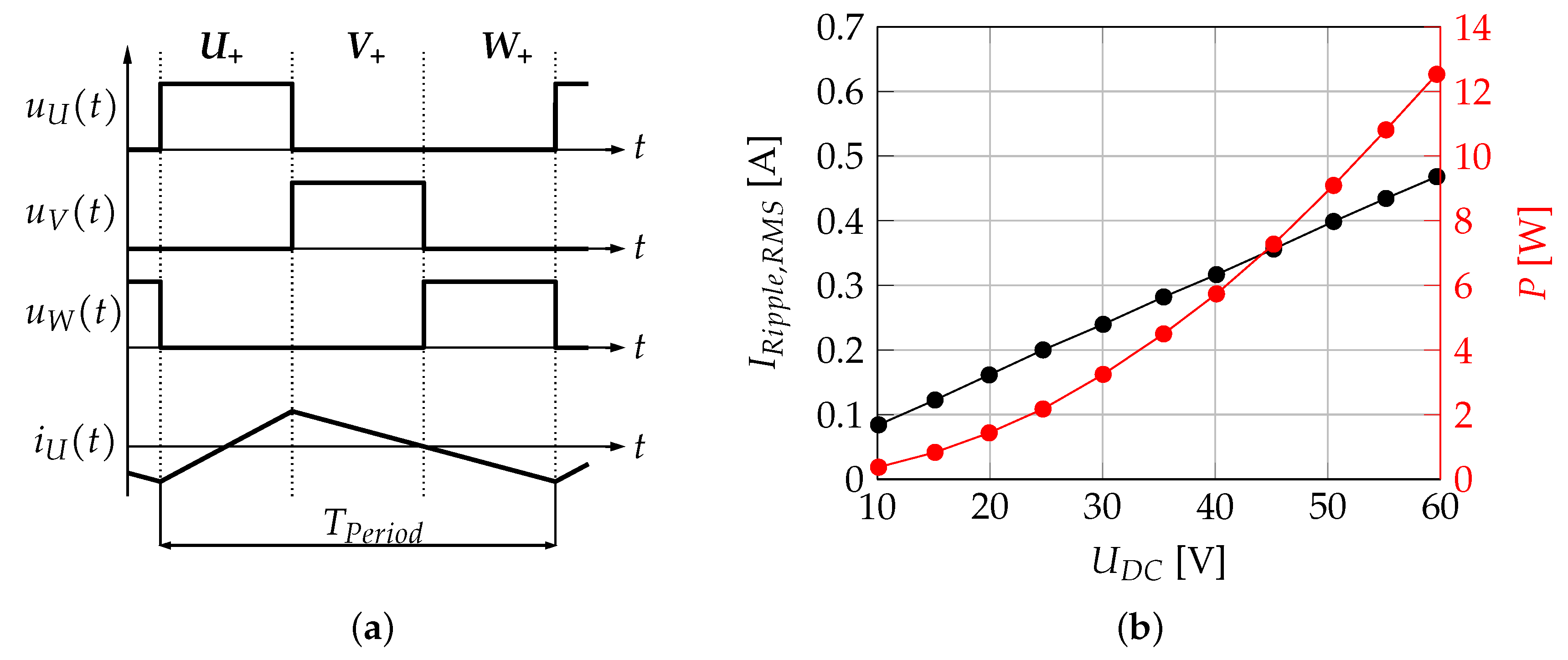
Beside the control current, the current ripple of the coils causes remarkable power losses in the AMB. Hence, major power losses in the prototype occur in the flux leading paths by means of iron losses in the laminated iron sheets. One possible solution for the reduction of the eddy current losses is the use of soft magnetic composites (SMC), which is described in [18]. However, SMC materials have drawbacks like a smaller permeability and mechanical limitations [19]. This work follows an approach, which is independent of the used material. Figure 5a shows the 3-Active SVM pattern with the corresponding power losses (Figure 5b) of the prototype as a function of the DC-link voltage .
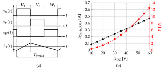
Figure 5.
(a) 3-Active space vector modulation: Each PWM period contains voltage space vectors from each phase (, , ). (b) Power losses of the bearing due to the current ripple as a function of the DC-link voltage (3-Active SVM, ).
For a fixed switching frequency, it is obvious to decrease for achieving small power losses. On the one hand, a high value of causes a high current ripple (Figure 5b), which provides a high magnitude of the differential current slope information. On the other hand, the iron losses are increased and therefore, undesirable power losses occur in the flux leading paths. To keep the power losses in the bearing small, a low level of is aspired. This circumstance gives the motivation to enhance the self-sensing position measurement for dealing with small current slopes. Furthermore, it must be considered that the dynamic of the current controller depends on . The focus of this work lies on the investigation of different space vector modulations to ensure a sufficient current dynamic as well as a high quality of the position measurement. The design of SVM contains degrees of freedom, which can be used for the development of specific pulse patterns with especially high current dynamics or high quality of the position measurement. Taking this one step further, it is possible to use different kinds of SVM during the operation of the AMB. This leads to the variable SVM and enables the combination of the properties of different modulations.
4. Space Vector Modulation
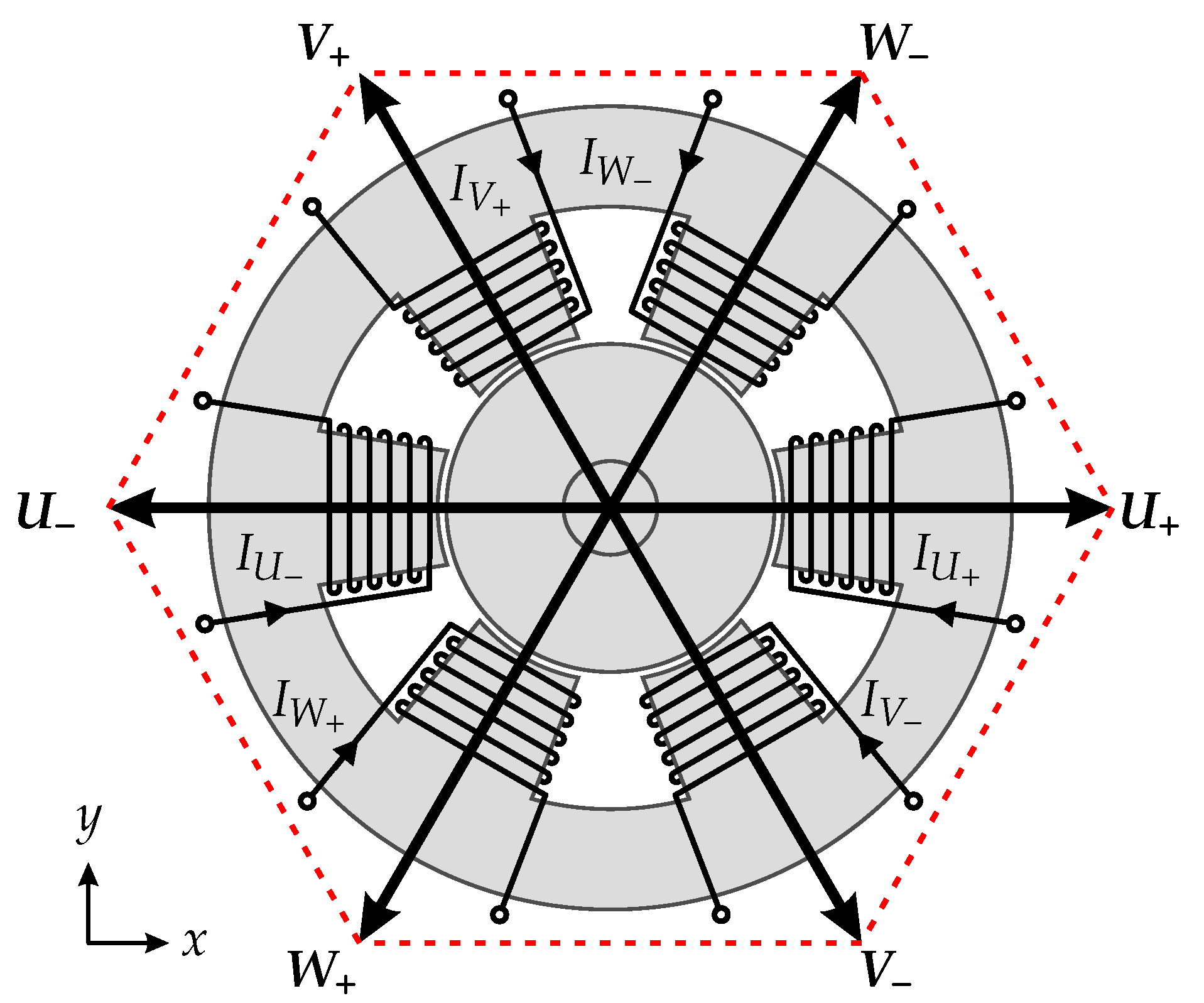
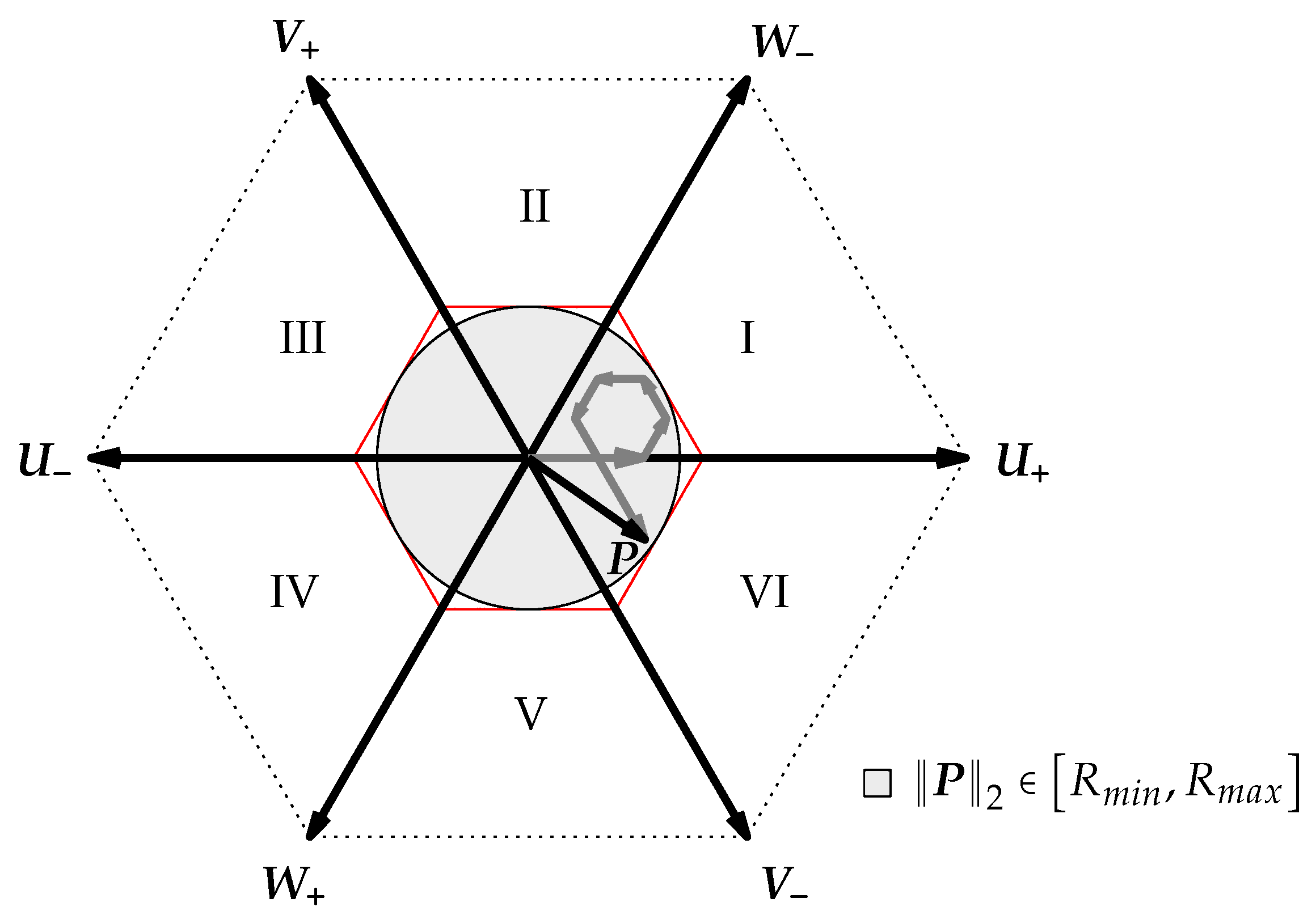
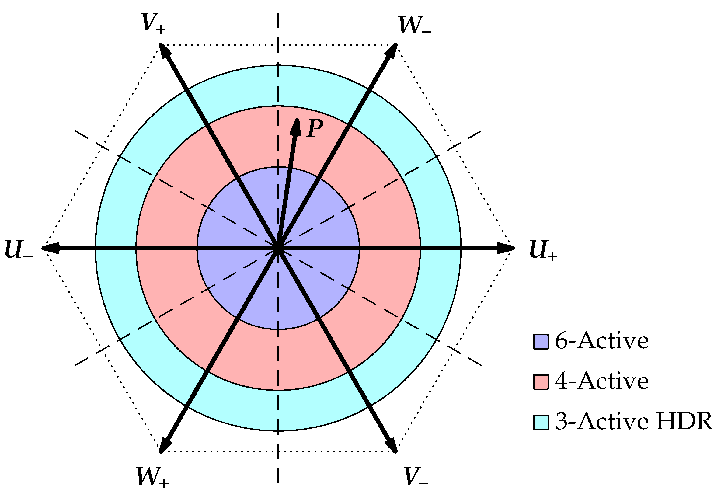
Figure 6 shows the symmetrical arrangement of the magnetic poles of the bearing in the xy-plane. The spatially distributed arrangement of the poles enables the definition of six fundamental voltage space vectors, which are aligned with the magnetic poles of the bearing. The voltage space vectors can be obtained by a conventional power inverter with three half bridges by the switching states shown in Table 1 [20].
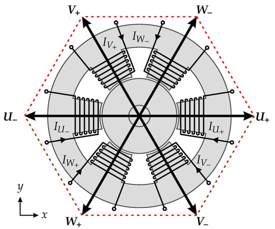
Figure 6.
Cross section of the six pole homopolar radial AMB. The fundamental voltage space vectors , , , , , are aligned with the poles.

Table 1.
Voltage space vector definition of a three-phase inverter.
The fundamental space vectors shape a hexagon, which defines the possible modulation range of the voltage space vectors. Each point in this hexagon can be reached by a linear combination of six fundamental space vectors (, , , , , ) and two zero space vectors (, ). The zero space vector occurs if either all high-side or low-side switches of the three-phase inverter are closed. The calculation between the reference coordinate system (x, y) and the three phase system (U, V, W) is done by the Clarke-transformation [21]. The degree of freedom in the composition of the linear combination of the space vectors is restricted by the following design rules for self-sensing operation.
4.1. Design Rules for SVM
The design criteria of the SVM achieve a good quality of the position measurement and a high current controller bandwidth. Therefore, the design of the SVM underlies certain restrictions to allow a self-sensing operation of the magnetic bearing:
- INFORM method: Theoretically, the current ripple caused by a single voltage pulse contains the whole information of the rotor position. As asymmetries appear in the real system (caused by mechanical, electrical or magnetic deviations), it is beneficial to use the current slope information from independent voltage pulses. Furthermore, the voltage pulses must have a minimal pulse duration , which is given by the settling time of the current slope measurement path (Figure 3b). The duration is defined by the decay of the eddy currents and the settling of the analog filter, which causes a distortion of the differential current slope signal.
- Modulation amplitude: The modulation amplitude defines the maximum length of a desired voltage space vector. High modulation amplitudes of the desired voltage space vector allow a high dynamic of the current control. For a symmetrical (angle independent) operation of the current controller, it is beneficial to limit the modulation amplitude to the in-circle of the possible modulation area. Theoretically, the symmetrical modulation amplitude can achieve a value of for the given AMB system.
- Inverter: Short pulse lengths could cause problems in semiconductor switches. Hence, the specified recovery time of the switches must be considered in the PWM pattern [22]. Furthermore, a proper operation of a potential charge pump of the gate driver must be ensured. Therefore, the pulse pattern has to provide at least one switching action in each phase.
The design procedure of the SVM is based on a representation of the desired voltage space vector , which is specified by the superior current controller. Hence, the desired space vector is given by means of all eight voltage space vectors.
Therefore, the coefficients , , , , , , , define the length of the corresponding space vector. The length of the respective voltage space vector is related to the duration of the voltage pulse in the PWM pattern. The following introduced variants of SVM differ substantially in the number of the active space vectors within one PWM period. In this context, “active” refers to the fundamental space vectors with an amplitude unlike zero. In the following considerations the minimum pulse duration is normalized to the PWM period.
4.2. 6-Active SVM
The 6-Active SVM uses all fundamental space vectors for the formation of . Hence, is built by a linear combination of the adjoining fundamental voltage space vectors. The remaining time of the PWM period is equally distributed to all fundamental voltage space vectors to build a combined zero space vector. The maximum modulation amplitude is obtained, if the length of one active space vector drops under and violates the timing requirements of a differential current slope measurement. Although the admissible modulation area is defined by the solid hexagon in Figure 7, the intended modulation area is limited by the minimum and maximum symmetrical modulation amplitude (, ).
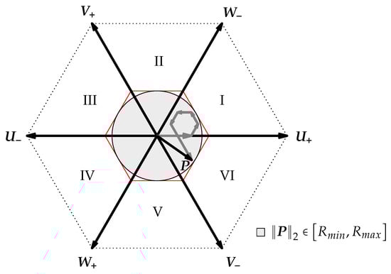
Figure 7.
6-Active SVM: The space vector is formed by six fundamental space vectors ().
The 6-Active SVM allows six independent current slope measurements within a PWM period. For this reason, the 6-Active SVM is well suited for the self-sensing method. However, this kind of modulation has the drawback of a very limited modulation amplitude . The impact of the small value of is caused by the minimal pulse width by means of Equations (3) and (4).
For achieving a higher value of , the number of space vectors is reduced in the following considerations.
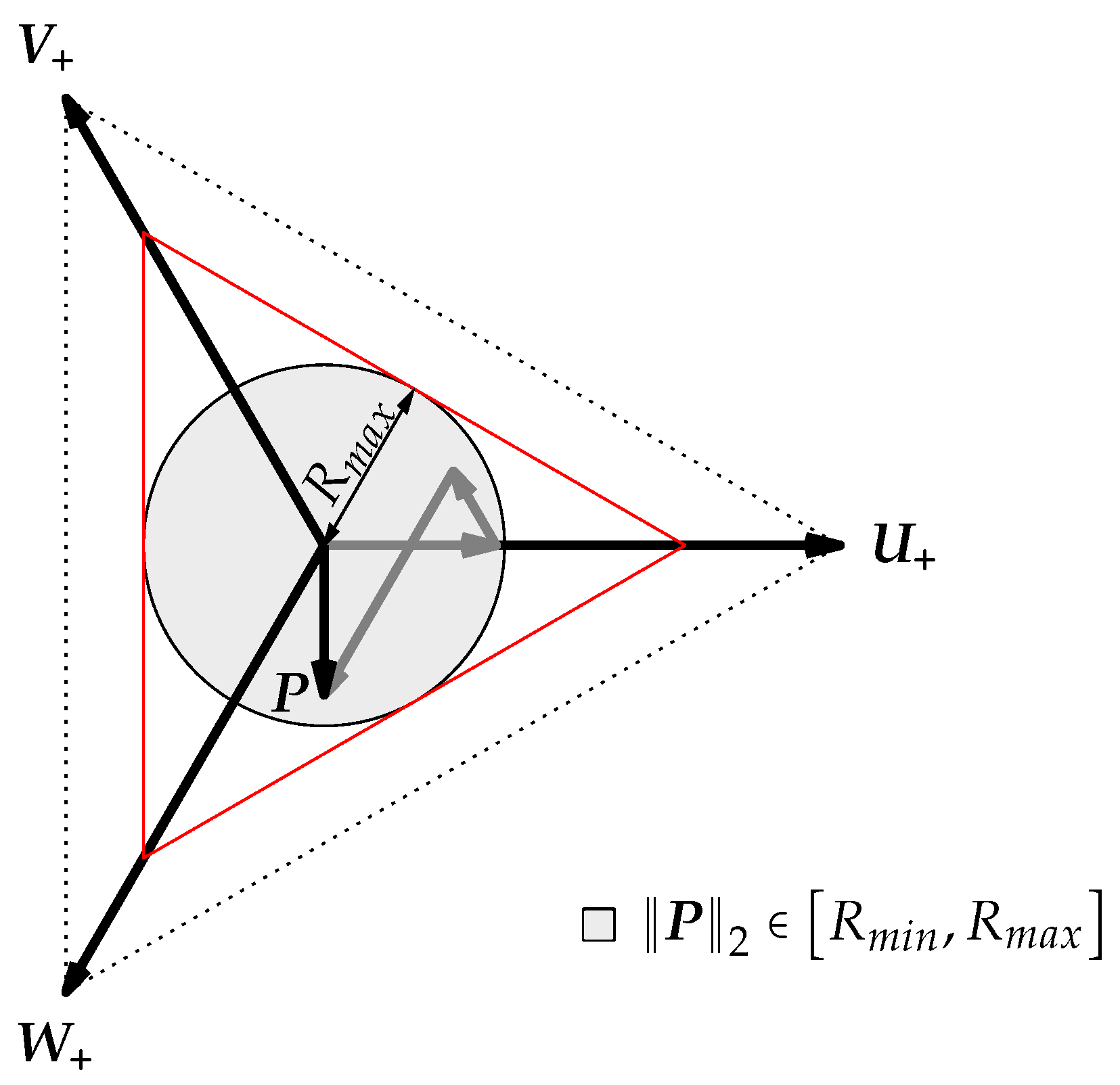
4.3. 3-Active Low Dynamic Range SVM
In contrast to the 6-Active SVM, the 3-Active Low Dynamic Range (LDR) SVM uses either three positive (, , ) or three negative fundamental space vectors (, , ).
Figure 8 shows a 3-Active LDR SVM with a linear combination of , , . The corresponding coefficients from Equation (2) can be calculated by the inner product of and the respective fundamental voltage space vector (Equations (5)–(7)).
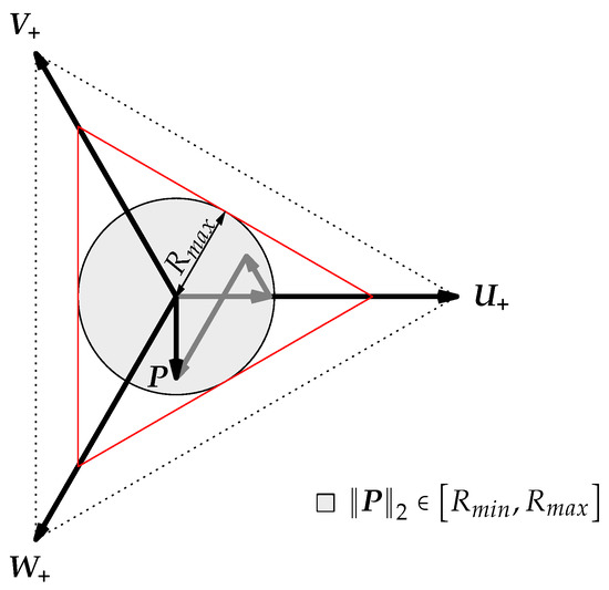
Figure 8.
3-Active LDR SVM: The space vector is formed by the positive fundamental space vectors (, , ). ().
By using only three fundamental space vectors, the maximum modulation amplitude is limited to and causes a smaller drop of
by an increase of than the 6-Active SVM.
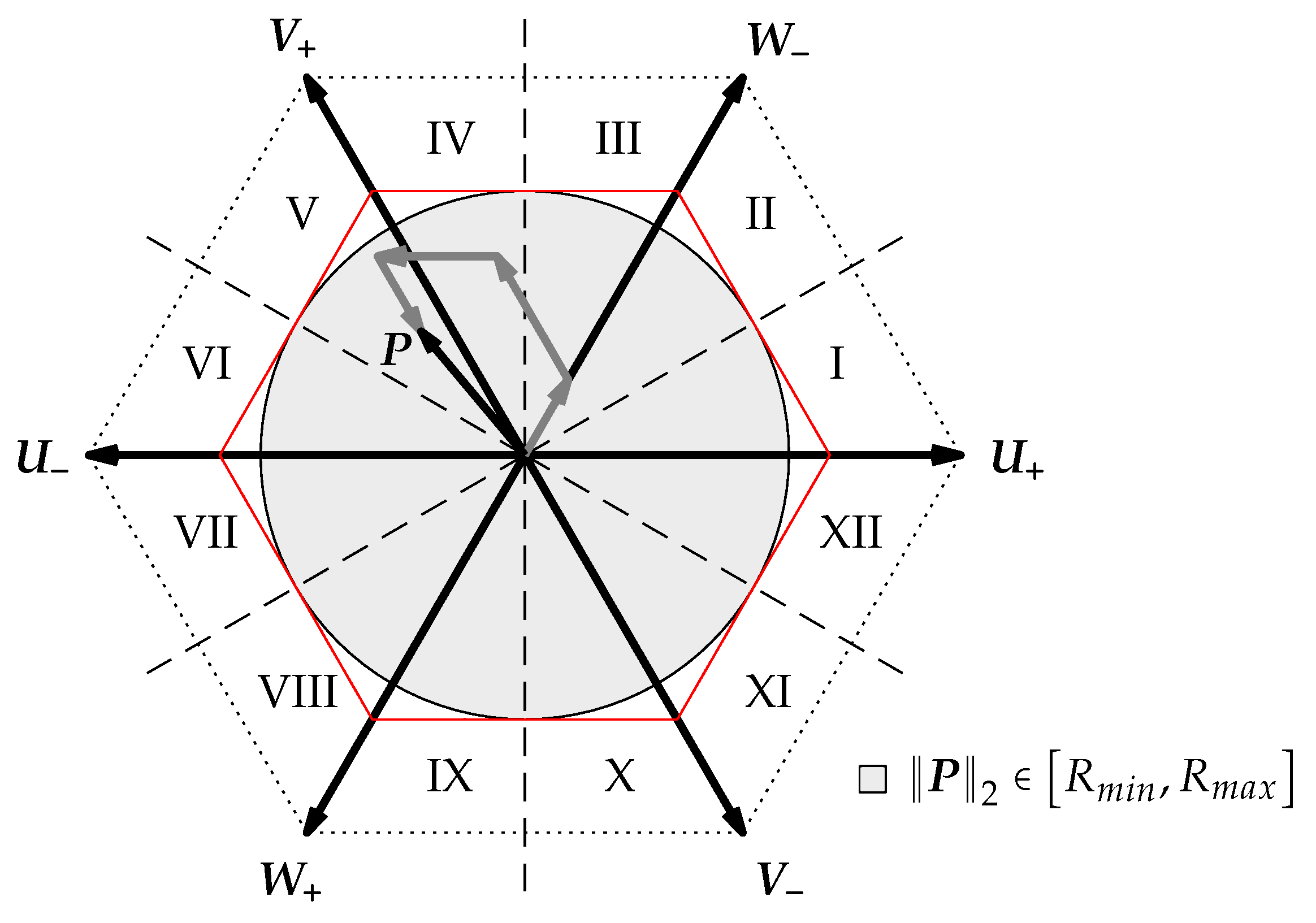
4.4. 4-Active SVM
The 4-Active SVM is based on the 3-Active LDR SVM, but enhances the modulation amplitude by means of an additional fundamental voltage space vector, which is located next to the desired space vector like shown in Figure 9. For an effective implementation, the desired space vector is built by a linear combination of the adjoining fundamental voltage space vectors. The remaining time of the PWM period is distributed equally to the positive (, , ) or negative (, , ) fundamental voltage space vectors.
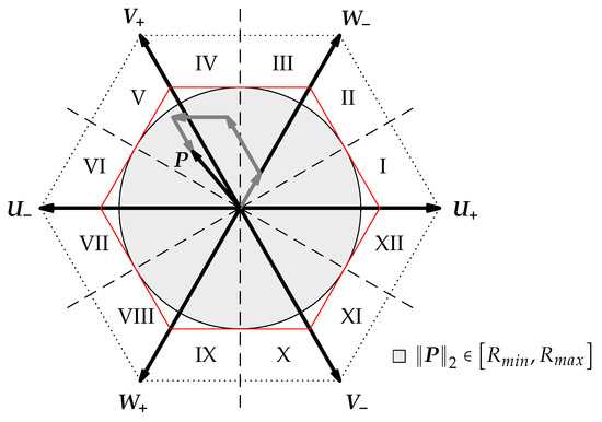
Figure 9.
4-Active SVM: The space vector is formed by the negative (, , ) fundamental space vectors and for an enhancement of the modulation amplitude ().
The limits of the symmetrical modulation amplitude
are obtained if the length of one vector falls below . In contrast to the 3-Active LDR SVM, the maximum modulation amplitude is enhanced by a factor of (Equation (10)).
4.5. 3-Active High Dynamic Range SVM
The 3-Active High Dynamic Range (HDR) SVM is designed for a maximum modulation amplitude using three fundamental space vectors and one of the zero space vectors (, ). The desired space vector is mainly formed by the two adjoining fundamental space vectors (, in Figure 10).
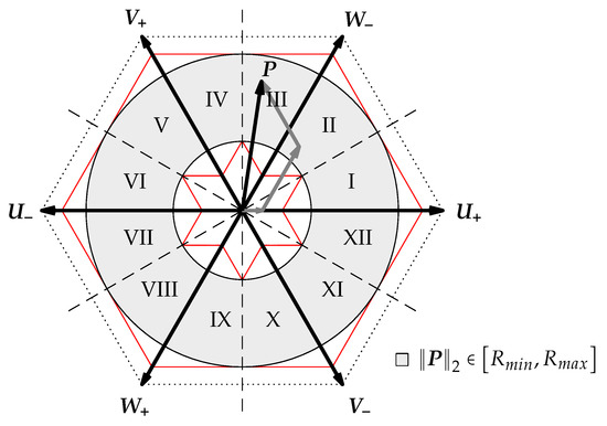
Figure 10.
3-Active HDR SVM: The desired space vector is built with three fundamental space vectors (involving a space vector from each phase) and one zero space vector ().
In order to get a current slope information by a voltage space vector from all space axis, the third fundamental space vector ( in Figure 10) is added with the minimum length . A zero space vector fills the remaining time of the pulse pattern and ensures the required switching action in each phase. Equations (12) and (13) show the possible modulation range
for a symmetrical operation.
4.6. Combination of the SVMs
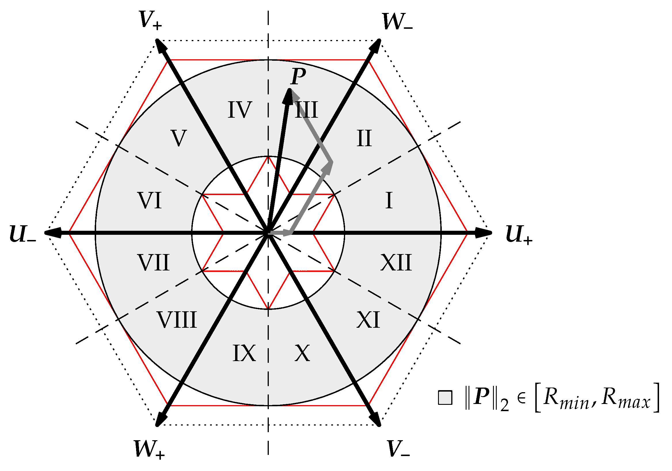
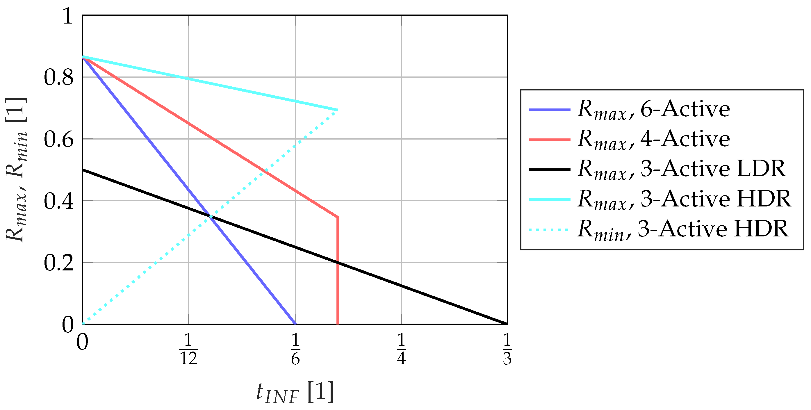
The design of the SVMs shows, that each SVM has individual characteristics concerning the modulation amplitude and the usability for self-sensing operation. For an optimal operation of the bearing, it is possible to combine the properties of different SVMs. Figure 11 shows a comparison of the symmetrical modulation amplitudes as a function of .
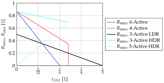
Figure 11.
Comparison of the symmetrical modulation amplitude.
The 3-Active HDR has the property of a lower boundary of the modulation amplitude. It is obvious, that a low value of leads to a high maximum modulation amplitude. The 3-Active LDR can operate up to , which can be advantageous for applications with a high switching frequency. Concerning the performance of the self-sensing operation, each fundamental space vector gives additional information for the rotor position.
Figure 12 shows a combination of multiple SVMs for . The choice of the SVM is determined in a way, that the desired space vector is built by the SVM, which provides the highest number of active space vectors within a PWM period. To avoid nonessential switching between different SVMs, a hysteresis can be defined by means of an overlapping modulation area.
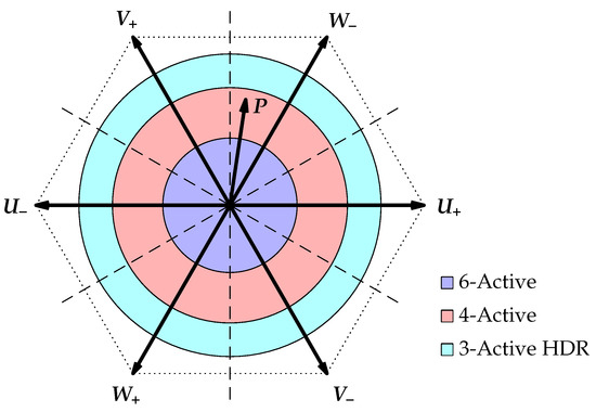
Figure 12.
Combination of different SVMs during operation for achieving a high modulation area and a maximum performance of the self-sensing position measurement ().
4.7. SVM Switchover
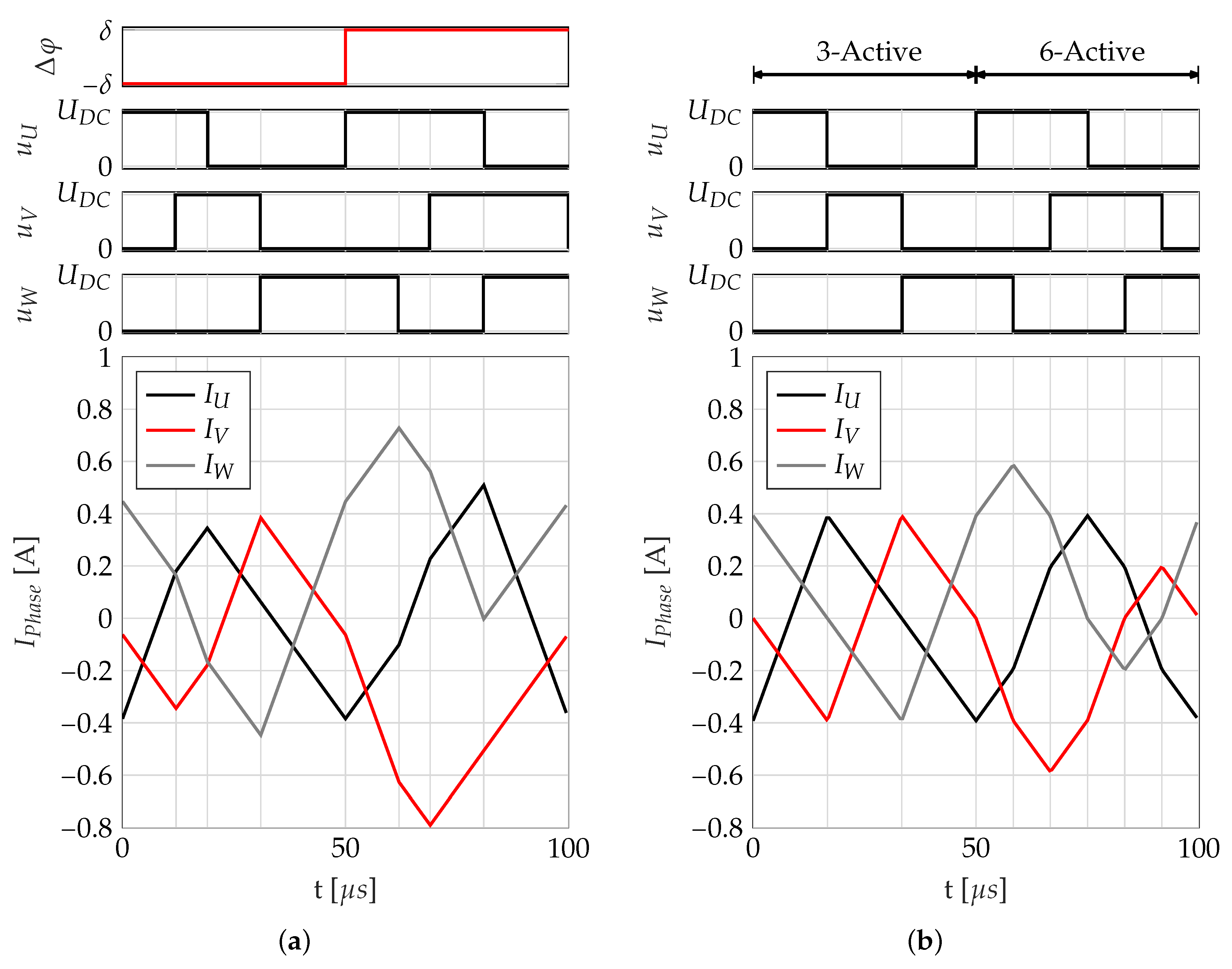
It is possible to make a distinction between two scenarios of SVM switchover. The first scenario is a sector switchover within a SVM. In the 4-Active and 3-Active HDR SVM the fundamental voltage space vectors used depend on the sector of . Thus, the fundamental space vector changes if changes to a new sector of the modulation area. Therefore, a switchover of the sector causes a change in the current ripple profile. Although the steady state of the mean value of the current is not affected by this effect, the phase currents obtain a transient error by a sector switchover. The amplitude of the current error is in the range of the amplitude of the current ripple. Figure 13a shows a simulation of a sector switchover for the 4-Active SVM for a space vector with and . It can be seen that the mean values of the phase currents differ after the sector switchover, which result in a transient deviation that decays over time.
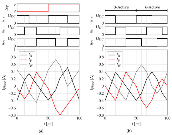
Figure 13.
(a) Transient simulation of a sector switchover within the 4-Active SVM. The voltage space vector has an amplitude of zero but changes in the angle to force a sector switchover. (b) Transient simulation of a switchover between the 3-Active and 6-Active SVM. Both SVMs represent a voltage space vector with zero amplitude ().
The second scenario is given by a switchover between different SVMs. Figure 13b shows a switchover between the 3-Active LDR and the 6-Active SVM for the voltage space vector and . Although both SVM represent a zero space vector, a drift of the mean values of the currents can be observed after the switchover. This effect is caused by the different current waveforms of the SVMs. In many applications, the current ripple is significantly smaller than the control current and the drift due to sector switchover is negligible. However, if the application requires a precise current control beneath the amplitude of the current ripple, a compensation strategy is required. One conceivable solution would be the introduction of a modified PWM cycle to suppress the current drift after a SVM switchover.
5. Measurements
The following measurements compare the behavior of the designed SVMs, regarding power losses, dynamic of the current controller as well as the quality of the self-sensing position measurement. The measurements were performed on the prototype presented in Figure 4 applying the test setup of Figure 14. External eddy current-based position sensors were used as a reference for position measurements.
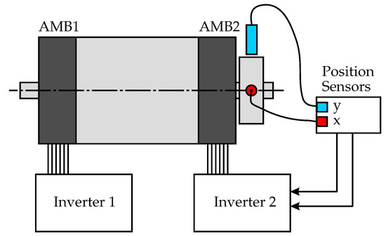
Figure 14.
Symbolic arrangement of the test setup with external position sensors according to Figure 4.
The test setup with two homopolar radial magnetic bearings was controlled by independent three-phase inverters. Basically, a decoupled control of the rotor gives many degrees of freedom for advanced control [23]. However, simple decentralized PIDT1 position controllers provided sufficient performance for the following considerations. Concerning position control, it was assumed that the force on the rotor is proportional to the phase currents. In general, the currents of opposite coils (e.g., , ) are not equal due to different inductances of an eccentrically levitating rotor. Therefore, the implemented force control by means of a static current force characteristic [24] is an approximation, but it does not cause any restrictions for the subsequent measurements.
5.1. Power Losses of the SVM Variants
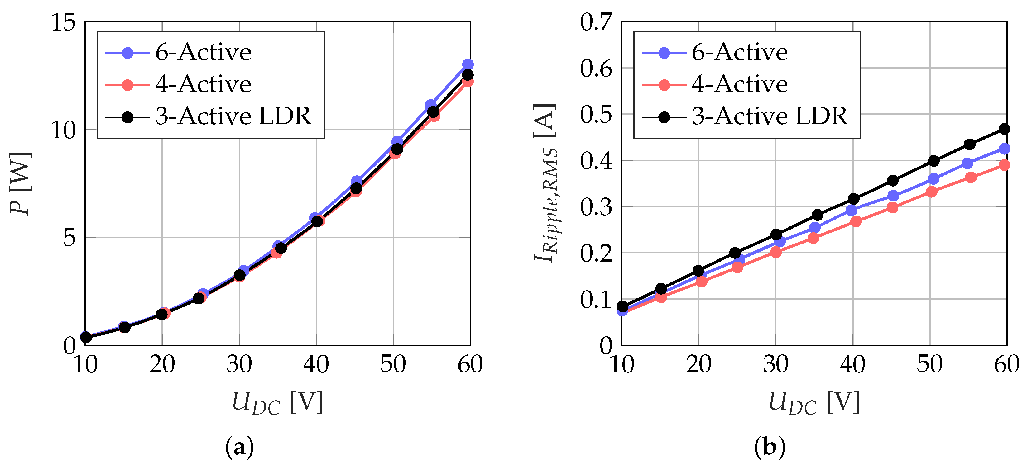
The initial aim was to decrease the power losses in the bearing by a reduction of the DC-link voltage. Figure 15 shows a comparison of the power losses in the bearing for different SVMs at 20 kHz switching frequency. There is no significant difference between the SVMs, which allows an almost power neutral switchover between different SVMs.
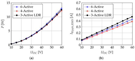
Figure 15.
Comparison of the power losses in the bearing (a) and the current ripple of a phase (b) as a function of the DC-link voltage (, ).
5.2. Dynamic of the Current Controller
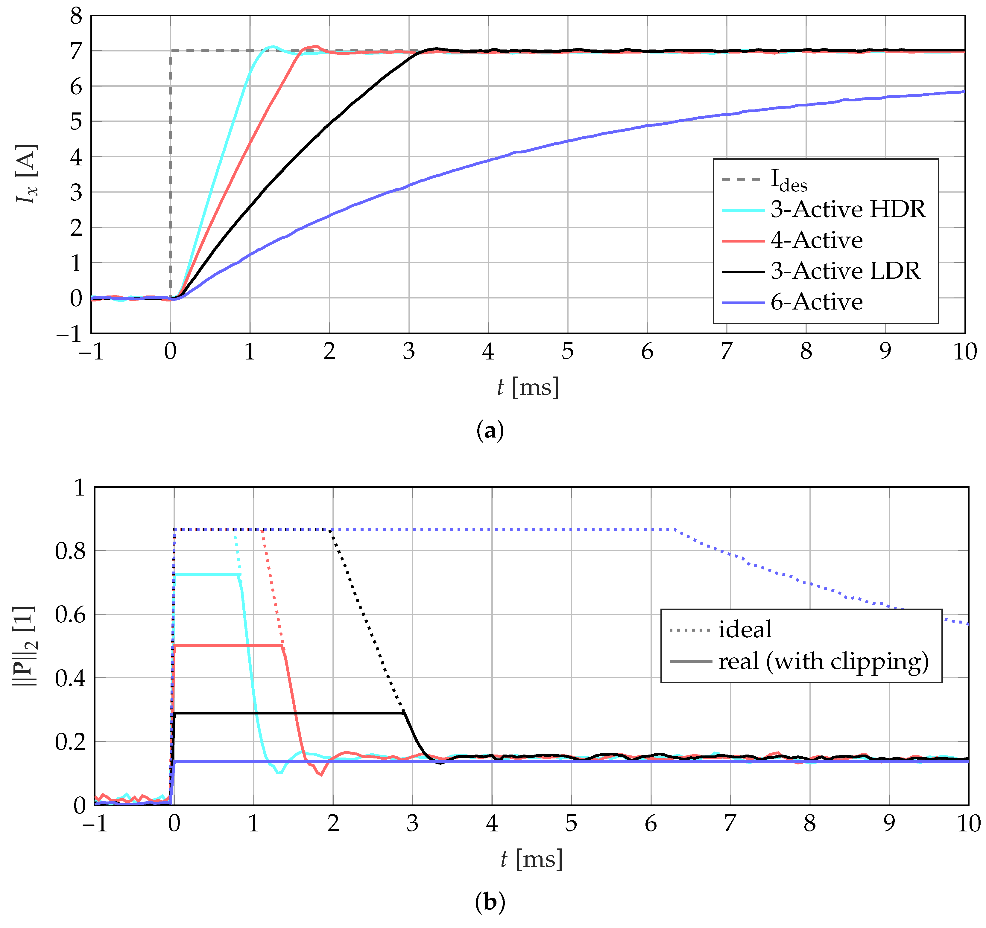
The maximum modulation amplitude of the particular SVM has a significant impact on the dynamic of the current controller. Figure 16a shows a dynamic comparison of the current controller by means of the step response. Due to the fact that the 3-Active HDR SVM is not able to represent a modulation amplitude smaller than (Figure 11), it is combined with the 4-Active SVM to obtain a steady state without oscillation.
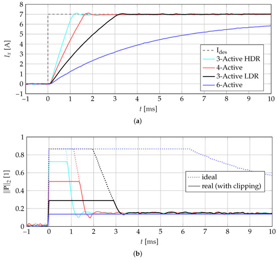
Figure 16.
(a) Step response of the current controller for different SVMs. (b) Corresponding magnitude of the desired voltage space vector (, , ).
Figure 16b indicates the amplitude of the desired voltage space vector , which corresponds to the step response. It can be seen, that the 3-Active HDR SVM has the highest modulation amplitude. Thus, the controller is only saturated for a short period of time at . Concerning Figure 16, the 6-Active SVM is not able to inject the desired current of 7 A to the coil. The reason is the coil resistance and the connector cable. In this case, the 6-Active modulation can only be used for small currents and shows the use case for switching to a SVM with a higher modulation amplitude.
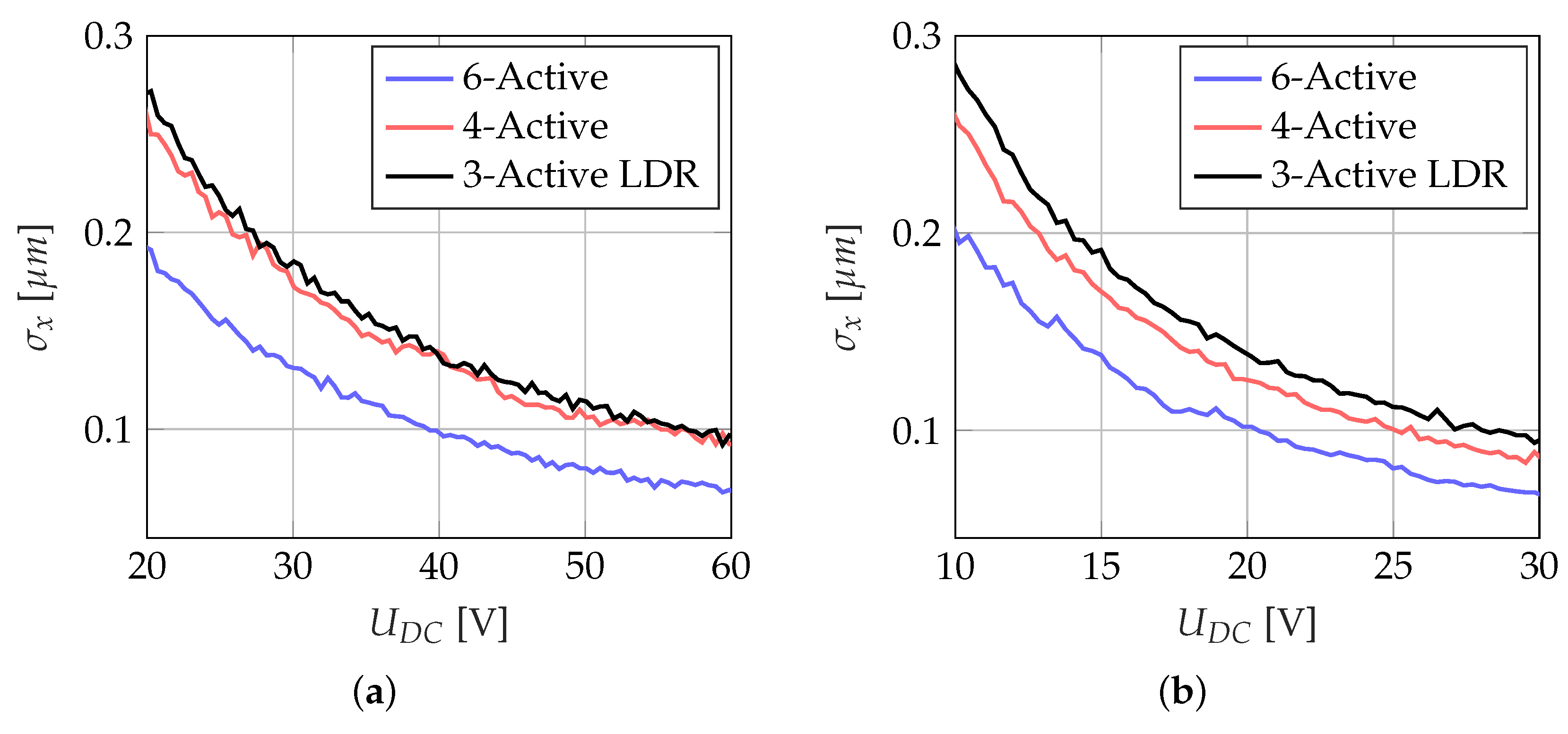
5.3. Noise of the Self-Sensing Method
The noise of the self-sensing method is of great significance for a precise control of the bearing. Figure 17a shows a noise comparison of the different SVMs with in the range of 20 V to 60 V. The 6-Active SVM has the lowest noise level, which is caused by the high number of voltage space vectors within a PWM period. Basically, the noise level increases proportional to . However, it is possible to shift the noise level in a certain range by an adaption of the analog circuit. Therefore, a low noise level can be achieved even at low values of . Thus, Figure 17b shows a similar noise characteristic like Figure 17a at the half DC-link voltage level (e.g., m at 19 V) by means of an adaption of the analog circuit.
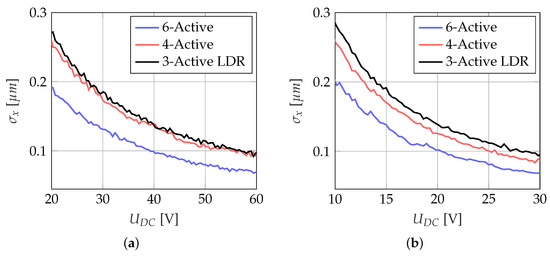
Figure 17.
(a) Noise comparison of the self-sensing position measurement. (b) Reduction of the noise at low levels of by an adaption of the analog circuit (, rotor fixed in the center of the bearing, standard deviation over 3000 samples of the x-position at each setpoint of ).
5.4. Linearity of the Self-Sensing Method
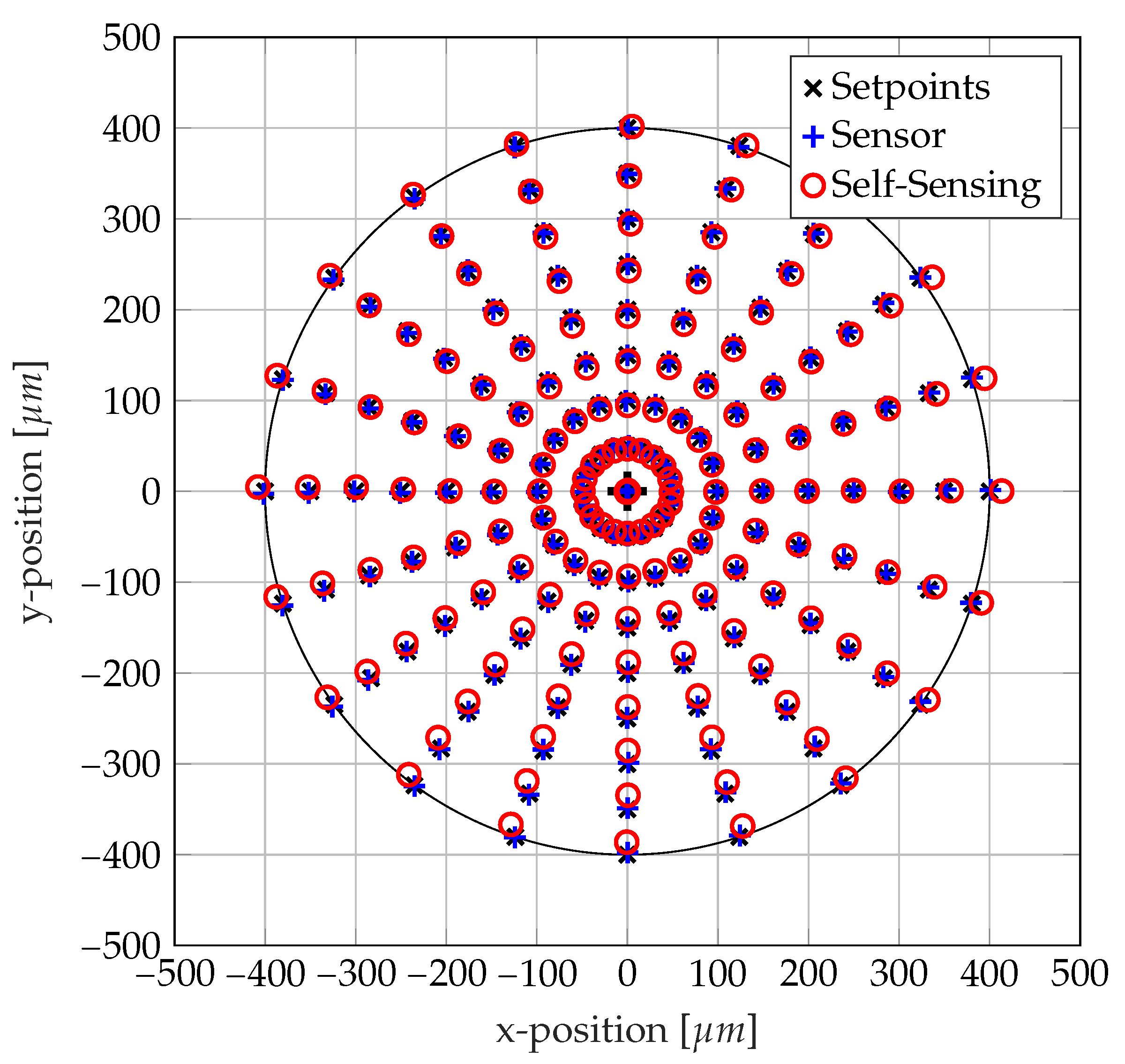
Beside the noise level, the self-sensing method must provide a high linearity for a proper operation of the bearing. The AMB prototype has an air gap of 800 m and the auxiliary bearing allows a radial operational range of 400 m. Figure 18 shows a linearity analysis of the 6-Active SVM with external position sensors for different rotor setpoints.
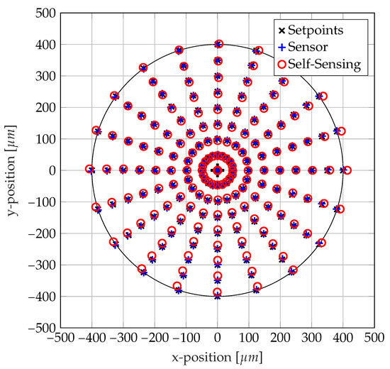
Figure 18.
Linearity analysis with external position sensors for different setpoints of the rotor position (, 6-Active SVM).
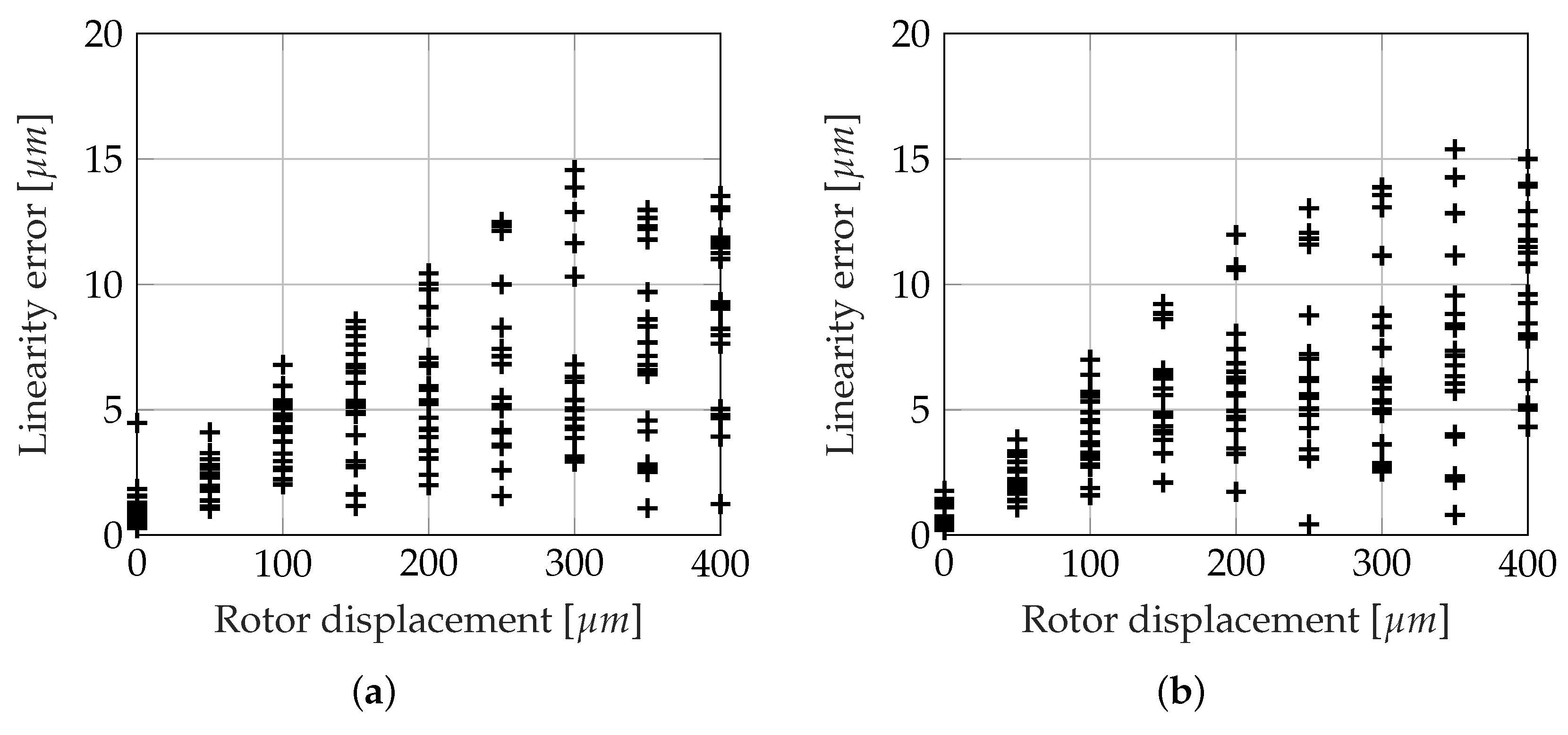
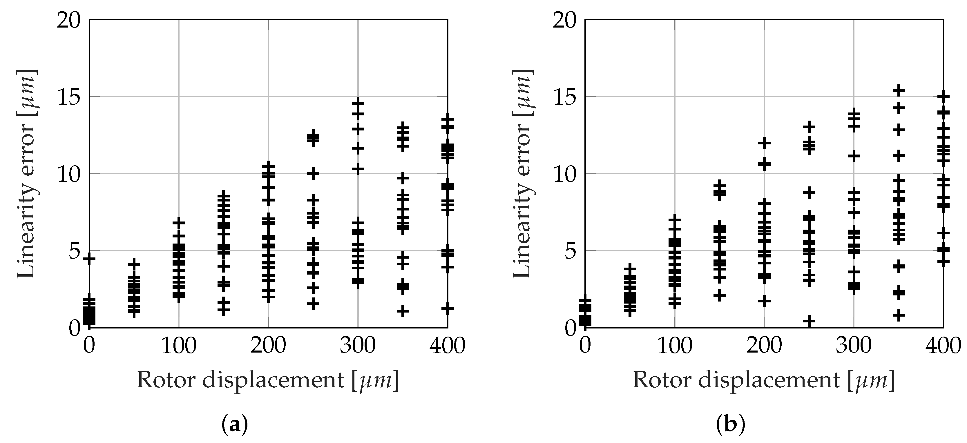
The external sensors measure the rotor position on an aluminum disc, which is mounted close to the magnetic bearing. Due to an axial and angular shift of the sensors with regard to the AMB, the position information of the sensors is transformed in the self-sensing coordinate system. Figure 19 shows the self-sensing linearity error for different rotor positions for a SVM with 3 and 6 active voltage space vectors. It can be seen that the SVMs have a similar distribution of the linearity error with a maximum linearity error of about 16 m.
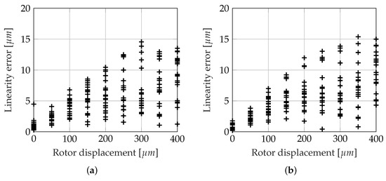
Figure 19.
Analysis of the self-sensing linearity error as a function of the radial rotor displacement for different SVMs: (a) 3-Active LDR, (b) 6-Active.
The linearity of the self-sensing method is important for a proper control of the bearing, especially for robustness considerations of self-sensing magnetic bearings [25,26].
5.5. Small Signal Behavior
Finally, a comparison of the small signal behavior of the self-sensing method was performed. For this purpose, a disturbance is applied to the self-sensing levitating rotor and the sensor signal is shown for comparison (Figure 20). Both signals show a consistent behavior, which manifests a precise self-sensing operation.

Figure 20.
Comparison of the small signal behavior between an external sensor and the self-sensing method. A disturbance is applied at (a) x-position (b) y-position (, 6-Active SVM).
6. Results
The measurements on the prototype demonstrated the characteristics of different space vector modulations concerning self-sensing and current dynamic. The combination of different kinds of modulation allows a high modulation amplitude of voltage space vectors. This feature enables the possibility of a reduction of the DC-link voltage, while still having sufficient dynamic in the current control. Measurements on a prototype showed, that AMB losses due to the current ripple have an approximate square dependence of the DC-link voltage. Therefore, already a small reduction of the DC-link voltage can reduce power losses in the AMB. Furthermore, a measurement of the power losses revealed that the power losses caused by the switching ripple are nearly independent of the used SVM, which enables almost power neutral SVM switchover. The combination of different SVMs leads to a high dynamic of the current controller, which was proven by the step response of the system. An analysis of the switchover characteristics between different SVMs indicated, that a SVM switchover has an impact to the phase currents in the range of the ripple amplitude. This effect may lead to disturbances in the current control and could be suppressed by a compensation cycle in the SVM after a switchover. Regarding the self-sensing position measurement, the experimental results of the prototype showed a low noise level, which varied with the used SVM. A linearity analysis with external sensors showed an overall error of about 16 m for different setpoints in the admissible rotor orbit.
7. Conclusions and Outlook
The focus of this study lied on an improvement of the space vector modulation of a three-phase self-sensing radial magnetic bearing. Different kinds of space vector modulations for self-sensing operation were presented in theory as well as proven in experiments on a prototype of a radial active magnet bearing. The results showed that the dynamic of the current controller and the quality of the self-sensing position control can be adjusted by the choice of the space vector modulation. The self-sensing method showed a high linearity and low noise of the rotor position for low control currents. In a next step, saturation effects of the flux leading paths will be considered regarding nonlinearities of the self-sensing operation to analyze the limitations of the self-sensing control. Further investigations will be performed at various rotational speeds to reveal potential speed-depending effects of the self-sensing control, especially with respect to a robust control of the system.
Author Contributions
Conceptualization, D.W., M.H. (Markus Hutterer), M.S.; methodology, D.W., M.H. (Markus Hutterer); software, D.W.; validation, D.W., M.H. (Markus Hutterer); formal analysis, D.W., M.H. (Markus Hutterer), M.H. (Matthias Hofer); investigation, D.W.; resources, M.S.; writing—original draft preparation, D.W.; writing—review and editing, M.H. (Markus Hutterer), M.H. (Matthias Hofer), M.S.; supervision, M.S.;
Funding
This research received no external funding.
Acknowledgments
This project was supported by Technische Universität Wien in the framework of the Open Access Publishing Program.
Conflicts of Interest
The authors declare no conflict of interest.
Abbreviations
The following abbreviations are used in this manuscript:
| AMB | Active Magnetic Bearing |
| DC | Direct Current |
| HDR | High Dynamic Range |
| LDR | Low Dynamic Range |
| PCB | Printed Circuit Board |
| PM | Permanent Magnet |
| PWM | Pulse Width Modulation |
| SMC | Soft Magnetic Composite |
| SVM | Space Vector Modulation |
References
- Schweitzer, G.; Maslen, E.H. Magnetic Bearings: Theory, Design, and Application to Rotating Machinery; Springer: Berlin, Germany, 2009; pp. 127–145. ISBN 978-3-642-00496-4. [Google Scholar]
- Earnshaw, S. On the Nature of Molecular Forces which Regulate the Constitution of the Lumiferous Ether. Trans. Camb. Philos. Soc. 1842, 7, 97–112. [Google Scholar]
- Sivadasan, K.K. Analysis of Self-Sensing Active Magnetic Bearings Working on Inductance Measurement Principle. IEEE Trans. Magn. 1996, 32, 329–334. [Google Scholar] [CrossRef]
- Maslen, E. Self–sensing for active magnetic bearings: Overview and status. In Proceedings of the 10th International Symposium on Magnetic Bearings (ISMB10), Martigny, Switzerland, 21–23 August 2006. [Google Scholar]
- Schammass, A.; Herzog, R.; Buhler, P.; Bleuler, H. New results for Self-Sensing Active Magnetic Bearings Using Modulation Approach. IEEE Trans. Control. Syst. Technol. 2005, 13, 509–516. [Google Scholar] [CrossRef]
- Hofer, M.; Nenning, T.; Hutterer, M.; Schrödl, M. Current Slope Measurement Strategies for Sensorless Control of a Three Phase Radial Active Magnetic Bearing. In Proceedings of the 22nd International Conference on Magnetic Levitated Systems and Linear Drives (MAGLEV 2014), Rio de Janeiro, Brazil, 28 September–1 October 2014. [Google Scholar]
- Wang, J.; Binder, A. Position estimation for self-sensing magnetic bearings based on the current slope due to the switching amplifier. Eur. Power Electron. Drives (EPE) 2016, 26, 125–141. [Google Scholar] [CrossRef]
- Gruber, W.; Pichler, M.; Rothböck, M.; Amrhein, W. Self-Sensing Active Magnetic Bearing Using 2-Level PWM Current Ripple Demodulation. In Proceedings of the 7th International Conference on Sensing Technology (ICST), Wellington, New Zealand, 3–5 December 2013. [Google Scholar]
- You, S.J.; Ahn, H.J. Position Estimation for Self-Sensing Magnetic Bearings using Artificial Neural Network. In Proceedings of the 16th International Symposium on Magnetic Bearings (ISMB16), Beijing, China, 13–17 August 2018. [Google Scholar]
- Schrödl, M. Sensorless control of permanent-magnet synchronous machines at arbitrary operating points using a modified INFORM flux model. Eur. Trans. Electr. Power ETEP 1993, 3, 277–283. [Google Scholar] [CrossRef]
- Hofer, M.; Hutterer, M.; Nenning, T.; Schrödl, M. Improved Sensorless Control of a Modular Three Phase Radial Active Magnetic Bearing. In Proceedings of the 14th International Symposium on Magnetic Bearings (ISMB14), Linz, Austria, 11–14 August 2014. [Google Scholar]
- Nenning, T.; Hofer, M.; Hutterer, M.; Schrödl, M. Setup with two Self-Sensing Magnetic Bearings using Differential 3-Active INFORM. In Proceedings of the 14th International Symposium on Magnetic Bearings (ISMB14), Linz, Austria, 11–14 August 2014. [Google Scholar]
- Schöb, R.; Redemann, C.; Gempp, T. Radial Active Magnetic Bearing for Operation with a 3-Phase Power Converter. In Proceedings of the ISMST4, Gifu City, Japan, 30 October–1 November 1997; pp. 111–124. [Google Scholar]
- Ahn, H.J.; Jeong, S.N. Driving an AMB system using a 2D space vector modulation of three-leg voltage source converters. J. Mech. Sci. Technol. 2011, 25, 239–246. [Google Scholar] [CrossRef]
- Hofer, M.; Hutterer, M.; Schrödl, M. PCB Integrated Differential Current Slope Measurement for Position-Sensorless Controlled Radial Active Magnetic Bearings. In Proceedings of the 15th International Symposium on Magnetic Bearings (ISMB15), Kitakyushu, Japan, 3–6 August 2016. [Google Scholar]
- Hofer, M.; Wimmer, D.; Schrödl, M. Analysis of a Current Biased Eight-Pole Radial Active Magnetic Bearing Regarding Self-Sensing. In Proceedings of the 16th International Symposium on Magnetic Bearings (ISMB16), Beijing, China, 13–17 August 2018. [Google Scholar]
- Herzog, R.; Vullioud, S.; Amstad, R.; Galdo, G.; Muellhaupt, P.; Longchamp, R. Self-Sensing of Non-Laminated Axial Magnetic Bearings: Modelling and Validation. J. Syst. Des. Dyn. 2009, 3, 443–452. [Google Scholar] [CrossRef]
- Hofer, M.; Hutterer, M.; Schrödl, M. Application of Soft Magnetic Composites (SMCs) in Position-Sensorless Controlled Radial Active Magnetic Bearings. In Proceedings of the 15th International Symposium on Magnetic Bearings (ISMB15), Kitakyushu, Japan, 3–6 August 2016. [Google Scholar]
- Gua, Y.; Zhu, J.G. Application of Soft Magnetic Composite Materials in Electrical Machines. Aust. J. Electr. Electron. Eng. 2006, 3, 37–46. [Google Scholar] [CrossRef]
- Van der Broeck, H.W.; Skudelny, H.-C.; Stanke, G.V. Analysis and Realization of a Pulsewidth Modulator Based on Voltage Space Vectors. IEEE Trans. Ind. Appl. 1988, 24, 142–150. [Google Scholar] [CrossRef]
- Chattopadhyay, S.; Mitra, M.; Sengupta, S. Electric Power Quality; Springer: Berlin, Germany, 2011; pp. 89–96. ISBN 978-94-007-0634-7. [Google Scholar]
- Quang, N.P.; Dittrich, J.A. Vector Control of Three-Phase AC Machines: System Development in Practice; Springer: Berlin, Germany, 2015; pp. 17–59. ISBN 978-3-662-46915-6. [Google Scholar]
- Hutterer, M.; Schrödl, M. Control of Active Magnetic Bearings in Turbomolecular Pumps for Rotors with Low Resonance Frequencies of the Blade Wheel. Lubricants 2017, 5, 26. [Google Scholar] [CrossRef]
- Nerg, J.; Pöllänen, R.; Pyrhönen, J. Modelling the Force versus Current Characteristics, Linearized Parameters and Dynamic Inductance of Radial Active Magnetic Bearings Using Different Numerical Calculation Methods. WSEAS Trans. Circuits Syst. 2005, 4, 551–559. [Google Scholar]
- Maslen, E.; Montie, D.; Iwasaki, T. Robustness Of Self Sensing Magnetic Bearings Using Amplifier Switching Ripple. In Proceedings of the 9th International Symposium on Magnetic Bearings (ISMB9), Lexington, KY, USA, 3–6 August 2004. [Google Scholar]
- Hutterer, M.; Hofer, M.; Schrödl, M. New Results on the Robustness of Selfsensing Magnetic Bearings. In Proceedings of the 15th International Symposium on Magnetic Bearings (ISMB15), Kitakyushu, Japan, 3–6 August 2016. [Google Scholar]

© 2019 by the authors. Licensee MDPI, Basel, Switzerland. This article is an open access article distributed under the terms and conditions of the Creative Commons Attribution (CC BY) license (http://creativecommons.org/licenses/by/4.0/).