Abstract
This paper shows the possibility of the measurement of a temperature field generated by heated fluid from a synthetic jet (SJ) actuator. Digital holographic interferometry (DHI) was the main measuring method used for the experiments. A single-projection DHI was used for the visualization of the temperature field as an average temperature along the optical axis. The DHI results are compared with data obtained from constant current anemometry (CCA) experiments for the validation of the method. Principle of 3D temperature distribution using a tomographic approach is also described in this paper. A single SJ actuator, multiple continual nozzle, and the SJ actuator with two output orifices are used as a testing device for the presented experiments. The experimental configuration can measure high-frequency synthetic jets with the use of a single slow-frame-rate camera. Due to the periodic character of the SJ flow, synchronization between the digital camera, and the external trigger driving the phenomenon is performed. This approach can also distinguish between periodic and random parts of the flow.
1. Introduction
Heat transfer measurement is a complex discipline that is extended into many scientific and industrial sectors. The problem is solved in many applications, as are, e.g., heat exchangers [1,2], turbines [3,4,5,6], sustainable energy [7,8,9], chemical processes [10,11,12], or (micro) electronics cooling [13,14,15,16]. Especially in micro-electronic coolers, the flow regime is usually laminar, with a very small Reynolds numbers (in the order of 102). Therefore, transfer processes such as mixing and cooling are typically based on gradient diffusion [17,18,19,20]. The heat transfer processes can be enhanced with the actuation of the laminar flow, creating a so-called “quasi-turbulent” flow character [19]. In these cases, a synthetic jet actuator [17,18,19,20,21] or other vortex generators [22,23,24] can be used effectively.
As is known, a synthetic jet (SJ) is generated by the periodic motion of an actuator oscillating diaphragm (for a schematic view, please see Figure 1a). An SJ is synthesized by interactions within a train of vortex rings or counter-rotating vortex pairs in axis-symmetric or two-dimensional geometry; see [25,26]. Vortex rings that are formed at the lip of the orifice (see Figure 1b) move from the actuator orifice with velocity, which must be high enough to prevent their interaction with the suction force in the orifice. These vortexes dissipate, and the SJ has the characteristics of a conventional steady jet downstream from the orifice (approx. 8D [26]). One of the main advantages of an SJ is that the time-mean mass flux of the oscillatory flow in the orifice is zero; therefore, the requirement of a blower and piping for the fluid inlet is eliminated. Even though the time-mean mass flux in the orifice is zero, the momentum of the resultant SJ at a specific distance from the lip is non-zero [25,26,27,28]. To reach the highest efficiency of an SJ, the actuator should work at the resonance frequency [17,18,26,28]. The frequency response of a double-orifice SJ actuator is investigated in [29].
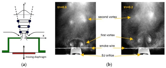
Figure 1.
(a) Schematic view of the synthetic jet, (b) SJ vortex visualization by smoke wire (experiment by Dancova in [36]).
For the SJ investigation, a lot of experimental methods can be used, and it can be divided into two main groups—contact and non-contact. In the case of the contact method, the sensor is placed inside the measured medium, and it affects not only the measured results, but also the phenomenon itself. An example of the contact method for the SJ temperature field measurement is constant current anemometry, based on a change of electrical resistance [30,31]. To prevent the affection from the placed probe, the non-contact method is suitable for use. Non-contact methods that are used to measure temperature distributions can be e.g., the following: the Schlieren method [32], absorption spectroscopy [33], Rayleigh and Raman scattering [34], and methods based on thermal radiation [35].
A very useful non-contact optical technique is holographic interferometry (HI) based on the holography principles discovered by Gabor in 1948, as a lenseless process for image formation by reconstructed wavefronts [37]. The breakthrough of holography was initiated by the development of the laser, providing a powerful source of coherent light at the beginning of the 1960s. The drawback of Gabor’s inline arrangement was addressed by the off-axis technique [38]. Besides the impressive display of three-dimensional scenes exhibiting effects such as depth and parallax, holography has found many applications in the field of synthetic holograms [39,40,41] or holographic data storage [42]. Another application of holography is a measurement technique called holographic interferometry [43,44]. Its early applications ranged from the first measurement of vibration modes [43,44] over deformation measurement [45,46] and contour measurement [47,48], to the determination of refractive index changes [49,50,51]. The wet chemical processing of the holographic recording media with inherent drawbacks has been overcome by capturing a hologram digitally, and even more rapidly after the wide spread discovery of modern cameras by using CCD (charge-coupled device) or CMOS (complementary metal–oxide–semiconductor) [52,53,54]. The most significant impact of digital holography exhibits in digital holographic interferometry (DHI) [55,56,57] and digital holographic microscopy (DHM) [58,59,60,61]. By applying the tomographic approach, DHI enables the measurement of the investigated phenomena not only in 2D [62,63] but also in 3D [64].
DHI as a full-field and very sensitive method for measuring refractive index variations within the measured volume is a very powerful technique for the visualization and measurement of SJ flow. The results of the measurements can be used for the optimization and characterization of the mechatronic parts of the actuator.
This paper provides a comprehensive overview of several experimentally validated DHI approaches and their limits, as they are used for different types of actuators.
2. Digital Holographic Interferometry
Digital holographic interferometry (DHI) is a non-contact, non-invasive, and highly accurate experimental method for measuring quantities that affect the phases of a light wave passing through or reflected from the measured object. It can be used, for example, in the field of mechanical stress and deformation analysis, vibration analysis, or to measure the distribution of the refractive index in a transparent environment, as in case of measuring the temperature field distribution in fluids. This method records the intensity of the interference field as a result of the superposition of the object Uo, and the reference Ur wave (digital hologram). Numerical reconstruction following the record is based on the solution of the free space propagation of an optical wave, and it retrieves the complex field (intensity and phase) of the recorded object wave [54,56,57] from the digital hologram.
In the experiment, at least two holograms hi have to be recorded, where index i = 1 or 2 corresponds to the initial (reference) or state of the object after a change. Holograms are recorded on a digital sensor (CMOS or CCD camera), from which complex waveforms Ui are reconstructed as [54,56,57]:
where , is the wavelength of a light (laser), d is the distance of the object from the digital camera, is the complex amplitude of the reference wave, is the inverse Fourier transformation. The symbols and stand for the coordinates in a hologram and an image plane, respectively. The solution of Equation (1) is a numerical representation of a complex optical field.
The intensity and phase distributions of the reconstructed wave can be calculated as:
The value of the interference phase modulo 2π (see Equation (3)), which is influenced by the temperature change in the working fluid, can be determined as (see [56]):
The relationship between the interference phase and the change of the refractive index in the measured volume is given by the relation:
where denotes the change of refractive index in the measured fluid.
Temperature Field Measurements
Equation (5) defines the relationship between the light phase change of the transmitting wave and the refractive index. The solution of the integral (5) depends on the type of the refractive index distribution temperature field, respectively. The simplest is a two-dimensional (2D) temperature field (e.g., temperature boundary layer measurements). A constant temperature is assumed in the direction of the optical axis. The integral in Equation (5) is simplified to:
where is the differential length of the light rays in the measured environment.
Another type of temperature field is a rotationally symmetric field, such as nozzles or flame. The solution of Equation (5) leads to an inverse Abel transformation [56]. To measure general (unsymmetrical) temperature fields, a tomographic approach based on the multi-directional measurement of several different projections has to be applied [64].
However, refractive index change distribution is not a main concern. The temperature T and the refractive index are related by using the Gladston–Dale and ideal gas equations, as [65]:
where is the Gladston–Dale constant, is the air pressure, and is the universal gas constant (8.3143 J·mol−1·K−1). Putting K = 2.26 × 10⁻⁴ m3·kg−1, R = 8.314 J·mol−1·K−1, p = 101.3 kPa, and T = 297 K into Equation (7) yields .
3. Experimental Setup
For the DHI experiments, a Twyman–Green interferometer with double sensitivity was used. The principle and schematic arrangement of the temperature field experiment is shown in Figure 2. A single-frequency Nd:YAG laser (line width < 1.5 MHz i.e., coherence length > 200 m) works with a wavelength of 532 nm and a power of 150 mW. The laser beam is split into two beams by a beam splitter BS1 (beam splitter); the first beam is a reference wave, and the second one is the object wave. Both beams are spatially filtered (SF) and collimated (CO). As the object beam passes through the measured area twice (the second pass when the beam is reflected from the mirror M3), the measurement has double sensitivity. The reference and object waves are recombined by another beam splitter BS2, and the resulting interference pattern (digital hologram) is recorded with a 5 Mpx AVT Stingray-F 504 digital camera. The images are transferred to the computer via the Fire Wire B interface, allowing for a 6.5 FPS frame rate. The entire experiment was placed onto a vibration-isolated optical table.
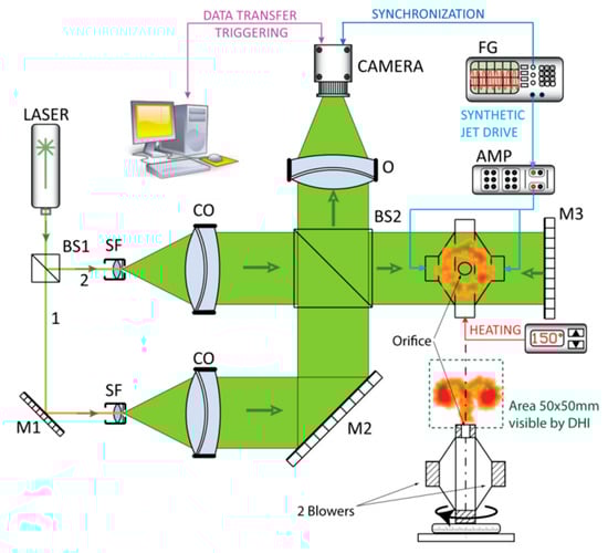
Figure 2.
Schematic view of the experiment using a Twyman–Green interferometer with double sensitivity [66]. BS—beam splitter, SF—spatial filter, CO—collimation objective, O—objective, M—mirror, FG—function generator, AMP—amplifier.
To demonstrate the reliability of the method, a steady temperature field of convective flow of fluid moving up from a system of three orifices was first measured. Secondly, the temperature field under investigation was stimulated by the synthetic jet of fluid.
As the synthetic jet is a non-symmetric (for this prediction, the SJ actuator configuration in Figure 3b is supposed) periodic non-stationary phenomenon, DHI experiments of SJ temperature fields were performed by using a tomographic approach.
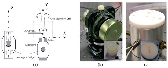
Figure 3.
Experimental arrangement of the SJ actuators for DHI measurement: (a) Schematic view of the actuator, which consists of a heating cartridge, a pair of loudspeakers, and an orifice (the loudspeakers are not mentioned, and are shown in picture 3(a)) [67], (b) the pair of loudspeakers, and the detailed view of the two output orifices for the second actuator, (c) a detailed view of the steady (continual) nozzle with three output orifices.
To investigate the SJ temperature field, two types of SJ actuators were used. Both of these types consisted of a sealed cavity, an upwardly oriented outlet orifice, and two loudspeakers (ARN-100-10/4) (DD = 94 mm) working in phase, which are used as moving diaphragms. The loudspeakers were fed with 1.5 W power. In-phase working loudspeakers have the same direction of movement, which ensures that the fluid is sucked into the SJ actuator during the first part of the period, and extruded in the second part of the period. The whole process is cyclically repeated. The first type of SJ actuator had a single orifice with a diameter D = 5 mm; the second type had two orifices with a diameter D = 2 mm each; the spacing between axis of these orifices was 7 mm. The working frequencies of the first and of the second actuator were 15 Hz and 8 Hz, respectively. A schematic view of both SJ is visible in Figure 3. Figure 3b shows the details of the output orifice of the second actuator SJ. For the tomographic approach validation (described in Section 4.2), the continual nozzle with three output orifices (with a diameter of 3 mm each) was used (Figure 3c). The distance of the adjacent nozzle axes was 12 mm.
For the purposes of the experiment, it was necessary to heat the exhausted air from the SJ actuators and the continual nozzle, respectively. Heating was provided with a cartridge heater OMEGALUX CIR-10,301/240 V, which was inserted into the actuator cavity (Figure 3a). The heater was equipped with a K-type thermocouple, which was connected to a PID (proportional–integral–derivative) controller to control the temperature setting up to 200 °C. In this case, the PID controller enabled the heater temperature setting to be less than 0.2 K. However, due to a low value of the heat transfer coefficient from the cartridge to the air in the cavity, the temperature of the measured airflow was much lower. In order to avoid convection, which causes background noise in the temperature measurement, the beginning of the measurement was delayed until the system was in temperature balance.
The aim of the measurement was to measure the volumetric temperature distribution. As a consequence, the flow had to be recorded from different projection angles, due to the tomographical approach. The simultaneous measurement of all projections is complicated, and many digital cameras are needed. Still, the resolution of tomographic back-projection depends on the number of projections, and it is practically impossible to employ more than a few cameras.
A steady flow is assumed to be constant in time. Therefore the system of orifices was mounted onto a remote-controlled rotary stand that enabled 360° rotation. After recording the reference hologram, the actuator was rotated over a range of 0°–178°, with a step of 2°. A measurement was performed after each turn. Then, a 3D temperature field was obtained by using the tomographical reconstruction method.
The flow of SJs consists of three main components: mean temperature, periodic, and random parts. Assuming perfect periodical and coherent behavior of the SJs, the periodic part of the flow is supposed to be constant for the corresponding relative time within the period of the SJ. Such an assumption allows for the measurement of the periodic part of SJ at certain relative times, at different time instants. The measurement is then identical to aforementioned steady flow measurement. The actuator was mounted onto a remote controlled rotary stand, and as the stand rotates, holograms at different projections are captured.
System Synchronization
In the case of periodic SJ measurement, it is necessary to synchronize the SJ actuator with the measuring system, respective to the external trigger of the camera, in order to capture the SJ exactly at a defined relative time. Considering the period of the SJ τ, and a relative time t’ = t/τ within one period, synchronization enables the phase maps to be captured at the well-defined relative time instances, at different periods of the signal t = t’ + M τ, where M stands for an integer. Assuming the coherence of the phenomenon the phase field, is supposed to be constant as M increases. This synchronization principle is shown in Figure 4a. The synchronization of the camera with a measured phenomenon brings three advantages. On the one hand, it is the possibility of measuring the entire period with a camera that has a significantly longer frame time. In this particular example, the SJ actuator operates at a frequency of 15 Hz (the period is 67 ms) and 8 Hz (125 ms), respectively. The 5 Mpx camera used was relatively slow; its maximum frame rate at this resolution was about 6 FPS (167 ms). Therefore, at least 300 FPS at a frequency of 15 Hz is required (i.e., 20 samples per period), or 37 samples per period, at a frequency of 8 Hz. Assuming the similarity of the vortexes exhausted from the SJ actuator orifice in every cycle, it is possible to synchronize the trigger of the individual frames on the camera at a particular chosen phase of the SJ period.
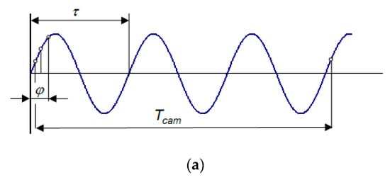
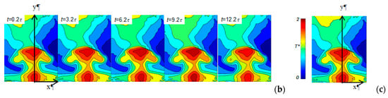
Figure 4.
(a) Due to the synchronization of the camera trigger and the phenomenon, periodic development of SJ with period τ can be captured with a digital camera having a frame period of TCAM at any relative time within the SJ period [67], (b) 2D temperature fields of SJs measured at the same relative time at different periods (M) of the phenomenon. The similarity of the maps proves the coherence of the phenomenon (c); averaged SJ temperature fields from different periods of the phenomenon, see (b).
Another advantage of synchronization is the improvement of the signal-to-noise ratio, and revealing the random flow fluctuations. Instantaneous temperature distribution can be described by its mean value, periodic component, and fluctuating component. The aim of SJ research is primarily focused to the periodic component. By synchronization, many measurements corresponding to the same phase can be obtained; see Figure 4b. An averaging of measurements from different periods at the same phase of fluid flow from the SJ nozzle emphasizes the periodic component of the signal, while the influence of the random component is eliminated. Consequently, the ratio of the periodic and random signal components can be used as a measure, in order to optimize the actuator parameters.
Last but not least, the synchronization of the camera external trigger with the driver of the SJs enables the three-dimensional temperature field distribution of very fast phenomena to be measured with the use of only one digital camera. The “freeze” of the phenomenon (measuring the SJ at a well-defined relative time at different periods of the phenomenon) allows for the SJ periodic component to be measured at different projections that are necessary for the reconstruction of the 3D temperature field.
4. Results
4.1. Validation of Camera Synchronization and 2D Digital Holographic Interferometry
2D DHI is used for a case of the SJ actuator with one output orifice operating at 15 Hz. The left sides of Figure 5 show the development of temperature fields measured with DHI. In this figure, a non-dimensional temperature T* is defined as T* = (T − Ta)/(T0 − Ta), where T is the temperature of the liquid exhausted from the orifice, Ta is the ambient temperature, and T0 is the average temperature in the SJ actuator.
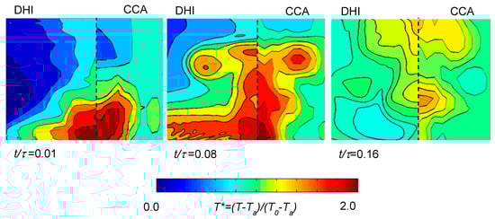
Figure 5.
Temperature field of heated SJ over different t/τ. It has to be noted that the CCA is a point measurement, and that the probe was traversed in the plane x–y, i.e., z = 0, with a step of 1 mm. On the other hand, DHI allows for profile measurements in one moment, and profiles are obtained as mean values along the z-axis.
The figures correspond to different phases during the t/τ cycle, and there is a clear view of the vortex movement from the SJ actuator orifice. In the case of the 2D measurements, phase-shift integration occurs along the entire beam path passing through the measured region; i.e., in the z-axis direction (see Figure 3a). The results represent the average value of the temperature in the z-axis direction. For comparison, the results obtained by using constant current anemometry (CCA) are shown on the right side of Figure 5. As can be seen, the DHI results correspond well to the CCA experiments. There are only small differences that are caused by different measurement conditions (experiments could not be performed simultaneously). This comparison of DHI and CCA temperature profiles, as measured during one SJ cycle, is illustrated in Figure 6. The curves showing the DHI data are again obtained as the average temperature values of the entire measured region, i.e., in the z direction. CCA values were measured in the nozzle axis, i.e., z = 0. The development of the temperature is visible with increased distance from the orifice in different phases of t/τ.
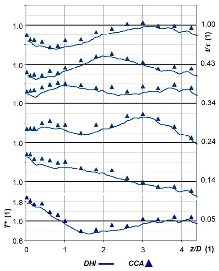
Figure 6.
Axis temperature development, depending on the distance from the actuator orifice; curves correspond to DHI and triangles to the CCA experiments; the DHI results are obtained as mean values along the z-axis. The CCA results are measured at z = 0.
4.2. DHI Validation of the Tomographic Measurement of the 3D Temperature Field by DHI Steady Flow
The measurement of steady flow is not as complex as the measurement of dynamic phenomena, and it can easily reveal weak points of the tomographical approach. Therefore, steady flow was used for the first experimental validation of the method. A non-symmetrical temperature field of heated air flowing out from a three-orifice system was measured (Figure 7a). As a reference, DHI results were compared to well-characterized and traceable CCA (constant current anemometry) measurements. CCA is a one-point method, and therefore, we have selected several representative points within the measured area. CCA measurements were performed along horizontal lines at different heights. The results at different heights (5 mm, 10 mm, 20 mm, and 40 mm) are denoted by the letters A–D, and these are shown in Figure 7b. The distance of the CCA measurement step in the horizontal direction was 1 mm. DHI is the full-field method, so that voxels from the measured temperature distribution corresponding to the position of the measured CCA values were selected. 1D graphs marked A–D present the results obtained by DHI and CCA along the horizontal cuts, with the same position for both types of measurements. The root-mean-square deviation at all of the measured points was calculated to quantify the difference between the results obtained from both methods. The RMS value was 3.8 °C, which can be considered as a measurement match within a range of about 12%. The main contribution to the measured discrepancies in DHI and CCA results is probably the fact that both measurements had to be done separately at different times, due to the invasive features of CCA. Despite the inconsistencies mentioned, the consensus is good, and it can be stated that DHI provides comparable results as the established CCA.
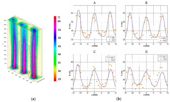
Figure 7.
(a) Tomographic reconstruction of the temperature field of steady flow, (b) temperature profiles measured over a distance of 5 mm (A), 10 mm (B), 20 mm (C), and 40 mm (D) from the orifices.
4.3. DHI Measurements of the Dynamic Asymmetrical Temperature Field—Synthetic Jets
In the previous section, it was verified that DHI is a reliable measurement method, and it can be used, e.g., for general (asymmetrical) periodic phenomena. This paragraph presents the results of the measurement of the 3D temperature field of two synthetic jet systems operating at 8 Hz; see Figure 8.
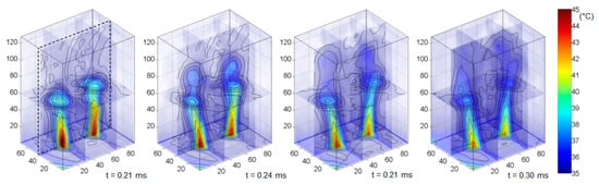
Figure 8.
A tomographically reconstructed 3D temperature field of SJ, measured over different times. The period of SJ was set to τ = 125 ms.
Assuming a periodic phenomenon, the averaging of many phase (or temperature) fields corresponding to the same relative time of the SJ period (see Figure 4), results in the suppression of the signal fluctuation (random) component. The fluctuation component, expressed as a ratio R of a standard deviation of the measured phase sequence to its mean value, is shown in Figure 9.

Figure 9.
The fluctuation component R, representing the amount of random fluctuations of the SJ.
The value of R is calculated in each pixel (m, n) as:
where and N is the number of averaged phases (N = 20 in our case). The fluctuation component of the temperature field described by the standard deviation is less than 17%. For the measurement, it is assumed to be a coherence of the phenomena. The fluctuation map represents the correlation of the temperature distribution between different periods. The fluctuation map for a fully coherent phenomenon would approach zero, while for stochastic temperatures, the field goes to 1.
5. Conclusions
The paper presents the possibilities for using digital holographic interferometry for the measurement of temperature field distribution generated by SJ actuators. A Twyman–Green interferometer with double sensitivity was used. Due to the synchronization between the camera external trigger and the actuator driver (resulting in the “freezing” of the SJ at certain time instants), periodic SJs of high frequencies can be measured with a low-frame-rate digital camera. Two different approaches were introduced: a 2D measurement mode and a 3D mode. The 2D mode enables the measurement of the average temperature along the optical axis, and one measurement projection is sufficient. On the other hand, the 3D temperature field distribution measurement requires measurements from different projections. The 3D measurement is based on the tomographic approach, and data from different projections are captured with the use of only one precisely synchronized camera with the SJ actuator driver.
The DHI experiments and tomography reconstruction experiments are performed on two kinds of SJ actuators: (a) with one emitting orifice, (b) with two emitting orifices.
In the case of 2D digital holographic interferometry, the results are compared with the results of the CCA method.
The temperature field of the fluid generated by the SJ actuator comprises three components, mean, periodic, and random fluctuation. It was measured that ratio of the random fluctuation to the periodic component was less than 17%.
The measurement time strongly depends on the number of projections. When rotating the object, there are a few seconds for the movement, and 2 s, in order to allow the system to mechanically settle down. The time required for capturing a sequence of holograms for one projection is below 2 s. For 90 projections, the total measurement time is approximately 6 min. The time could be decreased by a factor of 2 by using a more robust rotary stage and a camera of higher frame rate.
Author Contributions
Conceptualization, P.D., P.P., and T.V.; Funding acquisition, T.V.; Investigation, P.D. and P.P.; Methodology, P.D., P.P., and T.V.; Project administration, T.V.; Writing—original draft, P.D. and P.P.
Funding
We gratefully acknowledge the support of the Grant Agency CR (project No. 16-16596S).
Conflicts of Interest
The authors declare no conflict of interest.
References
- Liu, S.; Sakr, M. A comprehensive review on passive heat transfer enhancements in pipe exchangers. Renew. Sustain. Energy Rev. 2013, 19, 64–81. [Google Scholar] [CrossRef]
- Vasiliev, L.L. Heat pipes in modern heat exchangers. Appl. Therm. Eng. 2005, 25, 1–19. [Google Scholar] [CrossRef]
- Straka, P.; Prihoda, J.; Kozisek, M.; Furst, J. Simulation of transitional flows through a turbine blade cascade with heat transfer for various flow conditions. Eur. Phys. J. Conf. 2017, 143, 02118. [Google Scholar] [CrossRef]
- Verstraete, T.; Alsalihi, Z.; Van den Braembussche, R.A. Numerical Study of the Heat Transfer in Micro Gas Turbines. J. Turbomach. 2006, 129, 835–841. [Google Scholar] [CrossRef]
- Xiao, G.; Yang, T.; Liu, H.; Ni, D.; Ferrari, M.L.; Li, M.; Luo, Z.; Cen, K.; Ni, M. Recuperators for micro gas turbines: A review. Appl. Energy 2017, 197, 83–99. [Google Scholar] [CrossRef]
- Verstraete, D.; Bowkett, C. Impact of heat transfer on the performance of micro gas turbines. Appl. Energy 2015, 138, 445–449. [Google Scholar] [CrossRef]
- Hasnain, S.M. Review on sustainable thermal energy storage technologies, Part I: Heat storage materials and techniques. Energy Convers. Manag. 1998, 39, 1127–1138. [Google Scholar] [CrossRef]
- Hanchen, M.; Brückner, S.; Steinfeld, A. High-temperature thermal storage using a packed bed of rocks—Heat transfer analysis and experimental validation. Appl. Therm. Eng. 2011, 31, 1798–1806. [Google Scholar] [CrossRef]
- Agyenim, F.; Hewitt, N.; Eames, P.; Smyth, M. A review of materials, heat transfer and phase change problem formulation for latent heat thermal energy storage systems. Renew. Sustain. Energy Rev. 2010, 14, 615–628. [Google Scholar] [CrossRef]
- Krishnamurthy, M.R.; Prasannakumara, B.C.; Gireesha, B.J.; Gorla, R.S.R. Effect of chemical reaction on MHD boundary layer flow and melting heat transfer of Williamson nanofluid in porous medium. Eng. Sci. Technol. Int. J. 2016, 19, 53–61. [Google Scholar] [CrossRef]
- Khan, W.A.; Irfan, M.; Khan, M.; Alshomrani, A.S.; Alzahrani, A.K.; Alghamdi, M.S. Impact of chemical processes on magneto nanoparticle for the generalized Burgers fluid. J. Mol. Liq. 2017, 234, 201–208. [Google Scholar] [CrossRef]
- Venkateswarlu, B.; Satya Narayana, P.V. Chemical reaction and radiation absorption effects on the flow and heat transfer of a nanofluid in a rotating system. Appl. Nanosci. 2015, 5, 351–360. [Google Scholar] [CrossRef]
- Zhao, J.; Huang, S.; Gong, L.; Huang, Z. Numerical study and optimizing on micro square pin-fin heat sink for electronic cooling. Appl. Therm. Eng. 2016, 93, 1347–1359. [Google Scholar] [CrossRef]
- Abdoli, A.; Jimenez, G.; Dulikravich, G.S. Thermo-fluid analysis of micro pin-fin array cooling configurations for high heat fluxes with a hot spot. Int. J. Therm. Sci. 2015, 90, 290–297. [Google Scholar] [CrossRef]
- Liu, D.; Zhao, F.Y.; Yang, H.X.; Tang, G.F. Thermoelectric mini cooler coupled with micro thermosiphon for CPU cooling system. Energy 2015, 83, 29–36. [Google Scholar] [CrossRef]
- Sohel Murshed, S.M.; Nieto de Castro, C.A. A critical review of traditional and emerging techniques and fluids for electronics cooling. Renew. Sustain. Energy Rev. 2017, 78, 821–833. [Google Scholar] [CrossRef]
- Dancova, P. Experimental Investigation of Synthetic Jets in a Laminar Channel Flow. Ph.D. Thesis, Technical University of Liberec, Liberec, Czech Republic, 2012. [Google Scholar]
- Dancova, P.; Travnicek, Z.; Vit, T. Experimental Investigation of a Synthetic Jet Array in a Laminar Channel Flow. Eur. Phys. J. Conf. 2013, 45, 01002. [Google Scholar] [CrossRef]
- Timchenko, V.; Reizes, J.A.; Leonardi, E. An Evaluation of Synthetic Jets for Heat Transfer Enhancement in Air Cooled Micro-Channels. Int. J. Numer. Methods Heat Fluid Flow 2007, 17, 263–283. [Google Scholar] [CrossRef]
- Travnicek, Z.; Dancova, P.; Lam, J.H.; Timchenko, V.; Reizes, J. Numerical and experimental studies of a channel flow with multiple circular synthetic jets. Eur. Phys. J. Conf. 2012, 25, 01094. [Google Scholar] [CrossRef]
- Chaudhari, M.; Puranik, B.; Agrawal, A. Multiple orifice synthetic jet for improvement in impingement heat transfer. Int. J. Heat Mass Transf. 2011, 54, 2056–2065. [Google Scholar] [CrossRef]
- Al-Asadi, M.T.; Alkasmoul, F.S.; Wilson, M.C.T. Heat transfer enhancement in a micro-channel cooling system using cylindrical vortex generators. Int. Commun. Heat Mass Transf. 2016, 74, 40–47. [Google Scholar] [CrossRef]
- Chen, C.; Teng, J.T.; Cheng, C.H.; Jin, S.; Huang, S.; Liu, C.; Lee, M.T.; Pan, H.H.; Greif, R. A study on fluid flow and heat transfer in rectangular microchannels with various longitudinal vortex generators. Int. J. Heat Mass Transf. 2014, 69, 203–214. [Google Scholar] [CrossRef]
- Al-Asadi, M.T.; Alkasmoul, F.S.; Wilson, M.C.T. Benefits of spanwise gaps in cylindrical vortex generators for conjugate heat transfer enhancement in micro-channels. Appl. Therm. Eng. 2018, 130, 571–586. [Google Scholar] [CrossRef]
- Smith, B.L.; Glezer, A. The formation and evolution of synthetic jets. Phys. Fluids 1998, 10, 2281–2297. [Google Scholar] [CrossRef]
- Holman, R.; Utturkar, Y. Formation Criterion for Synthetic Jets. AIAA J. 2005, 43, 2110–2116. [Google Scholar] [CrossRef]
- Cater, J.E.; Soria, J. The evolution of round zero-net-mass-flux jets. J. Fluid Mech. 2002, 472, 167–200. [Google Scholar] [CrossRef]
- Glezer, A.; Amitay, M. Synthetic jets. Annu. Rev. Fluid Mech. 2002, 34, 503–529. [Google Scholar] [CrossRef]
- Chiatto, M.; Capuano, F.; de Luca, L. Numerical and experimental characterization of a double-orifice synthetic jet actuator. Meccanica 2018, 53, 2883–2896. [Google Scholar] [CrossRef]
- Mallinson, S.G.; Reizes, J.A.; Hong, G.; Westbury, P.S. Analysis of hot-wire anemometry data obtained in a synthetic jet flow. Exp. Fluid Sci. 2004, 28, 265–272. [Google Scholar] [CrossRef]
- Bruun, H.H. Hot Wire Anemometry; Oxford Univ. Press: Oxford, NY, USA, 1995. [Google Scholar]
- Childs, P.R.N.; Greenwood, J.R.; Long, C.A. Review of temperature measurement. Rev. Sci. Instrum. 2000, 71, 2959–2978. [Google Scholar] [CrossRef]
- Hall, R.J.; Bonczyk, P.A. Sooting Flame Thermometry Using Emission/Absorption Tomography. Appl. Opt. 1990, 29, 4590–4598. [Google Scholar] [CrossRef]
- Kampmann, S.; Leipertz, A.; Döbbeling, K.; Haumann, J.; Sattelmayer, T. Two-dimensional temperature measurements in a technical combustor with laser Rayleigh scatterin. Appl. Opt. 1993, 32, 6167–6172. [Google Scholar] [CrossRef]
- Feldmann, O.; Mayinger, F. Optical Measurements—Techniques and Applications; Springer: Berlin, Germany, 2001. [Google Scholar]
- Dancova, P. Analysis of the “Synthetic Jet”. Master’s Thesis, Technical University of Liberec, Liberec, Czech Republic, 2006. [Google Scholar]
- Gabor, D. A new microscopic principle. Nature 1948, 161, 777–778. [Google Scholar] [CrossRef]
- Leith, E.N.; Upatnieks, J. Wavefront Reconstruction with Diffused Illumination and Three-Dimensional Objects. J. Opt. Soc. Am. 1964, 54, 1295. [Google Scholar] [CrossRef]
- Lohmann, A.W.; Paris, D.P. Binary Fraunhofer Holograms, Generated by Computer. Appl. Opt. 1967, 6, 1739. [Google Scholar] [CrossRef]
- Lee, W.H. Binary Synthetic Holograms. Appl. Opt. 1974, 13, 1677–1682. [Google Scholar] [CrossRef]
- Lee, W.H. Sampled Fourier Transform Hologram Generated by Computer. Appl. Opt. 1970, 9, 639–643. [Google Scholar] [CrossRef]
- Heanue, F.; Bashaw, M.C.; Hesselink, L. Volume holographic storage and retrieval of digital data. Science 1994, 265, 749–752. [Google Scholar] [CrossRef]
- Powell, R.L.; Stetson, K.A. Interferometric Vibration Analysis by Wavefront Reconstruction. J. Opt. Soc. Am. 1965, 55, 1593–1598. [Google Scholar] [CrossRef]
- Stetson, K.A.; Powell, R.L. Interferometric Hologram Evaluation and Real-Time Vibration Analysis of Diffuse Objects. J. Opt. Soc. Am. 1965, 55, 1694–1695. [Google Scholar] [CrossRef]
- Brooks, R.E.; Heflinger, L.O.; Wuerker, R.F. Interferometry with a Holographically Reconstructed Comparison Beam. Appl. Phys. Lett. 1965, 7, 248–249. [Google Scholar] [CrossRef]
- Haines, K.A.; Hildebrand, B.P. Surface-Deformation Measurement using the Wavefront Reconstruction Technique. Appl. Opt. 1966, 5, 595–602. [Google Scholar] [CrossRef] [PubMed]
- Hildebrand, B.P.; Haines, K.A. The generation of three-dimensional contour maps by wavefront reconstruction. Phys. Lett. 1966, 21, 422–423. [Google Scholar] [CrossRef]
- Heflinger, L.O.; Wuerker, R.F. Holographic Contouring via Multifrequency Lasers. Appl. Phys. Lett. 1969, 15, 28–30. [Google Scholar] [CrossRef]
- Horman, M.H. An Application of Wavefront Reconstruction to Interferometry. Appl. Opt. 1965, 4, 333–336. [Google Scholar] [CrossRef]
- Sweeney, D.W.; Vest, C.M. Reconstruction of Three-Dimensional Refractive Index Fields from Multidirectional Interferometric Data. Appl. Opt. 1973, 12, 2649–2664. [Google Scholar] [CrossRef] [PubMed]
- Lira, I.H.; Vest, C.M. Refraction correction in holographic interferometry and tomography of transparent objects. Appl. Opt. 1987, 26, 3919–3928. [Google Scholar] [CrossRef]
- Goodman, J.W.; Lawrence, R.W. Digital Image Formation from Electronically Detected Holograms. Appl. Phys. Lett. 1967, 11, 176–181. [Google Scholar] [CrossRef]
- Kronrod, M.A.; Yaroslavsky, L.P.; Merzlyakov, N.S. Reconstruction of holograms with a computer. Sov. Phys. Technol. Phys. 1972, 17, 333–334. [Google Scholar]
- Schnars, U.; Jüptner, W. Direct recording of holograms by a CCD target and numerical reconstruction. Appl. Opt. 1994, 33, 179–181. [Google Scholar] [CrossRef]
- Zou, Y.; Pedrini, G.; Tiziani, H. Surface contouring in a video frame by changing the wavelength of a diode laser. Opt. Eng. 1996, 35, 1074–1079. [Google Scholar] [CrossRef]
- Kreis, T. Handbook of Holographic Interferometry, Optical and Digital Methods; Wiley: Berlin, Germany, 2004. [Google Scholar]
- Schnars, U.; Jueptner, W. Digital Holography: Digital Hologram Recording, Numerical Reconstruction, and Related Techniques; Springer: Berlin, Germany, 2004. [Google Scholar]
- Kim, M.K. Principles and techniques of digital holographic microscopy. J. Photonics Energy 2010, 1, 18005. [Google Scholar] [CrossRef]
- Garcia-Sucerquia, J.; Xu, W.; Jericho, S.K.; Klages, P.; Jericho, M.H.; Kreuzer, H.J. Digital in-line holographic microscopy. Appl. Opt. 2006, 45, 836–850. [Google Scholar] [CrossRef] [PubMed]
- Takaki, Y.; Ohzu, H. Fast Numerical Reconstruction Technique for High-Resolution Hybrid Holographic Microscopy. Appl. Opt. 1999, 38, 2204–2211. [Google Scholar] [CrossRef] [PubMed]
- Dubois, F.; Joannes, L.; Legros, J.C. Improved Three-Dimensional Imaging with a Digital Holography Microscope with a Source of Partial Spatial Coherence. Appl. Opt. 1999, 38, 7085–7094. [Google Scholar] [CrossRef] [PubMed]
- Vit, T.; Ledl, V.; Dolecek, R.; Psota, P. The Possibility of Visualizing Temperature Fields Using Digital Holographic Interferometry. Appl. Mech. Mater. 2013, 284, 988–995. [Google Scholar] [CrossRef]
- Ledl, V.; Vit, T.; Dolecek, R.; Psota, P. Digital holographic interferometry used for identification of 2D temperature field. Eur. Phys. J. Conf. 2012, 25, 02014. [Google Scholar] [CrossRef]
- Dolecek, R.; Psota, P.; Ledl, V.; Vit, T.; Václavik, J.; Kopecky, V. General temperature field measurement by digital holography. Appl. Opt. 2013, 52, A319–A325. [Google Scholar] [CrossRef] [PubMed]
- Dancova, P.; Vit, T.; Ledl, V.; Travnicek, Z.; Dolecek, R. Holographic interferometry as a tool for visualization of temperature fields in air. Eng. Mech. 2013, 20, 205–212. [Google Scholar]
- Ledl, V.; Psota, P.; Dolecek, R.; Vit, T. Digital holographic setups for phase object measurements in micro and macro scale. Eur. Phys. J. Conf. 2015, 92, 01001. [Google Scholar] [CrossRef]
- Dancova, P.; Dolecek, R.; Ledl, V. Experimental investigation of temperature fields in a synthetic jet. MATEC Web Conf. 2014, 18, 03001. [Google Scholar] [CrossRef]
© 2019 by the authors. Licensee MDPI, Basel, Switzerland. This article is an open access article distributed under the terms and conditions of the Creative Commons Attribution (CC BY) license (http://creativecommons.org/licenses/by/4.0/).