Article

Stabilization of Magnetic Suspension System by Using Only a First-Order Reset Element without a Derivative Element

Department of Mechanical Engineering, Saitama University, Shimo okubo 255, Sakura-ku, Saitama 338-8570, Japan
*
Author to whom correspondence should be addressed.
Actuators 2019, 8(1), 24; https://doi.org/10.3390/act8010024
Submission received: 31 January 2019 / Revised: 28 February 2019 / Accepted: 6 March 2019 / Published: 9 March 2019
(This article belongs to the Special Issue Magnetic Bearing Actuators)

Abstract

:
The stabilization of a magnetic suspension system is achieved by using a low-pass filter (LPF) with a nonlinear integrator without any other element. A proportional-derivative (PD) control is commonly used as the simplest method of stabilizing a magnetic suspension system. Meanwhile, a first-order reset element (FORE) was applied to improve transient characteristics. The original FORE was a first-order LPF with a nonlinear reset integrator element. A magnetic suspension system cannot be stabilized by a linear LPF, nor the original FORE. In this work, the reset conditions of the FORE were modified for magnetic suspension. This modified FORE succeeded in stabilizing a magnetic suspension system. The efficacy of the modified FORE was demonstrated by simulations and experiments. A single degree of freedom magnetic suspension system was used in the experiment.

1. Introduction

A magnetic suspension system without a control is unstable and undamped. A proportional-derivative (PD) control is the simplest control method of stabilizing a magnetic suspension system. Using a PD controller, restoring force is produced with the proportional element, and damping is produced with the derivative element. Meanwhile, installing a reset element in the control system has been used for a long time. The reset system [1] is a hybrid system that combines continuous linear operation and partial discontinuous transition in certain conditions. The original reset control system goes back to 1958 with the work of Clegg [2]. He used a nonlinear integrator whose output was reset to zero when the input to the integrator crossed zero. Clegg’s integrator (CI) is used solely or combined with other control elements, such as a proportional-integralcontroller [3,4]. Then, a first-order reset element (FORE) was proposed for the improvement of transient characteristics in 1975 [5]. The FORE was a first-order low-pass filter (LPF) with a nonlinear integrator with a reset function [6]. The FORE controller has been analyzed and studied recently [7,8]. Moreover, FORE controllers have been applied to various control objects, such as vibration reduction in a combustor [9], position regulation of an exhaust gas recirculation valve [10], active suspension control [11], unmanned aerial vehicle control [12], and piezo-actuated motion control [13]. In this work, the FORE control was applied to active magnetic suspension. The magnetic suspension system is unstable and undamped. It cannot be stabilized by a single linear first-order LPF, nor the original FORE. The reset conditions of the FORE were modified to stabilize the magnetic suspension system. The efficacy of the modified FORE in magnetic suspension was demonstrated through simulations and experiments.

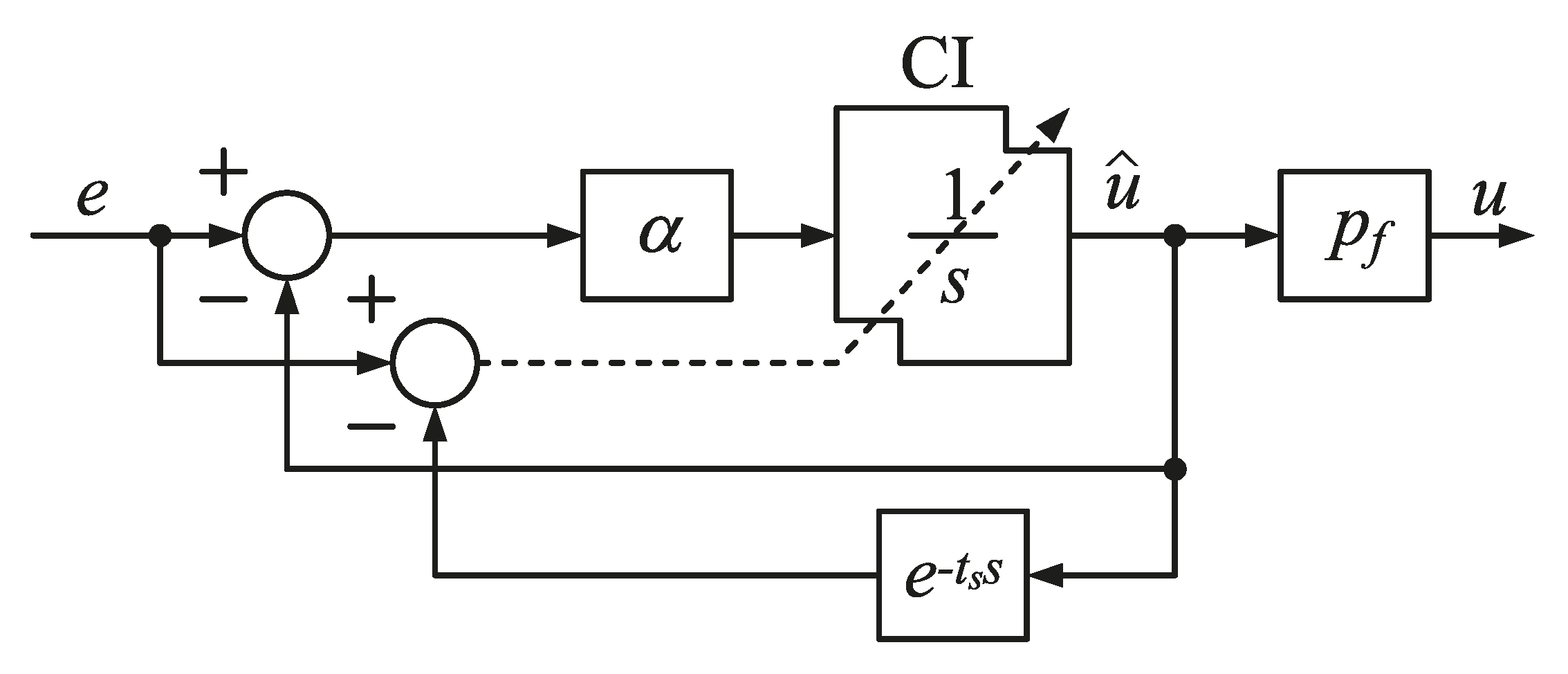
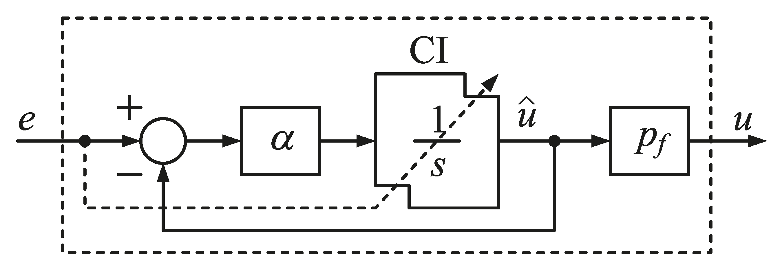
2. First-Order Reset Element

2.1. Original FORE

A block diagram of the original FORE is shown in Figure 1. The FORE is a first-order LPF using CI instead of a standard linear integrator. The reset controller is customarily represented with a broken box. The broken box in Figure 1 represents CI. The signal to be integrated is represented with an arrowed solid line. This signal is the difference between the input of the FORE (e) and the output of the CI (û), multiplied by the factor α that determines the cutoff angular frequency of the low-pass filter. The allowed dashed line represents the reset terminal of the CI. The reset terminal is connected to the input of the FORE. The output of the CI is reset to zero when the input of the FORE crosses zero. The output of the FORE (u) is the product of the output of the CI (û) and the gain (pf).
The base linear system C(s), which represents the underlying continuous mode of operation in the FORE, is represented by
C ( s ) = p f α s + α .
The reset conditions of the CI used in the original FORE are expressed by
{ u ^ ˙ ( t ) = α ( e ( t ) u ^ ( t ) ) u ^ ( t + ) = 0 : e ( t ) 0 : e ( t ) = 0 .
The FORE can make vibrations attenuate faster than linear LPF [1]. However, the original FORE cannot stabilize a magnetic suspension system. In this work, the reset conditions of the FORE were modified to stabilize the magnetic suspension system.

2.2. Modified FORE

Figure 2 shows a modified FORE for active magnetic suspension. The reset conditions of the modified FORE were defined based on the difference between the output signal of the CI and the input signal. A delay element was introduced for actual implementation because the controller without the delay element had an algebraic loop that made the implementation impossible with a digital controller.
The reset conditions of the CI used in the modified FORE are expressed by
{ u ^ ˙ ( t ) = α ( e ( t ) u ^ ( t ) ) u ^ ( t + ) = 0 : e ( t ) u ^ ( t t s ) 0 : e ( t ) u ^ ( t t s ) = 0 ,
where ts is the time delay due to the sampling time of the digital controller.

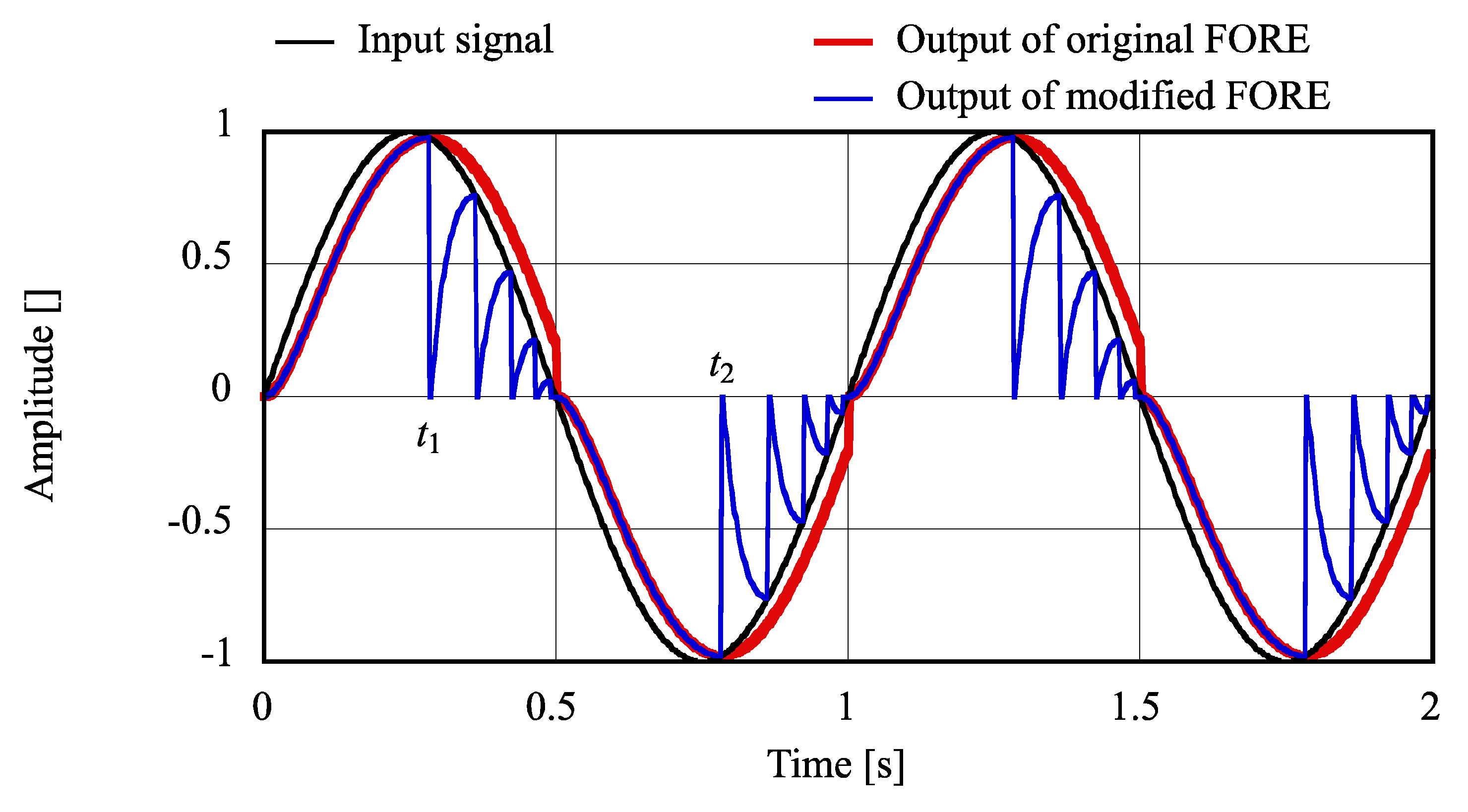
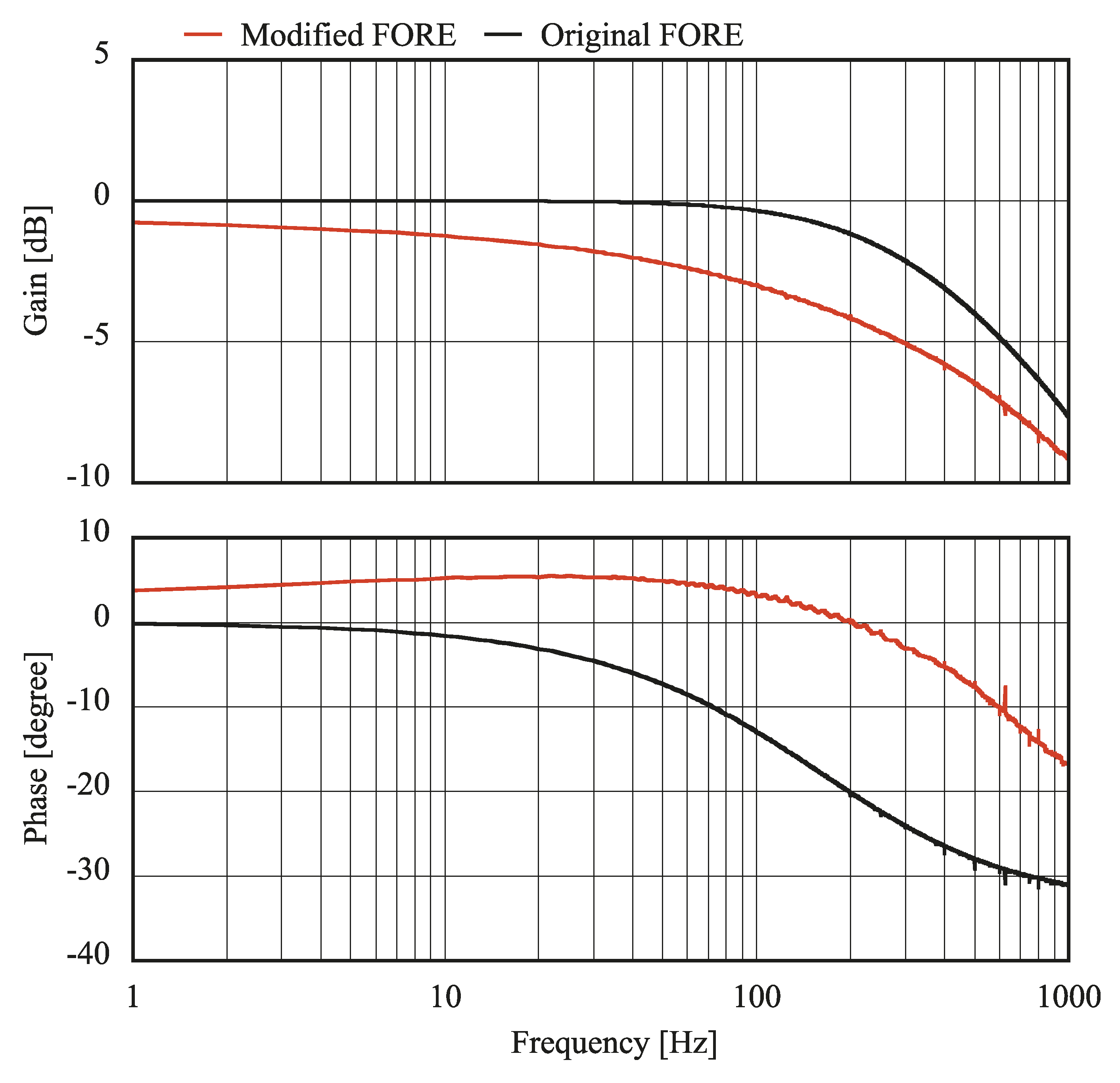
2.3. Comparison between Original and Modified FOREs through Simulations

The simulated time histories of the original and modified FORE outputs to a sinusoidal input are shown by Figure 3. In both FOREs, α = 30 rad/s and pf = 1. The inputted sinusoidal signal wave had a frequency of 1 Hz and an amplitude of 1. Both FOREs had the same output as that of the linear first-order LPF before the resets. The original FORE reset the output to zero when the input signal crossed zero (t = 0.5 s). The output signal of the modified FORE was reset to zero when the input signal crossed the unit-delayed output signal at t1. The reset actions were repeated until t = 0.5 s in the modified FORE. After t = 0.5 s, the output signals were the same as those of the first-order LPF again. The reset actions were repeated after t2 in the modified FORE, while the second reset occurred at t = 1 s in the original FORE. Figure 4 shows the frequency characteristics of both FOREs, with α = 2000 rad/s and pf = 1. They were calculated by using a Fourier transformation of the input and the output signals at each frequency. The original FORE was almost the same in gain as the first-order LPF. The gain of the modified FORE was smaller than them. The original FORE had a lag element characteristic in phase. The phase of the modified FORE led in the low-frequency region. Therefore, the modified FORE was effective, as expected, in stabilizing an undamped system.

3. Magnetic Suspension System

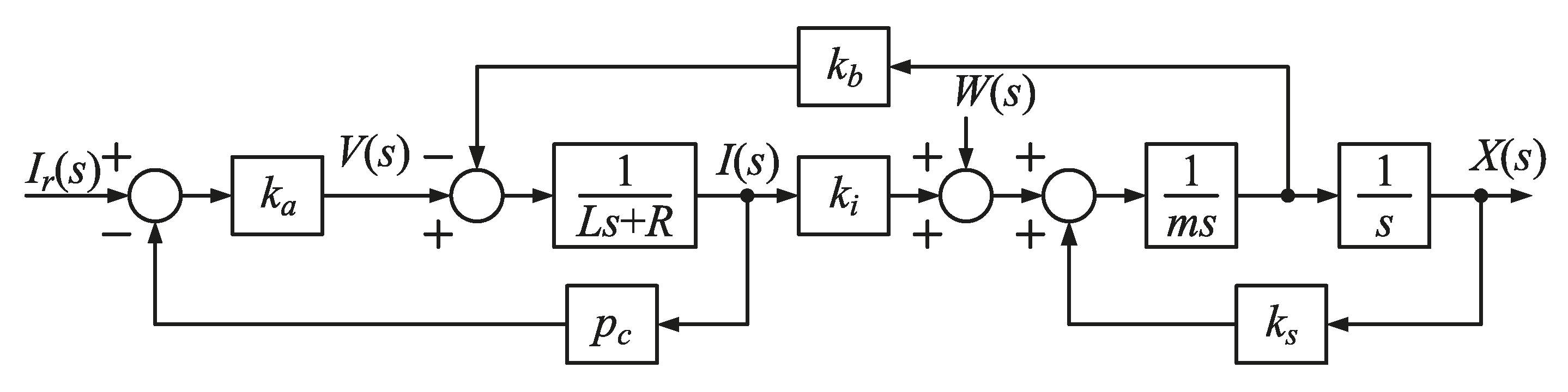
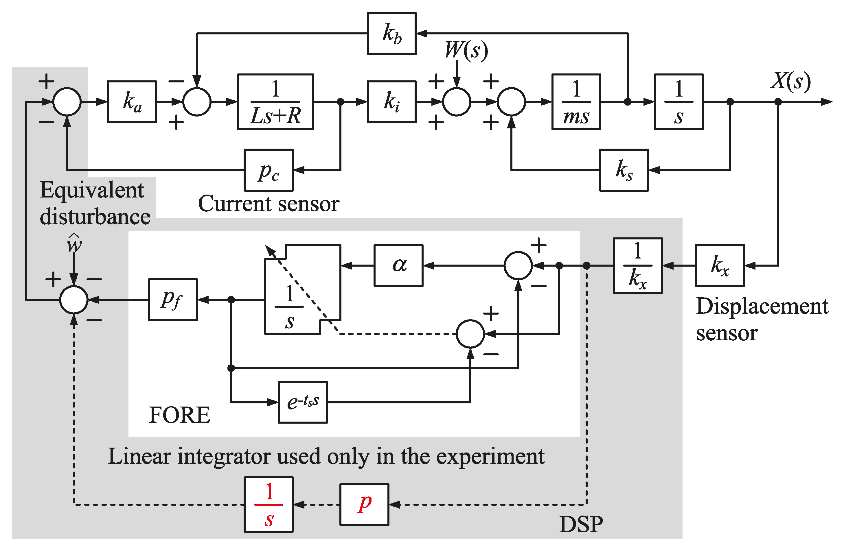
3.1. Model of Magnetic Suspension System

Figure 5 shows a photograph of a single degree of freedom magnetic suspension apparatus and the schematic motion of the floator. The size of the apparatus was approximately 320 × 200 × 110 mm. The electromagnet was attached to the top of the aluminum frame. The electromagnet had four coils and five poles. A suspended object (floator) had a magnetic target, an aluminum body connecting to the links, and a target of a displacement sensor. The core of the electromagnet and the magnetic target of the floator were made of soft iron. Figure 6 shows a schematic view of the electromagnet and the floator. The electromagnet had four coils and five core poles. The size of the electromagnet core was 40 × 70 × 70 mm. The floator was a disk shape with a diameter of 100 mm and a thickness of 10 mm. A disk permanent magnet was attached to the floator. The size of the permanent magnets was a diameter of 20 mm and a thickness of 1 mm. In this paper, the magnetic circuit consisted of the electromagnet, the floator target and the permanent magnet is called a hybrid electromagnet. The motion of the floator was restricted to a single degree of freedom motion in the gravitational direction by links and bearings. The friction in the bearings was rather small. Therefore, the floator vibrated when only the linear proportional feedback was applied with enough gain to produce a restoring force. The gap was in the distance between the surface of the electromagnet and the permanent magnet on the floator. Because the motion of the floator was limited mechanically, the gap could change from 6 mm to 13 mm. A counterbalancer was attached to the link mechanism. The forces acting on the floator were the attractive force generated by the hybrid magnet (upward), the gravitational force due to the mass of the floator (downward), and the gravitational force generated by the counterbalancer (upward). The forces acting in the vertical were balanced near the center of the gap with no current in the electromagnet.
Now, a model linearized around the equilibrium states will be derived. The equation of motion is given by [14]
m x ¨ = F + ( m b m ) g + w ,
where F is the attractive force produced by the hybrid magnet, x is the floator displacement from the equilibrium position, m is the mass of the floator, mb is the equivalent mass of the counterbalance, g is the acceleration due to gravity, and w is the disturbance force acting on the floator.
The attractive force of the hybrid magnet and gravity forces are assumed to be balanced at the equilibrium position. Then, the linearized equation is derived as
m x ¨ = k i i + k s x + w ,
where ki is the current-force coefficient of the hybrid magnet, i is the current flowing through the coil, and ks is the gap-force coefficient of the hybrid magnet.
The electrical circuit equation associated with the electromagnet becomes
L d i d t + R i + k b x ˙ = v ,
where L is the inductance of the coil, R is the resistance of the coil, kb is the velocity-voltage coefficient, and v is the voltage applied to the coil.
Figure 7 shows a block diagram of the control object. When each Laplace-transformed variable is denoted by its capital, and the initial values are assumed to be zero for simplicity, the transfer function representation of the dynamics described by Equations (9) and (10) becomes
X ( s ) = 1 m s 2 k s ( k i I ( s ) + W ( s ) ) ,
( L s + R ) I ( s ) + k b s X ( s ) = V ( s ) .
The magnetic suspension system could be classified into a voltage-control type and a current-control type according to the power amplifier [14]. The current-controlled magnetic suspension system was designed based on Equation (10). The voltage-controlled magnetic suspension system was designed based on Equations (10) and (11). In this paper, the voltage-controlled magnetic suspension system was treated. The input voltage to the power amplifier is given by the difference between the output voltage of the controller and the voltage of the current sensor. The output voltage of the power amplifier is given by
V ( s ) = k a ( I r ( s ) p c I ( s ) ) ,
where ka is the gain of the power amplifier, ir is the input to the amplifier, and pc is the gain of the current sensor.
Summarizing these equations leads to the following equation,
X ( s ) = 1 ( m s 2 k s ) ( L s + R + k a p c ) + k b k i s ( k a k i I r ( s ) + ( L s + R + k a p c ) W ( s ) ) .
The electrical parameters of the hybrid magnet were a resistance of 5.56 Ω and an inductance of 13.2 mH when an alternating current signal with a frequency of 100 Hz was applied. The parameter ki was calculated from the coil current when gravitational force was added to the floator with the proportional-integral-derivative control. The parameter ks was calculated from the displacement of the floator when the zero power control was applied. The mass of m was calculated from the relationship between the resonant frequency of the PD controlled system and the stiffness produced by the proportional feedback gain. The parameter kb was estimated from the generated counterelectromotive force when the floator was moved:
m = 1.2   kg , k s = 3000   N / m , k i = 3.6   N / A , k b = 4.5   Vs / m .

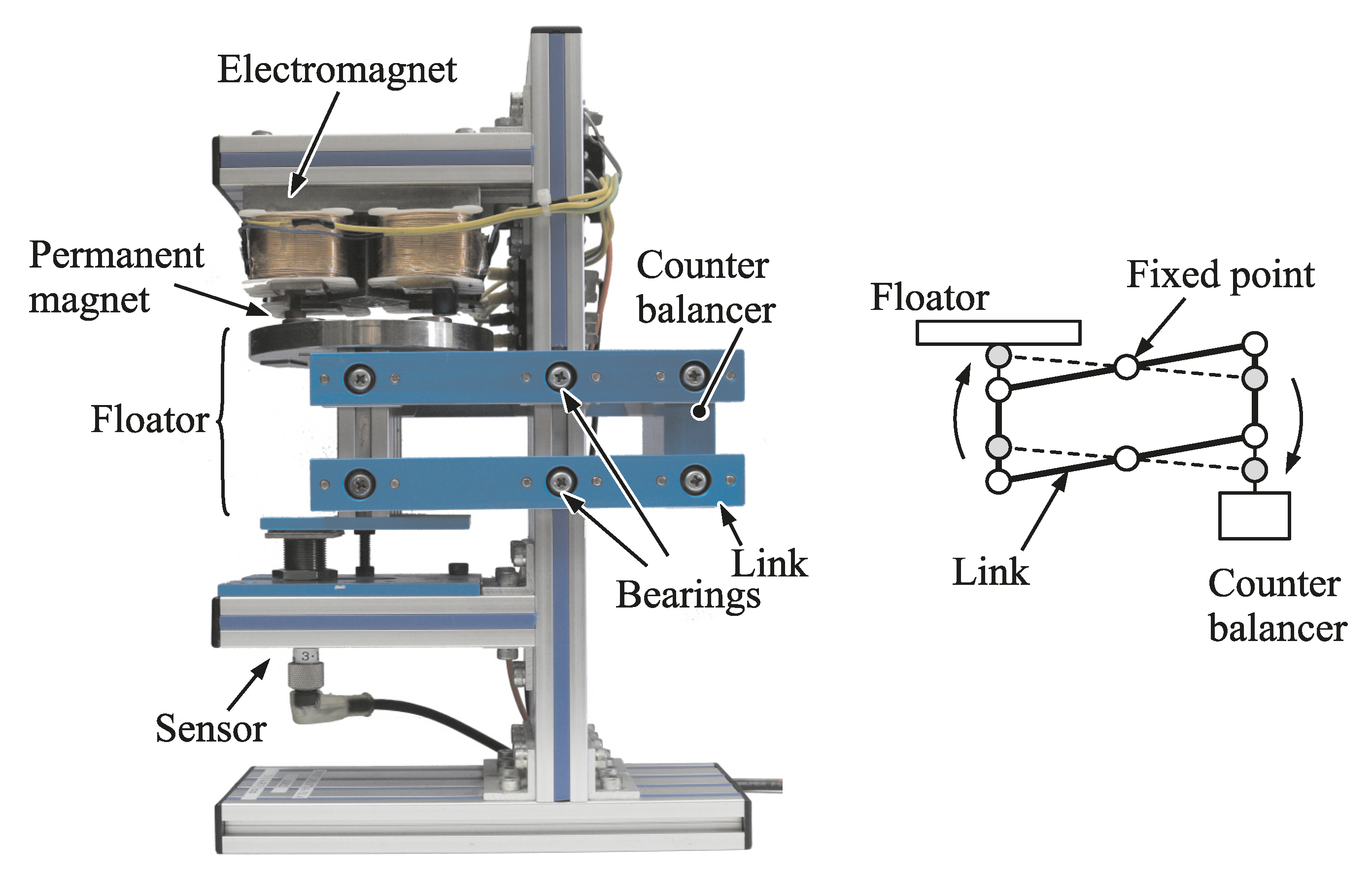
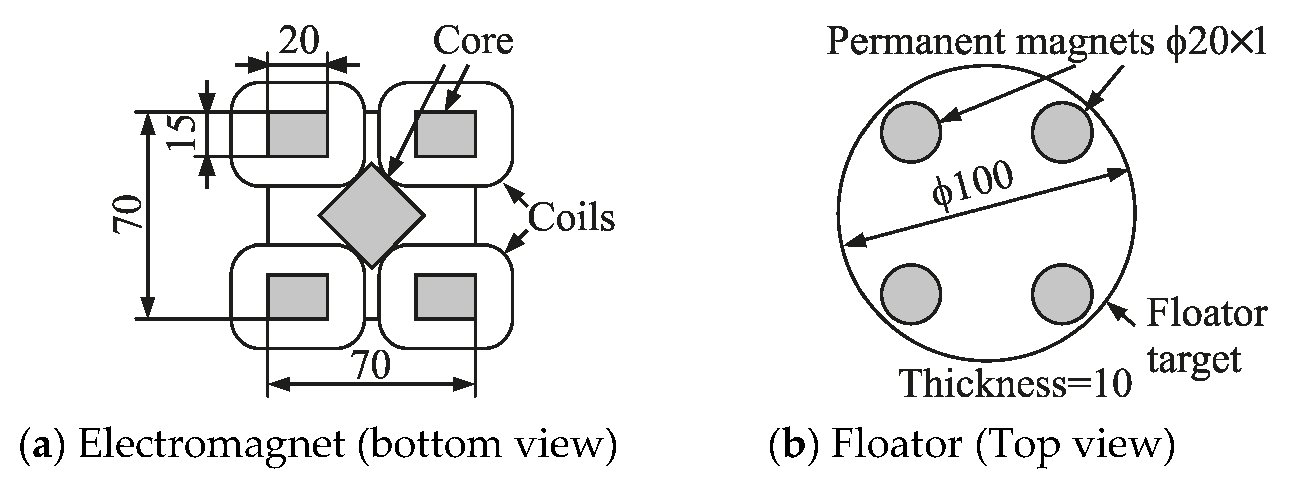
3.2. Experimental Setup

Figure 8 shows a block diagram of the experimental setup. The designed control algorithm was implemented with a DSP-based digital controller (DS-1005 made by dSPACE Ltd, Paderborn, Germany). The inside of the gray area in the figure represents the controller. The control period was set to 50 μs. The current of the coil was used as a feedback signal to the power amplifier via the controller. The gain of the current sensor pc was 1 V/A. In the experiment, disturbance was generated in the controller. It is represented by ŵ. When the gain ka was set to be large, the amplifier operated as a current output type. Then, ŵ could be treated as an equivalent disturbance force. The dimension of ŵ was converted to newtons by multiplying ki.
A linear integrator element was inserted parallel to the FORE in the experiment. The parameters varied from the nominal values in the experiment when the gap changed. In the actual system, an offset existed in the displacement sensor signal. Therefore, the steady-state position changed according to the feedback gain. To avoid such a change, a linear integrator was introduced to keep the steady-state gap constant. The gain of the integrator p was set to be small enough not to affect the transient responses. The amplifier was BWS60-5, provided by Takasago Ltd (Tokyo, Japan). The maximum rated voltage was ±60 V. The output current was limited between ±4 A to prevent the electromagnet from overheating. In voltage control mode, the gain of the amplifier was set to be 10 V/V. The gain of ka of the amplifier in Figure 8 included the gain multiplied in the controller. The current of the electromagnet was measured with a current sensor. The measured current was used as a feedback signal. The displacement of the floator was measured by an eddy current displacement sensor. The resolution of the displacement sensor was 5μm. The gain of the sensor kx was 3.30 V/mm.

4. Simulation Results

This section shows several simulation results. MATLAB and SIMULINK were used for the simulations. In the following simulations, the value of each parameter was set to be the same as that in the experiment. Unless otherwise specified, the feedback parameters and the cutoff angular frequency used in the simulation are given by
α = 2000   rad / s , p f = 2000   V / m , k a = 20   V / V .

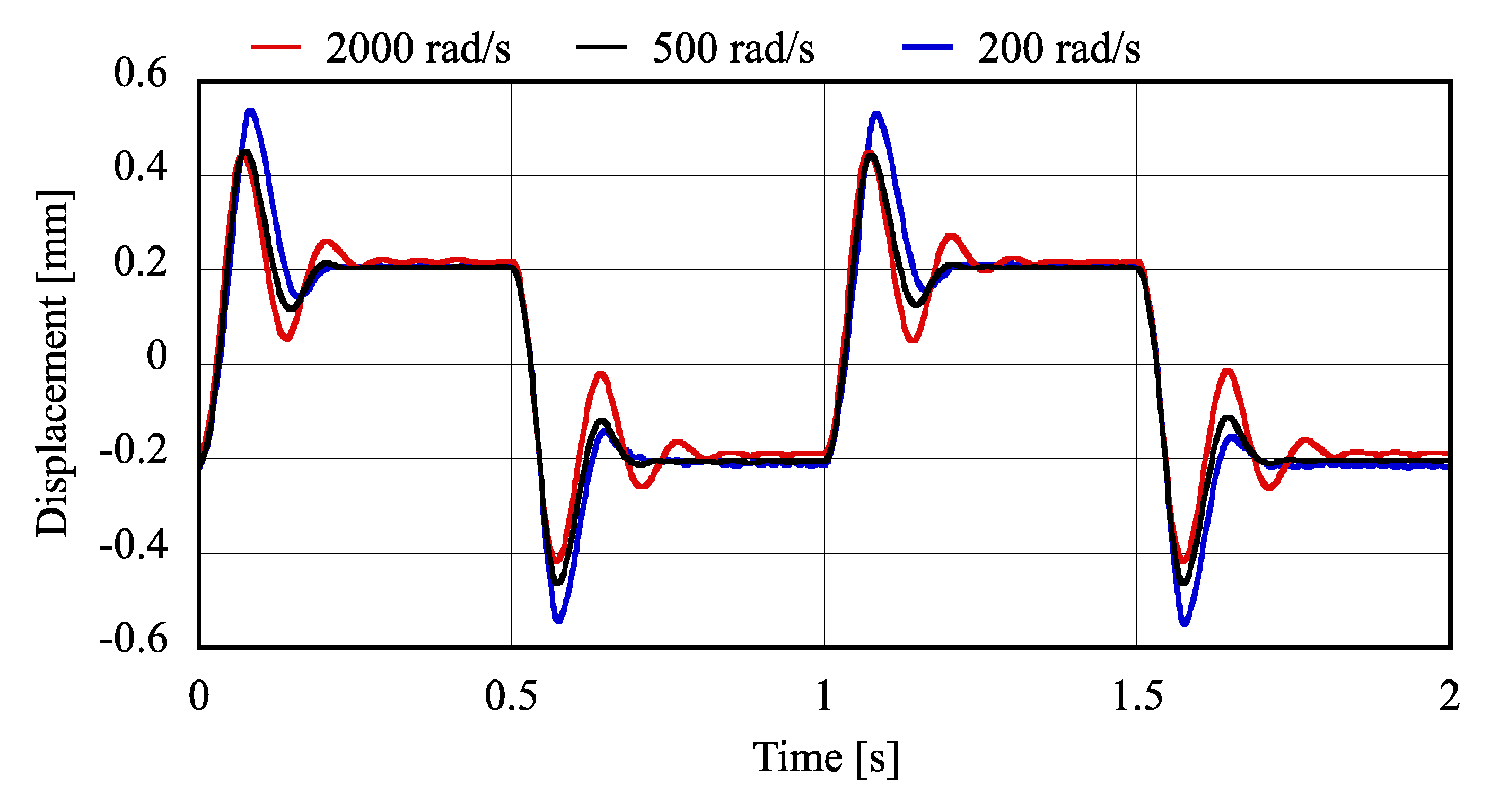
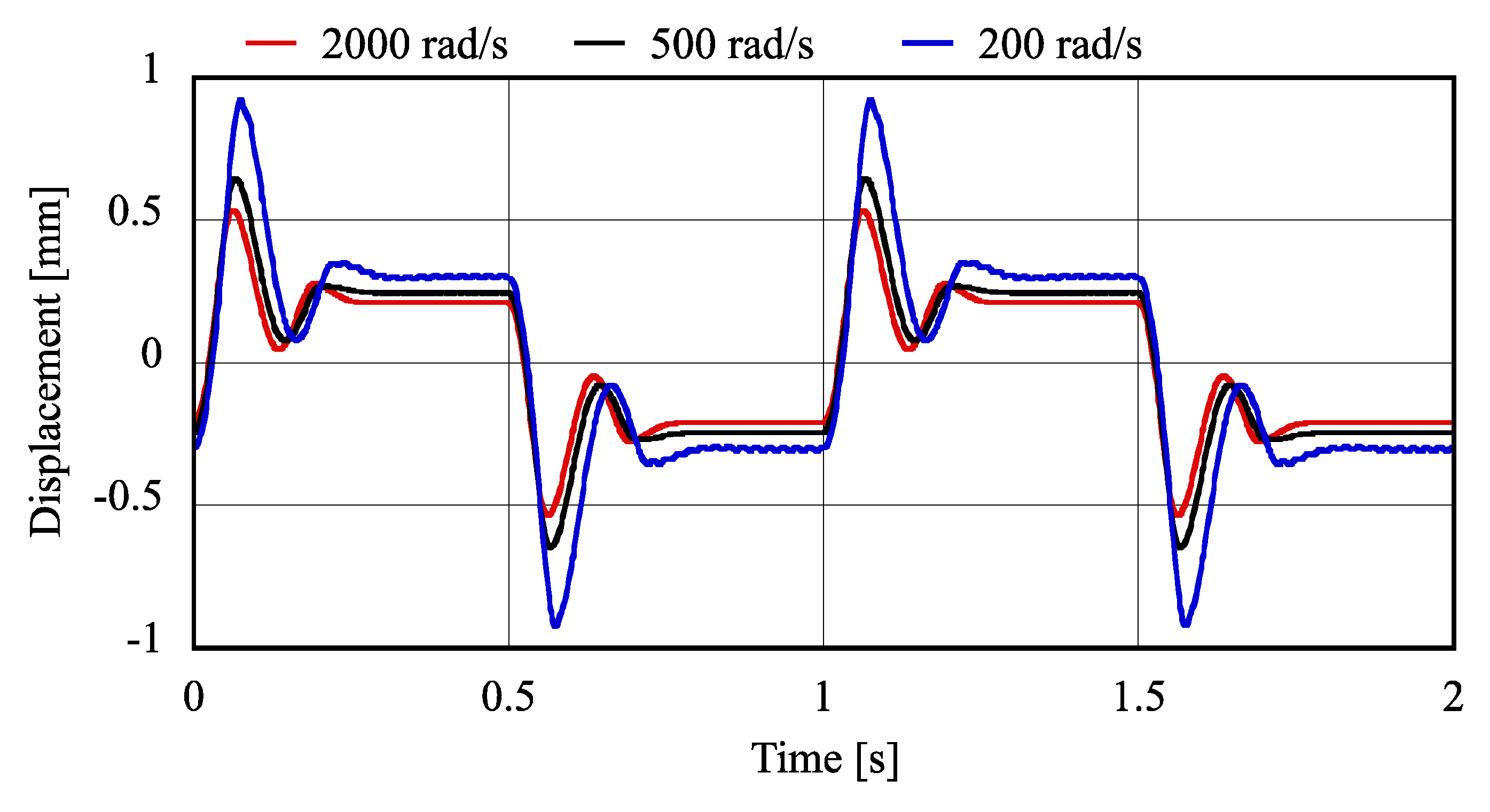
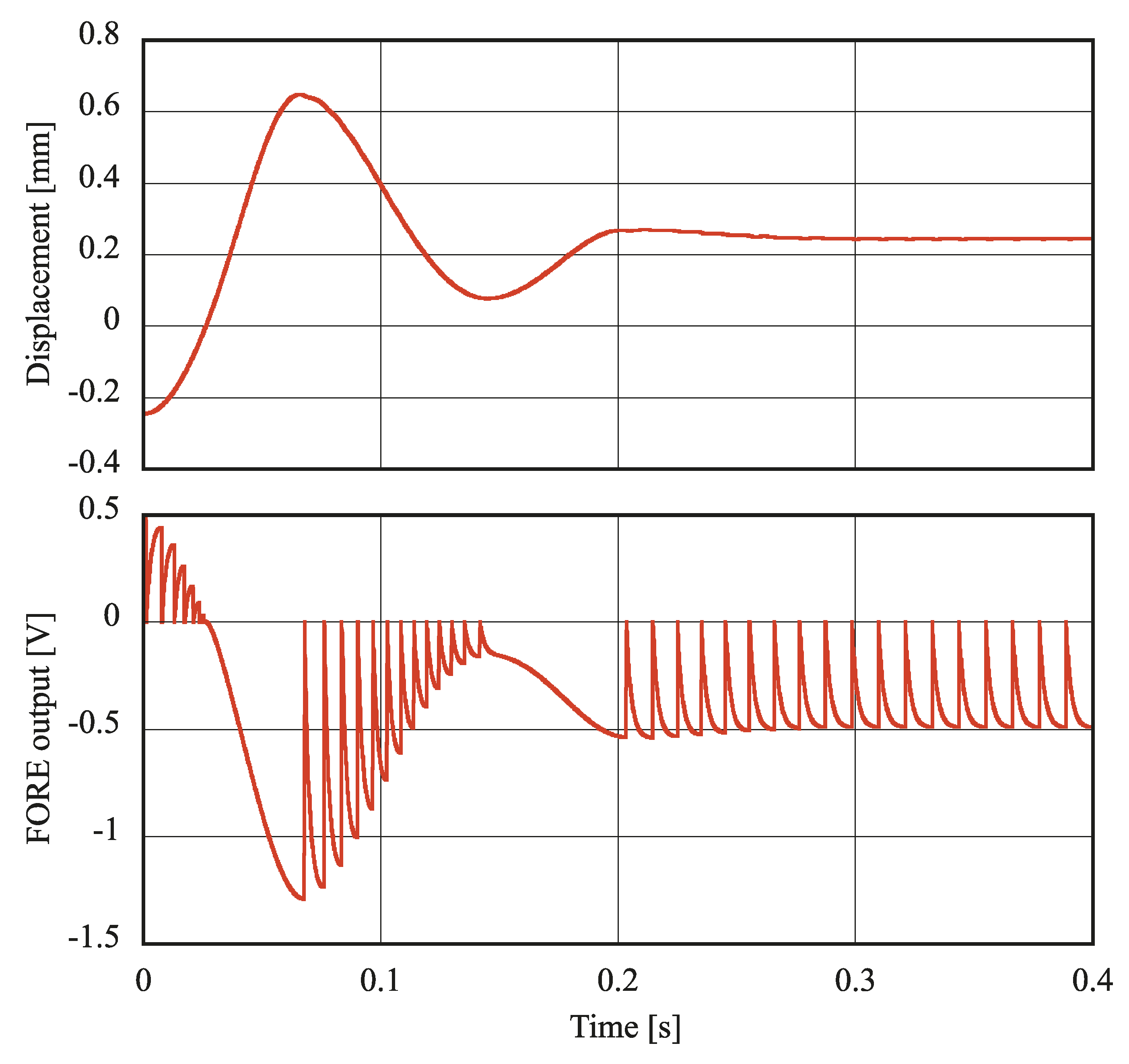
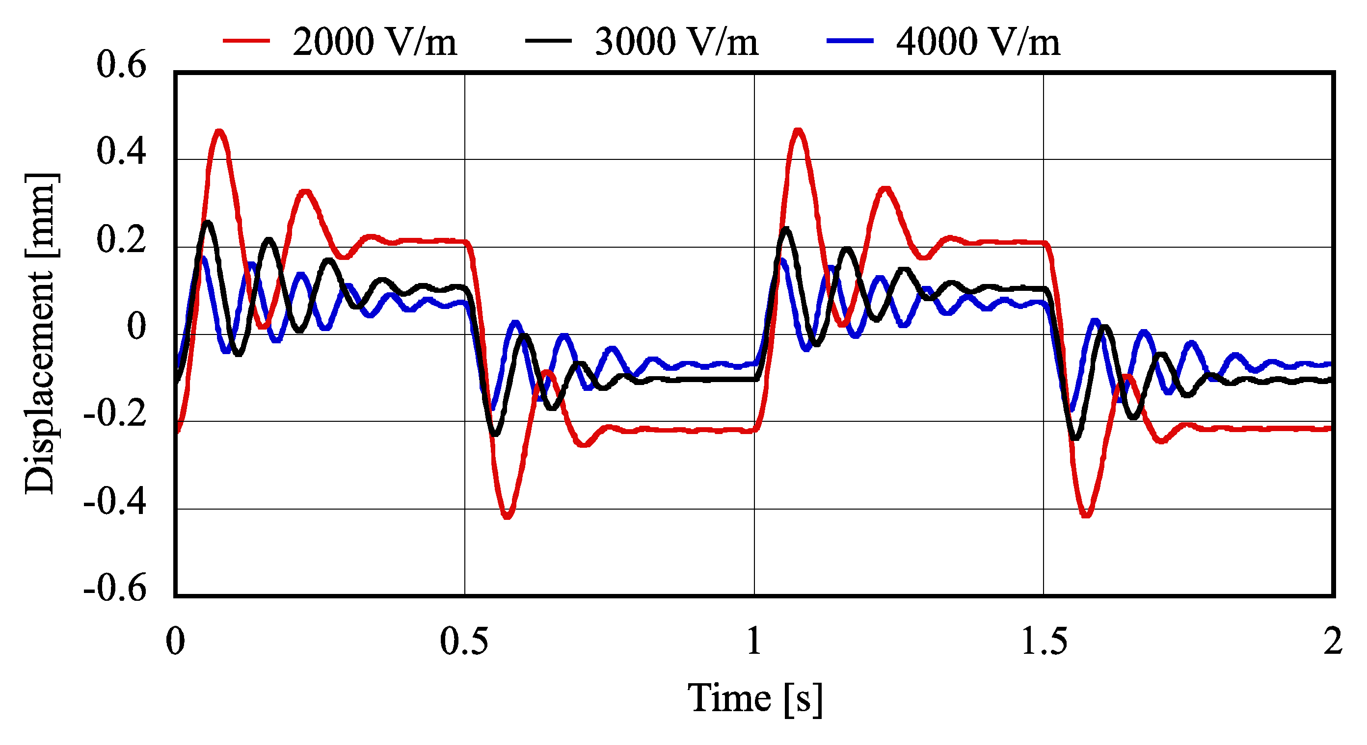
4.1. Responses to Rectangular Disturbance

The responses to a rectangular disturbance are shown in this subsection. The applied rectangular disturbance had a frequency of 1 Hz and an equivalent amplitude of ±0.5 N. A rising of the disturbance occurred at the time of 0. Figure 9 shows the responses when the feedback gain pf was 2000, 3000, and 4000 V/m. When the feedback gain increased, the steady-state displacement tended to be small, the overshoot became large, and the period of the residual vibration became short. These characteristics were similar to those of the PD-controlled system with a higher proportional gain.
Figure 10 shows the responses when the cutoff angular frequency α was 2000, 500, and 200 rad/s. The effect of decreasing the cutoff angular frequency was similar to that of decreasing the proportional gain. The gain of the FORE must be higher than a certain value to produce a restoring force. The reset cycle depended mainly on the cutoff angular frequency of the FORE. The system oscillated due to the reset signal when the frequency of the reset cycle was too low. The output of the LPF diverged when the cutoff frequency was set too high in the time-discrete system.
Figure 11 shows a close look at the FORE output and the displacement after the rising of the disturbance. The cutoff angular frequency was set to 500 rad/s. Under these conditions, a reset action did not occur when the floator was leaving quickly from the zero position (e.g., approximately 0.03 to 0.07 s or 0.14 to 0.20 s). The reset actions occurred when the floator was approaching the zero position (e.g., approximately 0.07 to 0.14 s or 0.20 to 0.30 s). The reset actions occurred also in the steady state (after 0.30 s).
Figure 12 shows a close look at the displacement in the steady state when a static disturbance was applied. The cutoff angular frequency was set to 500 rad/s. The static disturbance was 0.5 N. The other conditions were same as in the previous simulation. The zero in the vertical axis represents the average displacement. A high-frequency vibration and a low-frequency fluctuation were observed in the displacement. The high-frequency vibration occurred due to the reset actions of the FORE. The frequency of the vibration depended on the cutoff angular frequency. The lower frequency fluctuation seemed to be an indeterminate noise. However, no noise applied in the simulation. This fluctuation may have been induced by the operation of the FORE. Therefore, it may have been a unique characteristic of the FORE-controlled system.

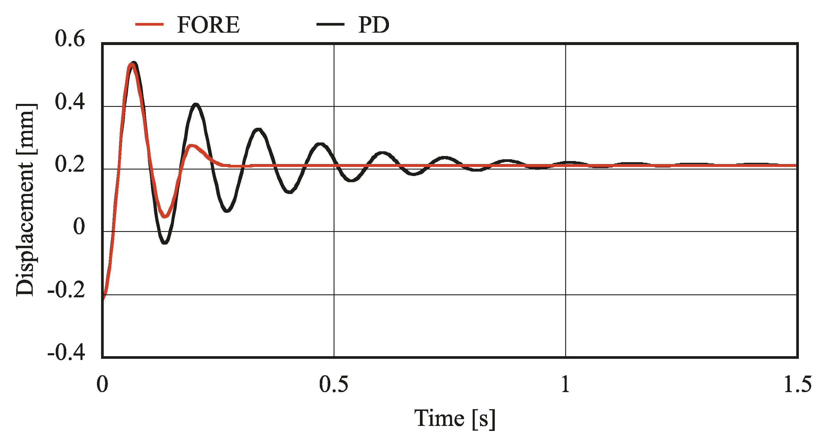
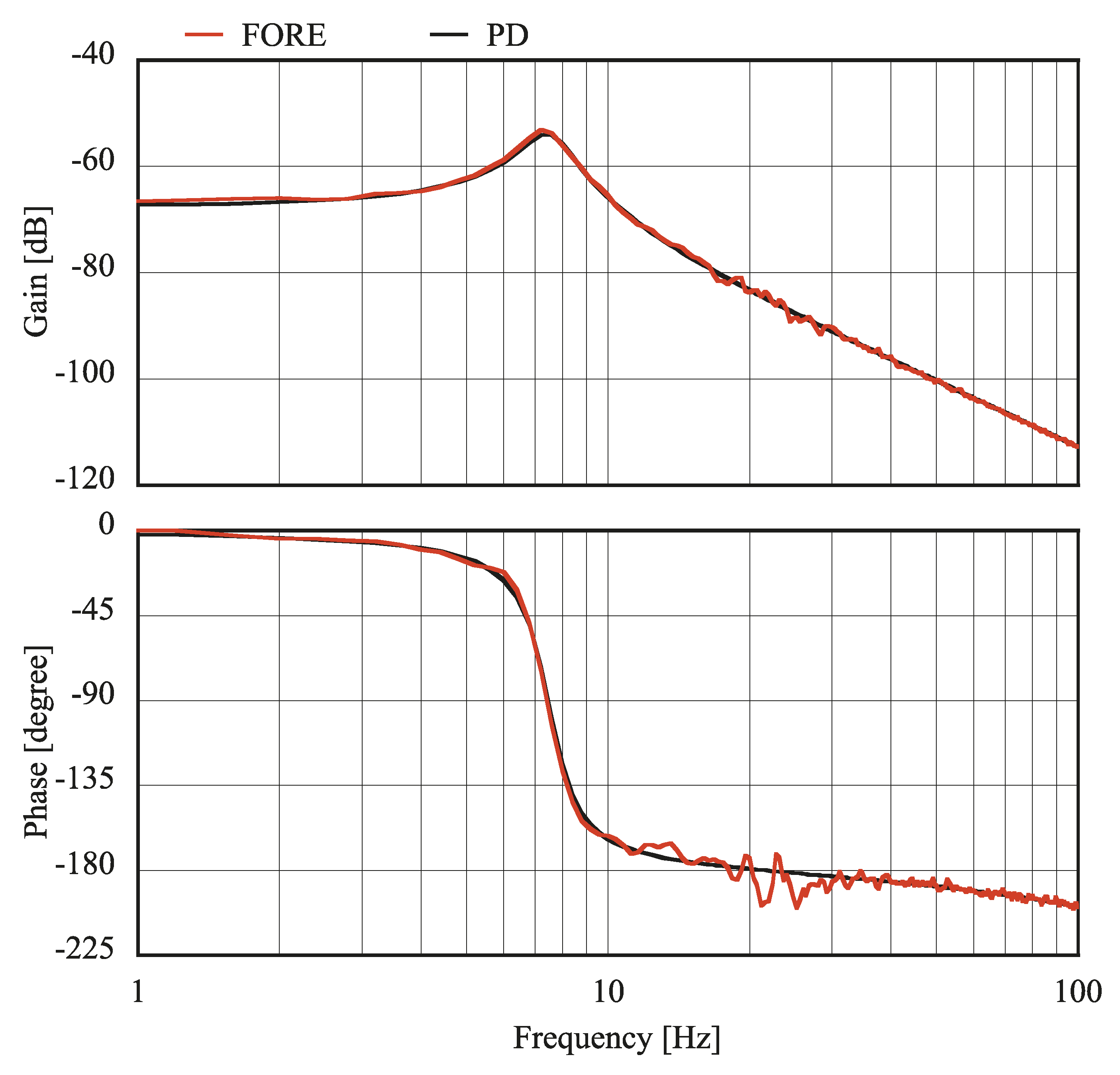
4.2. Comparison of the FORE and PD Control

Figure 13 shows a comparison in time history between the FORE-controlled and PD-controlled systems. The applied disturbance signal had a frequency of 0.5 Hz. The PD controller was designed to have the same first overshoot and the same steady-state displacement as in the step response of the FORE-controlled system. The PD controller had a first-order LPF. The cutoff angular frequency of the LPF (αPD) was the same as that of the FORE for comparison. The transfer function of the PD controller is given by
C P D ( s ) = ( p d + s p v ) α P D s + α P D ,
where pd is the proportional feedback gain and pv is the derivative feedback gain.
The feedback gains and the cutoff angular frequency of the PD controller are
p d = 1720   V / m , p v = 3.8   Vs / m , α P D = 2000   rad / s .
In the FORE-controlled system, the second and subsequent overshoots were reduced more than in the PD-controlled system.
Figure 14 shows a comparison of the frequency response of the displacement-to-disturbance between the FORE- and the PD-controlled systems. The gains of the controllers were the same as in the previous simulation shown by Figure 13. The responses were calculated using an M-sequence with 10 s/cycle and 15 bits. The amount of data in the obtained response was reduced to be one-quarter by averaging every four points.
Even though the step responses were different, the frequency characteristics were similar except for noise-like fluctuations observed in the FORE-controlled system. Such a phenomenon often occurs when an M-sequence is applied to a nonlinear system to obtain frequency responses [15]. These results indicated that there was a possibility that the describing function method may have been ineffective in analyzing the modified FORE-installed system. The noise-like fluctuation was caused by harmonic distortions due to the nonlinearity of the FORE. The harmonic distortions will be discussed in the next subsection.

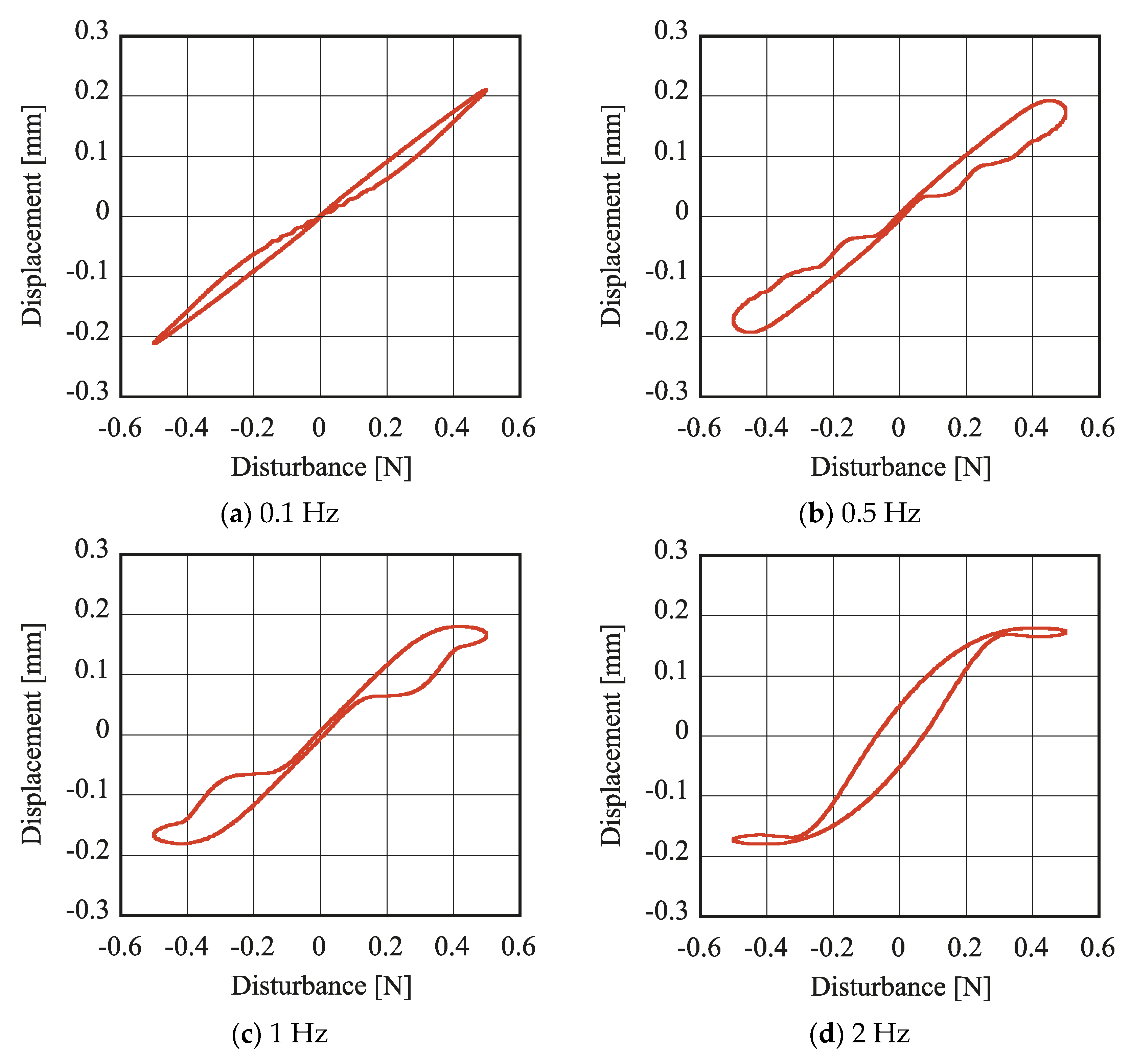
4.3. Lissajous Figures at Various Frequencies

The FORE-controlled system uses a nonlinear element. Therefore, the system may have a noncontinuous response even to a continuous input. Here, the responses to a sinusoidal disturbance were studied. Figure 15 shows the Lissajous figures of the displacement and the disturbance when the frequency of disturbance was varied.
Nonlinear characteristics became noticeable when the floator was displaced from the zero position, especially around 0 N in Figure 15a,b. The effect of the harmonic distortion increased when the frequency became higher, as shown by Figure 15c,d.

5. Experimental Results

This section shows several results of the experiment conducted in the experimental setup shown in Section 3. The conditions of the controller were the same as those described in Section 4.

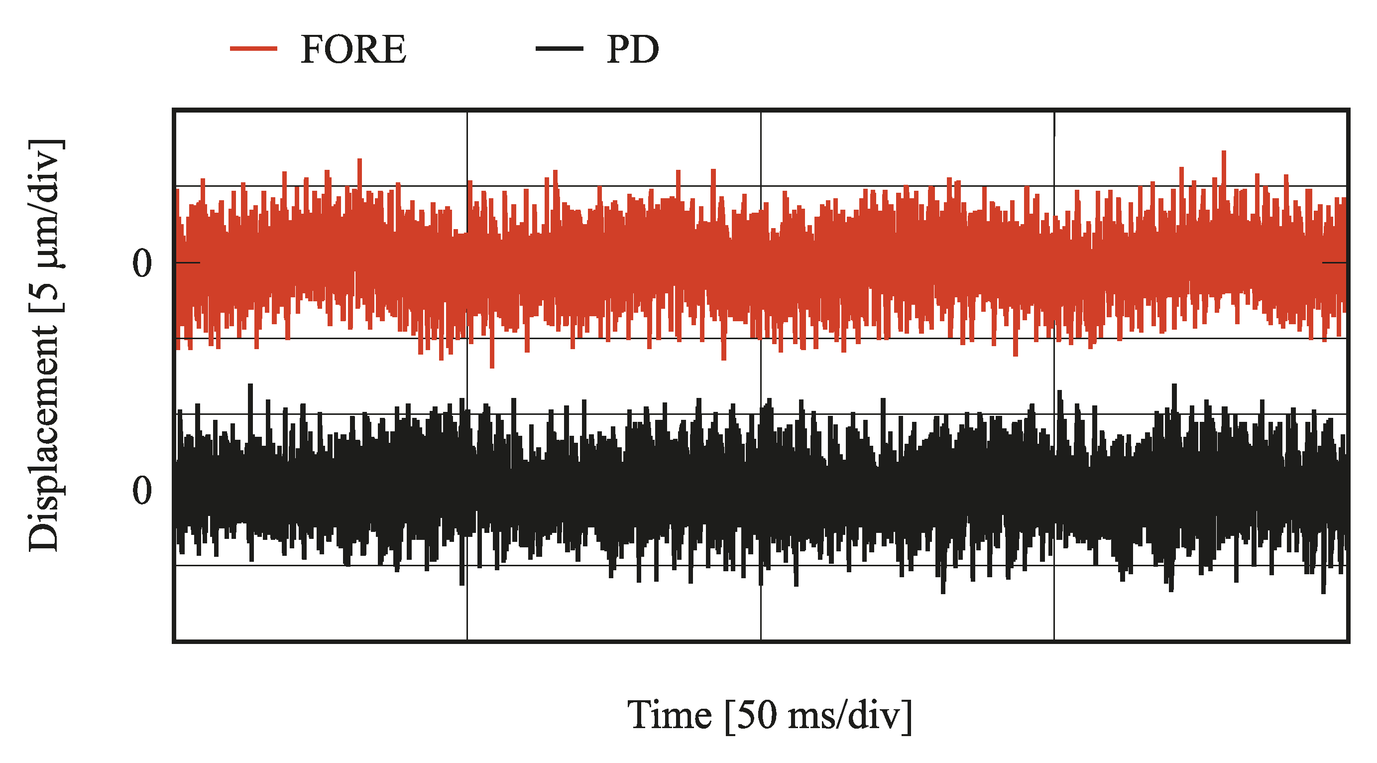
5.1. Confirmation of Stable Suspension

Figure 16 shows a comparison in time history between the FORE- and PD-controlled systems in the steady state. The disturbance was zero. The FORE controller was designed as pf = 2000 V/m and α = 2000 rad/s. The PD controller was designed as described by Equations (7) and (8). A linear integrator with a small gain was inserted parallel to the FORE or PD controller, as mentioned in Section 3.2.
The fluctuations in the steady-state suspension were almost the same in both suspension systems. The fluctuation and the vibration were due to the reset actions shown by Figure 12, and were expected to be smaller than the resolution of the sensor (5 μm). Therefore, such a fluctuation and vibration were not visible in the experiment.

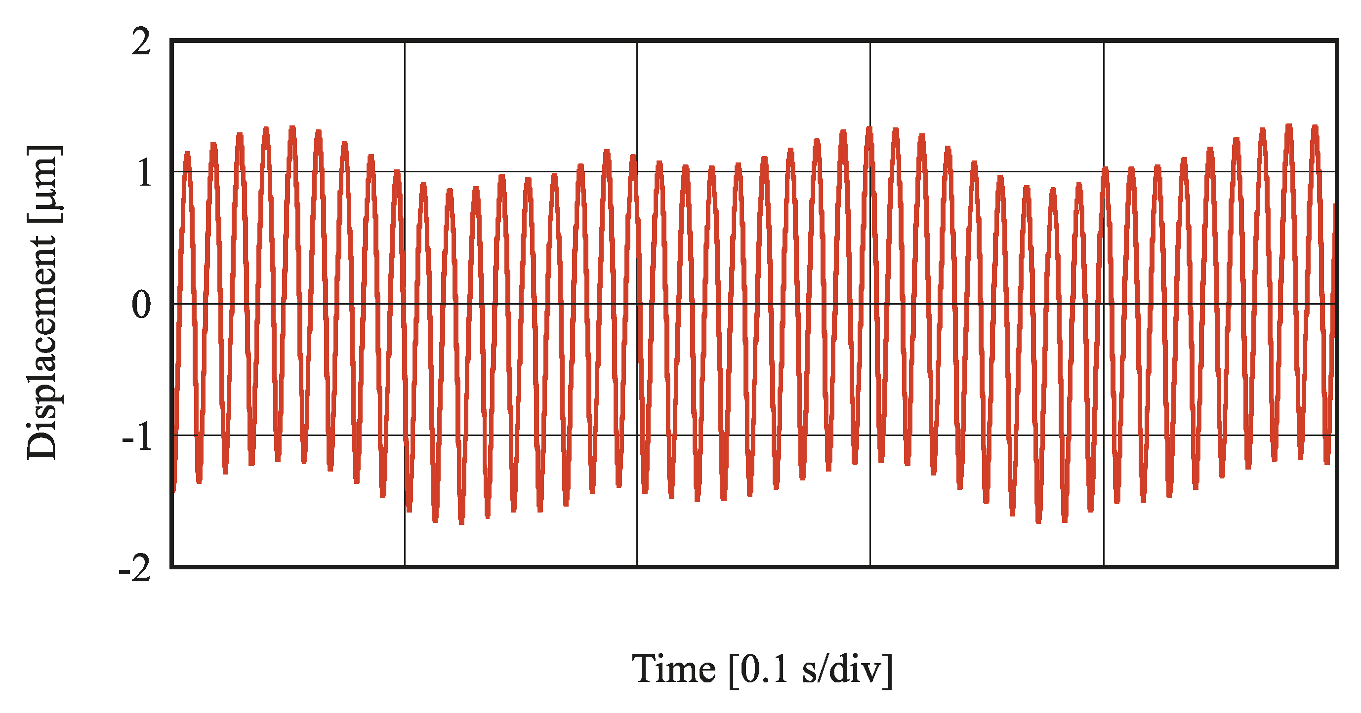
5.2. Responses to Rectangular Disturbance

This subsection shows the responses to a rectangular disturbance. Figure 17 shows the responses when the feedback gain pf was 2000, 3000, or 4000 V/m. Figure 18 shows the responses when the cutoff angular frequency α was 2000, 500, or 200 rad/s. The effects of increasing gain in pf or α were almost the same as in the simulation results shown in Section 4. However, the actual responses were more oscillatory than the simulations. The steady-state position varied depending on the cutoff angular frequency in the simulations, while the position was almost constant in the experiment. The coefficient of the back-electromotive force (kb), the coefficient of the force by the current (ki), and the negative restoring force acting on the hybrid magnet (ks) depended on the gap in the actual system. In the simulation, these coefficients were kept constant. This may have been the reason why the experiment and the simulation results were different.

6. Conclusions

A FORE was introduced as a feedback controller for magnetic suspension. The FORE is a nonlinear LPF using CI. The original FORE was modified to stabilize the magnetic suspension system. The modified FORE achieved the stabilization of a magnetic suspension system without a derivative element. In the stabilized system, a restoring force was produced, and the vibration was damped. The simulation model was a third-order unstable system. The effects of the gain and the cutoff angular frequency on a characteristic closed loop were studied. The stiffness of the system increased when the gain of the FORE became large. The vibration increased by reset actions when the cutoff angular frequency was too low. In the simulation, a small vibration and fluctuations occurred even in the steady state. However, they were not visible in the experiment because the vibration and fluctuations were smaller than the noise included in the displacement signal.

Author Contributions

Conceptualization, Y.I. and T.M.; methodology, Y.I. and M.T.; hardware, Y.I.; formal analysis, Y.I. and M.T.; project administration, T.M.; software, Y.I. and D.Y.; writing—draft, Y.I.; writing—review and editing, T.M., M.T., and D.Y.

Funding

This research received no external funding.

Conflicts of Interest

The authors declare no conflicts of interest.

Nomenclature

SymbolDescriptionUnit
CTransfer function of controllerV/m
CPDTransfer function of PD-controllerV/m
eInput signal of FOREm
FAttractive force between electromagnet and floatorN
gAcceleration due to gravitym/s2
IrCurrent commandV
IeCoil current with equivalent current produced by permanent magnetA
iCurrent of electromagnetA
kaGain of amplifierV/V
kbCoefficient of back electromotive forceVs/m
kiCoefficient of force to currentN/A
ksCoefficient of negative stiffness by hybrid magnetN/m
kxGain of sensorV/m
LInductance of electromagnetH
mMass of floatorkg
mbEquivalent mass of counter balancerkg
pGain of integral feedback used only in the experimentV/ms
pcGain of current sensorV/A
pdGain of proportional feedbackV/m
pfGain of FOREV/m
pvGain of derivative feedbackVs/m
RResistance of electromagnetΩ
tsSampling period of controllers
uOutput signal of FOREV
ûOutput signal of CIV
vOutput voltage of amplifierV
wDisturbance forceN
ŵEquivalent disturbance forceN(V)
xDisplacement of floatorm
αCutoff angular frequency of FORE in linear operationrad/s
αPDCutoff angular frequency of PD controllerrad/s

References

  1. Baños, A.; Barreiro, A. Reset Control Systems; Springer: London, UK, 2012. [Google Scholar]
  2. Clegg, J.C. A nonlinear integrator for servomechanism. Trans. AIEE 1958, 77, 41–42. [Google Scholar] [CrossRef]
  3. Baños, A.; Vidal, A. Design of PC+CI reset compensators for second order plants. In Proceedings of the IEEE International Symposium on Industrial Electronics, Vigo, Spain, 4–7 June 2007. [Google Scholar]
  4. Baños, A.; Vidal, A. Design of Reset Control Systems: The PI plus CI Compensator. J. Dyn. Syst. Meas. Control 2012, 134, 051003. [Google Scholar] [CrossRef]
  5. Horowitz, I.; Rosenbaum, P. Nonlinear design for cost of feedback reduction in systems with large parameter uncertainty. Int. J. Control 1975, 21, 977–1001. [Google Scholar] [CrossRef]
  6. Chait, Y.; Hollot, C.V. On Horowitz’s contributions to reset control. Int. J. Robust Nonlinear Control 2002, 12, 335–355. [Google Scholar] [CrossRef]
  7. Zaccarian, L.; Nesic, D.; Nesic, D.; Teel, A.R. First order reset elements and the Clegg integrator revisited. In Proceedings of the 2005 American Control Conference, Portland, OR, USA, 8–10 June 2005; pp. 563–568. [Google Scholar]
  8. Van Loon, S.J.L.M.; Gruntjens, K.G.J.; Heertjes, M.F.; van de Wouw, N.; Heemels, W.P.M.H. Frequency-domain tools for stability analysis of reset control systems. Automatica 2017, 82, 101–108. [Google Scholar] [CrossRef]
  9. Iwaki, M. Reset Control of Combustion Oscillation in Lean Premixed Combustor. In Proceedings of the 18th International Conference on Control, Automation and Systems (ICCAS), Pyeongchang, Korea, 17–20 October 2018; pp. 207–211. [Google Scholar]
  10. Panni, F.S.; Waschl, H.; Alberer, D.; Zaccarian, L. Position Regulation of an EGR Valve Using Reset Control with Adaptive Feedforward. IEEE Trans. Control Syst. Technol. 2014, 22, 2424–2431. [Google Scholar] [CrossRef]
  11. Acho, L. Nonlinear reset integrator control design: Application to the active suspension control of vehicles. In Proceedings of the IASTED International Conference Modelling, Identification and Control (MIC 2014), Innsbruck, Austria, 17–19 February 2014; pp. 226–228. [Google Scholar]
  12. Sato, M.; Muraoka, K. Flight Test Verification of Flight Controller for Quad Tilt Wing Unmanned Aerial Vehicle. In Proceedings of the AIAA Guidance, Navigation, and Control (GNC) Conference, Boston, MA, USA, 19–22 August 2013. [Google Scholar]
  13. Zheng, J.; Guo, Y.; Fu, M.; Wang, Y.; Xie, L. Improved reset control design for a PZT positioning stage. In Proceedings of the 16th IEEE International Conference on Control Applications, Singapore, 1–3 October 2007. [Google Scholar]
  14. Mizuno, T.; Takemori, Y. A transfer-function approach to the analysis and design of zero-power controllers for magnetic suspension systems. Electr. Eng. Jpn. 2002, 141, 67–75. [Google Scholar] [CrossRef]
  15. Liu, X. Analysis of Pneumatic Control Systems with Bond Graph: Development of a Simulation Software for Pneumatics. Ph.D. Thesis, Saitama University, Saitama, Japan, 1993. [Google Scholar]
Figure 1. Block diagram of original first-order reset element (FORE).
Actuators 08 00024 g001
Figure 2. Block diagram of modified FORE, where etss is the unit delay.
Actuators 08 00024 g002
Figure 3. Simulated time history of the input and output signals in both FOREs. Black line: input signal; heavy red line: output signal of original FORE; blue line: output signal of modified FORE.
Actuators 08 00024 g003
Figure 4. Simulated frequency response of both FOREs. The top represents a gain diagram. The bottom represents a phase diagram. Black line: original FORE; red line: modified FORE.
Actuators 08 00024 g004
Figure 5. Photograph of magnetic suspension apparatus and schematic motion of the floator.
Actuators 08 00024 g005
Figure 6. Schematic view of the electromagnet and floator.
Actuators 08 00024 g006
Figure 7. Block diagram of the magnetic suspension apparatus with the amplifier.
Actuators 08 00024 g007
Figure 8. Block diagram of the magnetic suspension control system. The integrator at the bottom was used only in the experiment.
Actuators 08 00024 g008
Figure 9. Time histories of displacement with a rectangular disturbance in the FORE-controlled system. The feedback gain pf was 2000 V/m (red line), 3000 V/m (black line), and 4000 V/m (blue line).
Actuators 08 00024 g009
Figure 10. Time histories of displacement with a rectangular disturbance in the FORE-controlled system. The cutoff angular frequency was 2000 rad/s (red line), the same as the response in Figure 7, 500 rad/s (black line), and 200 rad/s (blue line).
Actuators 08 00024 g010
Figure 11. Time histories after the rising of disturbance. The top represents the displacement of the floator, and the bottom represents the FORE output.
Actuators 08 00024 g011
Figure 12. A close look at the displacement around the steady-state position.
Actuators 08 00024 g012
Figure 13. Comparison in time history between FORE- and proportional-derivative (PD)-controlled systems. FORE: red line; PD: black line.
Actuators 08 00024 g013
Figure 14. Comparison in frequency response between the FORE- and PD-controlled systems. The top represents the gain diagram. The bottom represents the phase diagram. FORE: red line; PD: black line.
Actuators 08 00024 g014
Figure 15. Lissajous figures of displacement and sinusoidal disturbance.
Actuators 08 00024 g015
Figure 16. Comparison in time history in the steady state. FORE-controlled: blue line; PD-controlled: black line.
Actuators 08 00024 g016
Figure 17. Time histories of displacement to rectangular disturbance in the FORE-controlled system when the feedback gain pf was 2000 V/m (red line), 3000 V/m (black line), and 4000 V/m (blue line).
Actuators 08 00024 g017
Figure 18. Time histories of displacement to rectangular disturbance in the FORE-controlled system when the cutoff angular frequency α was 2000 rad/s (red line), the same as the response in Figure 17, 500 rad/s (black line), and 200 rad/s (blue line).
Actuators 08 00024 g018

