A Physical-State Feedforward Observer with Disturbance-Adaptive Constraint Control for Active Suspension Electro-Hydraulic Actuators

Abstract

The high-performance control of active suspension electro-hydraulic actuators (ASEHA) is limited by a timing mismatch: the primary internal physical state (load pressure) responds to disturbances almost instantaneously, whereas the tracking error used for feedback lags behind. To address this issue, a physics-aware co-design framework introduces three innovations: (i) a pressure-adaptive bandwidth ESO that directly schedules the observer bandwidth via load pressure, enabling faster disturbance estimation; (ii) a disturbance-adaptive constraint controller whose safety boundary is adjusted in real time using the observer‘s disturbance estimates, balancing tracking precision and safety; and (iii) a structured disturbance-separation architecture that reduces observer burden via model-based feedforward. By leveraging load pressure as a feedforward signal, this framework overcomes the latency inherent in error-feedback methods. Comparative simulations show that the proposed method outperforms conventional error-feedback methods by achieving a significant reduction in estimation error, as well as 2.3-times faster convergence, while ensuring both high tracking accuracy and strict constraint satisfaction.

1. Introduction

The active suspension electro-hydraulic actuator (ASEHA) is pivotal for advanced vehicles, as its high-precision control governs ride comfort and handling stability [1]. This demands a control system capable of precise motion tracking despite severe and uncertain disturbances [2,3].

A common approach to addressing this challenge is disturbance estimation using Extended State Observers (ESOs) [4]. Their performance critically depends on observer bandwidth, prompting various adaptive designs where bandwidth is tuned based on feedback from the tracking error [5,6,7,8,9,10]. However, these error-feedback designs inherently suffer from a timing issue: within the ASEHA, a disturbance first perturbs the internal force balance, manifesting almost instantaneously as a change in the load pressure $P_L(t)$—the earliest internal physical-state indicator of force disturbance [11,12]. This pressure change must then drive the mechanical inertia, be measured, and be compared to finally generate the tracking error ${\xi }_1(t)$. Consequently, a conventional error-feedback observer reacts to the system’s past state rather than the immediate physical change.

To address this timing issue, we propose a proactive approach: replacing reactive error-feedback with physical-state feedforward. This shift is realized by the pressure-adaptive bandwidth ESO (PABESO), which couples its bandwidth scheduling directly to the load pressure $P_L(t)$, thereby reducing reliance on the delayed error-feedback loop. This enables faster disturbance estimation and mitigates the phase lag that has long constrained observer-based control.

The timely, high-fidelity disturbance estimates provided by the PABESO enable the downstream controller to tackle a concomitant challenge: enforcing strict safety constraints without conservative performance loss. The Barrier Lyapunov Function (BLF) [13,14,15] is an established mechanism for this. However, conventional BLFs employ static or predefined time-varying boundaries [16,17]. This divorces the safety boundary from available real-time disturbance estimates, leading to a fixed and often conservative trade-off between robustness and precision.

To realize a complete physics-aware co-design framework, we introduce a disturbance-adaptive constraint controller. Its core innovation is a disturbance-adaptive safety boundary $k(t)$ that is directly determined in real-time by the PABESO’s disturbance estimate. This enables a disturbance-aware, feedforward-like coordination, where the boundary relaxes preemptively under large disturbances to preserve feasibility and tightens opportunistically in calm conditions to reclaim performance. Implemented within a compensated command-filtered backstepping framework [18,19,20,21,22], the strategy dynamically resolves the performance–safety trade-off. Thus, the co-design creates a beneficial loop between physical-state perception and constraint-aware action, integrating the components into a unified framework.

Building on this foundation, the disturbance-estimation architecture itself must be refined to further enhance the precision and synergy of the physics-aware co-design framework. This is particularly critical for the ASEHA, where disturbances are heterogeneous, comprising physically modellable components (e.g., viscous friction) and genuinely unknown dynamics [23,24]. While advanced strategies exist, ranging from feedforward cancelation [25] and spectral decomposition [26] to multi-observer architectures [27], they often treat known dynamics as an isolated, static component. This limits the integration of prior physical knowledge into the observer’s core adaptation loop. Consequently, the observer remains burdened, limiting the overall framework’s estimation accuracy and robustness.

To overcome this limitation and realize a physics-aware co-design, we introduce a structured disturbance-separation architecture as the third component. It explicitly decomposes disturbances into a physically modellable part $d_{phy}(t)$ for feedforward cancelation and a genuinely unknown residual $d_{ext}(t)$ for the PABESO’s focused estimation. By offloading the observer with this prior physical knowledge, the architecture allows the PABESO to focus more on truly uncertain dynamics. The resulting estimates provide improved support for the disturbance-adaptive constraint management, thereby contributing to an integrated three-component co-design.

Thus, the proposed physics-aware co-design framework integrates three synergistic components: a physical-state feedforward observer, a disturbance-adaptive constraint controller, and a structured disturbance-separation architecture. Together, they form a co-design framework that combines disturbance observation and constraint-aware control. The main contributions of this work are therefore threefold:

(1)

A physical-state feedforward observer (PABESO) that uses load-pressure as a feedforward signal for bandwidth tuning, enabling faster disturbance estimation.

(2)

A disturbance-adaptive constraint controller that leverages the PABESO’s disturbance estimates to dynamically adjust the safety boundary, enabling an adaptive performance–safety trade-off.

(3)

A structured disturbance-separation architecture that actively embeds prior physical knowledge to offload the observer, thereby improving estimation accuracy and reducing observer burden.

The remainder of this paper is organized as follows. Section 2 presents the nonlinear dynamic model of the ASEHA. Section 3 details the physics-aware co-design framework, introducing the physical-state feedforward observer in Section 3.1 and the disturbance-adaptive constraint controller in Section 3.2. Rigorous stability analysis of the proposed observer and the closed-loop system is provided in Section 4. Comparative simulations and discussions are presented in Section 5. Finally, Section 6 concludes the paper.

2. Nonlinear Dynamic Model of the ASEHA

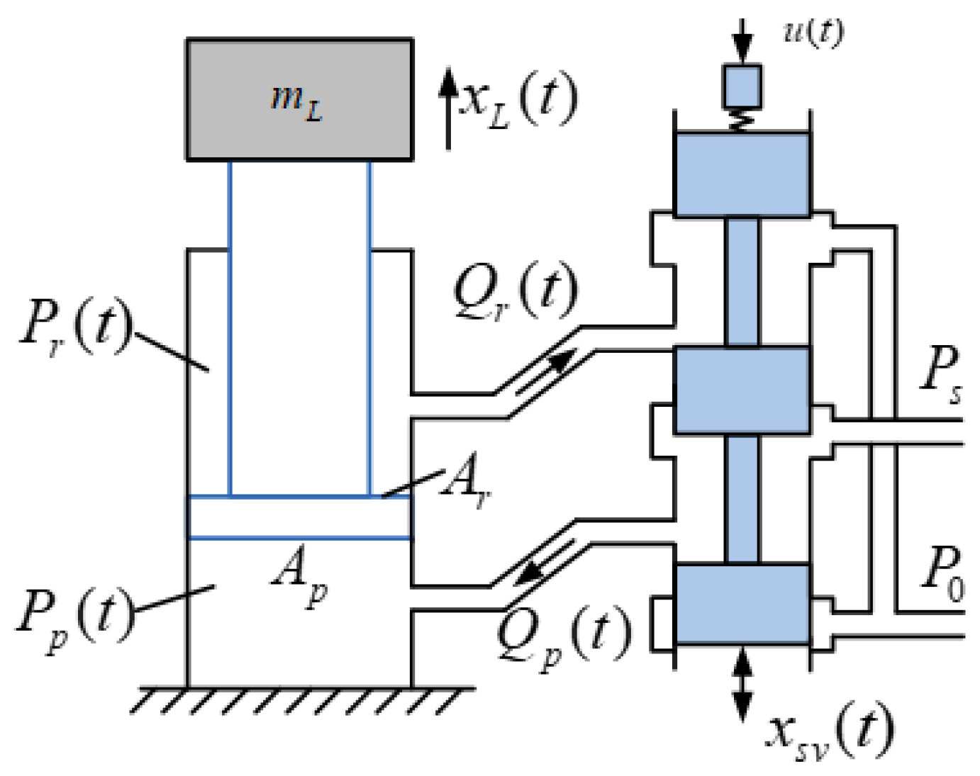
The configuration of a single suspension unit is illustrated in Figure 1. The model incorporates the following key variables: the effective piston areas of the cap and rod sides, denoted by $A_p$ and $A_r$, respectively; the corresponding chamber pressures $P_p(t)$ and $P_r(t)$; the hydraulic flow rates $Q_p(t)$ (inflow) and $Q_r(t)$ (outflow); the system supply and return pressures $P_s$ and $P_0$; the sprung mass $m_L$ and its vertical displacement $x_L(t)$; the servo valve spool displacement $x_{sv}(t)$; and the servo valve control current $u(t)$.

The motion dynamics of the sprung mass follow Newton’s second law [1]

$$m_L{\ddot{x}}_L(t)=F_{hyd}(t)-m_{L}g-B{\dot{x}}_L(t)-F_f(t)$$

(1)

where g is the gravitational acceleration, $B$ denotes the viscous damping coefficient of the hydraulic fluid, and $F_f(t)$ represents the lumped mechanical disturbance that includes unmodeled friction and other external disturbances. The term $F_{hyd}(t)=P_p(t)A_p-P_r(t)A_r$ is the net hydraulic driving force.

Remark 1

(Load pressure as an early disturbance indicator). From the force balance Equation (1), the net hydraulic driving force is

$$F_{hyd}(t)=P_p(t)A_p-P_r(t)A_r$$

Following the standard definition in hydraulic systems [28], the load pressure is defined as

$$P_L(t)=P_p(t)-P_r(t)(A_r/A_p)$$

Substituting this definition into  $F_{hyd}(t)$ yields

$$F_{hyd}(t)=A_p{P}_L(t)$$

Hence, $P_L(t)$ is algebraically proportional to the net hydraulic force and changes instantaneously when a disturbance alters the force balance.

In hydraulic systems, pressure dynamics respond significantly faster than mechanical displacements due to the high bulk modulus of the fluid (typically ${10}^8-{10}^9\mathrm{Pa}$) [12,29]. When a disturbance occurs, it first perturbs the force balance, which manifests immediately as a change in $P_L(t)$. This pressure change then propagates through the mechanical inertia—requiring integration from acceleration to velocity to displacement—before appearing in the tracking error ${\xi }_1(t)=x_L(t)-x_d(t)$. Consequently, $P_L(t)$ provides a leading-phase signal compared to the displacement-based feedback error.

Based on the load-flow continuity equation, the pressure dynamics in the two chambers of the hydraulic cylinder are given by the following nonlinear differential equations:

$${\dot{P}}_p(t)={\displaystyle \frac{{\beta }_e}{V_p(t)}}[-A_p{\dot{x}}_L(t)-c_{ip}(P_p(t)-P_r(t))+Q_p(t)+w_p(t)]$$

(2)

$${\dot{P}}_r(t)={\displaystyle \frac{{\beta }_e}{V_r(t)}}[A_l{\dot{x}}_L(t)+c_{ip}(P_p(t)-P_r(t))-c_{ep}{P}_r(t)-Q_r(t)+w_r(t)]$$

(3)

where ${\beta }_e$ is the effective bulk modulus of the hydraulic fluid; $c_{ip}$ and $c_{ep}$ are the internal and external leakage coefficients of the cylinder, respectively; $w_p(t)$ and $w_r(t)$ represent system disturbances; and $V_p(t)=V_{p0}+A_p{x}_L(t)$ and $V_r(t)=V_{r0}+A_r{x}_L(t)$ denote the instantaneous volumes of the cap and rod sides, with $V_{p0}$ and $V_{r0}$ being their initial volumes.

The flow rates $Q_p(t)$ and $Q_r(t)$ are proportional to the spool displacement and exhibit a nonlinear relationship with the pressure difference [25], modeled as follows:

$$Q_p(t)=k_t{x}_{sv}(t){\mathsf{\Psi }}_1$$

(4)

$$Q_r(t)=k_t{x}_{sv}(t){\mathsf{\Psi }}_2$$

(5)

where $k_t=C_d\omega \sqrt{2/\rho }$ is the flow-rate coefficient, with $C_d$ being the discharge coefficient; $\omega$ is the spool area gradient; and $\rho$ is the fluid density. The terms ${\mathsf{\Psi }}_1$ and ${\mathsf{\Psi }}_2$ represent the direction-dependent pressure-flow nonlinearities, defined as ${\mathsf{\Psi }}_1=H(u(t))\sqrt{P_s-P_p(t)}$ $+H(-u(t))$ $\sqrt{P_p(t)-P_0}$, ${\mathsf{\Psi }}_2=H(u(t))\sqrt{P_r(t)-P_0}+H(u(t))\sqrt{P_s-P_r(t)}$, with $H(·)$ being the Heaviside step function. Given that the spool response is significantly faster than the actuator dynamics, the spool displacement is assumed to be proportional to the control current, i.e., $x_{sv}(t)=k_{sv}u(t)$, where $k_{sv}$ is the proportional gain.

To address the inherent nonlinearities and parametric uncertainties of the hydraulic system, the following assumption is introduced:

Assumption 1.

The disturbances  $w_p(t)$ and $w_r(t)$ are continuously differentiable, and modeling errors arising from variations in ${\beta }_e$, $c_{ip}$, and $c_{ep}$ are incorporated into $w_p(t)$ and $w_r(t)$.

Under Assumption 1, the state vector is defined as $X(t)={[x_1(t),x_2(t),x_3(t)]}^T$ $={[x_L(t),{\dot{x}}_L(t),{\ddot{\mathrm{x}}}_L(t)]}^T$, and the system’s output is $y(t)=x_1(t)$. The ASEHA dynamics (1)–(5) can be expressed in the following state-space form [30], which explicitly highlights the nonlinear control-affine structure and the lumped disturbance term:

$$\left\{\begin{array}{l}{\dot{x}}_1(t)=x_2(t)\hfill \\ {\dot{x}}_2(t)=x_3(t)\hfill \\ {\dot{x}}_3(t)={\alpha }_h{x}_2(t)+{\beta }_h{x}_3(t)+{\gamma }_{u}u(t)+d(t)\hfill \end{array}\right.$$

(6)

In (6), the coefficients and disturbance term are defined as follows:

$$\begin{array}{l}{\alpha }_h=-{\displaystyle \frac{{\beta }_e}{m_L}}\left({\displaystyle \frac{A_{\mathrm{p}}^2}{V_p(t)}}+{\displaystyle \frac{A_r^2}{V_r(t)}}\right)-{\displaystyle \frac{2{\beta }_e{C}_{ip}{b}_s}{m_L(A_p+A_r)}}\left({\displaystyle \frac{A_p}{V_p(t)}}+{\displaystyle \frac{A_r}{V_r(t)}}\right),\\ {\beta }_h=-{\displaystyle \frac{b_s}{m_L}}-{\displaystyle \frac{2{\beta }_e{C}_{ip}}{A_p+A_r}}\left({\displaystyle \frac{A_p}{V_p(t)}}+{\displaystyle \frac{A_r}{V_r(t)}}\right),\\ {\gamma }_u={\displaystyle \frac{{\beta }_e}{m_L}}{k}_q{k}_i\left({\displaystyle \frac{A_p}{V_r(t)}}{\mathsf{\Psi }}_1+{\displaystyle \frac{A_p}{V_r(t)}}{\mathsf{\Psi }}_2\right),\\ d(t)=d_{phy}(t)+d_{ext,}(t)\end{array},$$

Physically, ${\alpha }_h$ reflects the combined hydraulic stiffness and leakage-induced damping, ${\beta }_h$ governs the energy dissipation due to viscous friction, and ${\gamma }_u$ is the control input gain determined by the pressure-flow nonlinearities ${\mathsf{\Psi }}_1$ and ${\mathsf{\Psi }}_2$. The lumped disturbance $d(t)$ is decomposed into a physically modellable part $d_{phy}(t)$ and an uncertain residual $d_{ext}(t)$, where $d_{ext}(t)$ contains unknown friction $F_f(t)$, unmeasurable disturbances $w_p(t),w_r(t)$, and any modeling errors in $d_{phy}(t)$.

The physically modellable part $d_{phy}(t)$ is selected as:

$$d_{phy}(t)=-{\displaystyle \frac{2{\beta }_e{c}_{ip}}{A_p+A_r}}\left({\displaystyle \frac{A_p}{V_p(t)}}+{\displaystyle \frac{A_r}{V_r(t)}}\right)g+{\displaystyle \frac{{\beta }_e}{m_L}}{\displaystyle \frac{A_r}{V_r}}{c}_{ep}{P}_r(t),$$

where ${\beta }_e,c_{ip},c_{ep}$ are nominal values (obtainable from offline identification or manufacturer data), and $V_p(t),V_r(t),P_r(t)$ are obtained from displacement and pressure measurements. This separation offloads the observer via feedforward cancellation of $d_{phy}(t)$, allowing it to focus on the uncertain residual $d_{ext}(t)$.

Remark 2

(On force approximation). The approximation $(P_p(t)-P_r(t))(A_p+A_r)\approx 2(P_p(t)$ $A_p-P_r(t)A_r)$ is made for analytical tractability, with its error absorbed into the system disturbances.

Assumption 2.

The term  $d_{ext}(t)$ encompasses all unmodeled dynamics, and its first-time derivative is bounded, i.e., there exists a positive constant $\overline{d}$ such that $|{\dot{d}}_{ext}(t)|\le \overline{d}$ for all $t\ge 0$.

Assumption 3.

The desired displacement trajectory $x_d(t)$ is continuously differentiable up to the third order, and its derivatives are bounded. Specifically, there exist positive constants ${\overline{x}}_d$, ${\overline{v}}_d$ and ${\overline{a}}_d$ such that $\left|x_d\right|\le {\overline{x}}_d$, $\left|{\dot{x}}_d\right|\le {\overline{v}}_d$, and $\left|{\ddot{x}}_d\right|\le {\overline{a}}_d$ for all $t\ge 0$.

3. The Physics-Aware Co-Design Framework

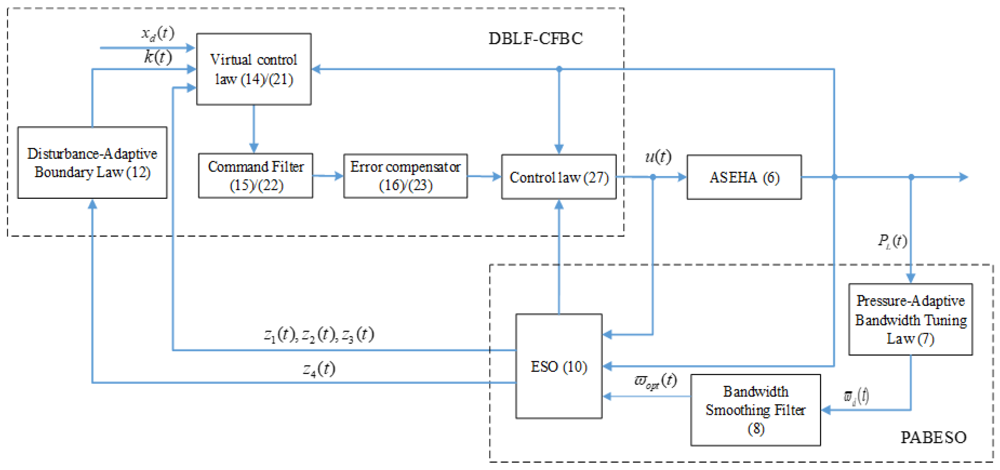
This section presents a co-designed framework. Different from conventional error-feedback-based observers and static-boundary BLF controllers, the framework introduces two interlocking innovations (Figure 2): (i) the pressure-adaptive bandwidth ESO (PABESO), which implements the physical-state feedforward principle by using the load pressure to directly schedule observer bandwidth; and (ii) disturbance-adaptive constraint enforcement via a disturbance-adaptive boundary law $k(t)$, where the feasible region expands/contracts with the real-time disturbance estimate $z_4(t)$. The following subsections detail their design.

3.1. Design of the Physical-State Feedforward Observer (PABESO)

Unlike conventional error-feedback-based observers, the proposed PABESO implements the physical-state feedforward principle. Its design is motivated by the causal primacy of the load pressure $P_L(t)$, which provides the earliest indicator of disturbances.

The PABESO is constructed to estimate the state vector $z_1(t),z_2(t),z_3(t)$ along with the unknown disturbance $d_{ext}(t)$. Defining the estimation vector as $\mathit{z}(t)={[z_1(t),z_2(t),z_3(t),z_4(t)]}^T$. The pressure-adaptive bandwidth tuning law ${\varpi }_d(t)$ employs a hyperbolic tangent function for pressure-dependent adjustment:

$${\varpi }_d(t)=\left\{\begin{array}{cc}{\omega }_{\min },\hfill & \left|P_L(t)-P_{nom}\right|<{\delta }_P\hfill \\ {\omega }_{\min }+({\omega }_{\max }-{\omega }_{\min })\cdot \tanh (\eta {\displaystyle \frac{\left|P_L(t)-P_{nom}\right|-{\delta }_P}{P_{max}}}),\hfill & otherwise\hfill \end{array}\right.$$

(7)

In the above expression, $P_L(t)$ denotes the load pressure, $P_{nom}$ its nominal value, and ${\delta }_P$ is the pressure deviation threshold. The parameters ${\omega }_{\min }$ and ${\omega }_{\max }$ define the minimum and maximum bandwidth limits, respectively; $\eta$ is a tuning gain controlling the sensitivity of bandwidth to pressure variations; and $P_{\max }$ serves as a normalization factor to constrain the input range.

Remark 3

(Features of the bandwidth tuning law). The tuning law (7) implements the physical-state feedforward principle through three key features: (i) Pressure-driven adaptation: The bandwidth adjusts proactively with the load pressure deviation $\left|P_L(t)-P_{nom}\right|$, reducing the latency inherent in error-based adaptation. (ii) Smooth trade-off: The $\tanh (·)$ transition, governed by $\eta$, balances the competing requirements of fast disturbance response and steady-state noise rejection. (iii) Implementation robustness: The deadzone ${\delta }_P$ provides built-in robustness to measurement noise, while the continuous function avoids chattering and excitation of unmodeled dynamics.

In practice, this pressure-driven bandwidth scheduling enables the controller to respond to road disturbances (e.g., speed bumps) almost instantaneously, reducing the time delay that causes passenger discomfort in conventional systems.

To prevent abrupt transitions in bandwidth due to transient fluctuations or measurement noise in the load pressure $P_L(t)$, a bandwidth smoothing filter [31] is introduced to smooth the desired bandwidth:

$${\dot{\varpi }}_{opt}(t)=-{\tau }^{-1}{\varpi }_{opt}(t)+{\tau }^{-1}{\varpi }_d(t)+K_f{\dot{\varpi }}_d(t)$$

(8)

where $\tau$ is the time constant and $0<K_f<1$ is the derivative feedforward gain.

The time-varying gain matrix $\mathit{K}({\varpi }_{opt}(t))$ is designed via the bandwidth parameterization approach:

$$\mathit{K}({\varpi }_{opt}(t))={[l_1{\varpi }_{opt}(t),l_2{\varpi }_{opt}^2(t),l_3{\varpi }_{opt}^3(t),l_4{\varpi }_{opt}^4(t)]}^T$$

(9)

Here, $l_i$ are observer gain coefficients.

Finally, the observer dynamics are given by:

$$\dot{\mathbf{z}}(t)={\mathit{A}}_h\mathbf{z}(t)+{\mathit{B}}_{u}u(t)+\mathit{F}{d}_{phy}(t)+\mathit{K}({\varpi }_{opt}(t))e(t)$$

(10)

where $e(t)=y(t)-z_1(t)$ is the output estimation error and the system matrix ${\mathit{A}}_h$ is structured as:

$${\mathit{A}}_h=\left[\begin{array}{cccc}0& 1& 0& 0\\ 0& 0& 1& 0\\ 0& {\alpha }_h& {\beta }_h& 1\\ 0& 0& 0& 0\end{array}\right]$$

The control input matrix ${\mathit{B}}_u={[0,0,{\gamma }_u,0]}^T$ reflects the actuation gain, while the disturbance matrix $\mathit{F}={[0,0,1,0]}^T$ directs the modellable physical disturbance $d_{phy}(t)$ into the corresponding dynamic channel.

3.2. Design of the Disturbance-Adaptive Constraint Controller (DBLF-CFBC)

This subsection details the disturbance-adaptive constraint controller, which constructs its disturbance-adaptive boundary from the PABESO’s estimates, directly addressing the latency issue in constraint enforcement. Under Assumption 3, the tracking error is defined as ${\xi }_1(t)=x_1(t)-x_d(t)$, where $x_d(t)$ denotes the desired displacement. To enforce time-varying state constraints, the following DBLF is constructed:

$$V_1={\displaystyle \frac{1}{2}}\tan ({\displaystyle \frac{\pi {\xi }_1^2(t)}{2k^2(t)}})$$

(11)

The key novelty of the proposed controller lies in the disturbance-adaptive boundary:

$$k(t)=k_0{e}^{-{\lambda }_{c}t}+{\mu }_c\left|z_4(t)\right|+k_{\infty }$$

(12)

Here, $k_0>\left|{\xi }_1(0)\right|$ prevents initial input saturation, $k_{\infty }>0$ sets the steady-state accuracy, ${\lambda }_c>0$ governs the transient-to-steady-state decay, and ${\mu }_c>0$ is a disturbance-adaptive gain.

In (12), the component $k_0{e}^{-{\lambda }_{c}t}+k_{\infty }$ forms a prescribed performance funnel, shaping the desired transient and steady-state behavior. Distinct from conventional BLF methods with fixed or pre-defined time-varying boundaries, the proposed novel term ${\mu }_c\left|z_4(t)\right|$, where $z_4(t)$ is the PABESO’s disturbance estimate, provides a feedforward action that actively expands the feasible region under large disturbances, preempting constraint violation and boosting closed-loop robustness. Moreover, (12) directly implies $k(t)\ge k_{\infty }>0$ for all $t\ge 0$, ensuring the boundary is strictly positive and well-defined.

Differentiating $V_1$ with respect to time yields:

$${\dot{V}}_1={\displaystyle \frac{\pi {\xi }_1(t)}{2k^2(t)}}se{c}^2({\displaystyle \frac{\pi {\xi }_1^2(t)}{2k^2(t)}}){\dot{\xi }}_1(t)-{\displaystyle \frac{\pi {\xi }_1^2(t)}{2k^3(t)}}se{c}^2({\displaystyle \frac{\pi {\xi }_1^2(t)}{2k^2(t)}})\dot{k}(t)$$

(13)

In (13), the first term reflects the sensitivity to the tracking error dynamics, and the second term accounts for the adaptation of the time-varying boundary $k(t)$.

The virtual control law is designed as

$${\alpha }_1(t)={\dot{x}}_d-K_1{\xi }_1(t){\displaystyle \frac{2k^2(t)}{\pi }}{\cos }^2({\displaystyle \frac{\pi {\xi }_1^2(t)}{2k^2(t)}})+{\xi }_1(t){\displaystyle \frac{\dot{k}(t)}{k(t)}}$$

(14)

where $K_1>0$ is the controller gain. The term ${\xi }_1(t){\displaystyle \frac{\dot{k}(t)}{k(t)}}$ in the virtual control law (14) is designed to cancel the time-varying boundary effect arising from $\dot{k}(t)$.

To synthesize the smoothed virtual control signal required for constraint-aware stabilization, the following command filter is introduced

$$\left\{\begin{array}{l}{\dot{\chi }}_{1,1}(t)={\chi }_{1,2}(t)\\ {\dot{\chi }}_{1,2}(t)=-2{\varsigma }_1{\omega }_{n1}{\chi }_{1,2}(t)-{\omega }_{n1}^2({\chi }_{1,1}(t)-{\alpha }_1(t))\end{array}\right.$$

(15)

where ${\varsigma }_1>0$ and ${\omega }_{n1}>0$ are the damping ratio and bandwidth of the filter, respectively; ${\chi }_{1,1}(t)={\alpha }_{1f}(t)$ represents the filtered virtual control law, and ${\chi }_{1,2}(t)={\dot{\alpha }}_{1f}(t)$ is its derivative.

Lemma 1

(Boundedness of command filter error [21,32]). Consider the command filter in (15) with initial conditions ${\chi }_{1,1}(0)={\alpha }_1(0)$,  ${\chi }_{1,2}(0)=0$. If the input signal  ${\alpha }_1$ satisfies  $\left|{\dot{\alpha }}_1\right|\le {\overline{\alpha }}_1$ and  $\left|{\ddot{\alpha }}_1\right|\le {\overline{\alpha }}_2$, where  ${\overline{\alpha }}_1,{\overline{\alpha }}_2>0$ are constants, then for any $\mu >0$, there exist filter parameters  ${\varsigma }_1\in (0,1]$, and  ${\omega }_{n1}>0$, such that the output signals  ${\alpha }_{1f}(t)={\chi }_{1,1}(t)$ and  ${\dot{\alpha }}_{1f}(t)={\chi }_{1,2}(t)$ are bounded, and the filtering error satisfies  $|{\alpha }_{1f}(t)-{\alpha }_1(t)|\le \mu$.

Although Lemma 1 ensures that the filtering error can be made arbitrarily small, the following error compensation system is introduced to fully eliminate its influence on stability

$${\dot{\upsilon }}_1(t)=-{\varrho }_1{\upsilon }_1(t)+({\alpha }_{1f}(t)-{\alpha }_1(t)),{\varrho }_1>0$$

(16)

Using the filter output and compensation signal, a new tracking error is defined as

$${\xi }_2(t)=z_2(t)-{\alpha }_{1f}(t)-{\upsilon }_1(t)$$

(17)

Substituting the system dynamics and the above definitions into ${\dot{V}}_1$, we obtain

$${\dot{V}}_1=-K_1{\xi }_1^2(t)+\Xi {\xi }_1(t){\xi }_2(t)+\Xi {\xi }_1(t)[{\alpha }_{1f}(t)-{\alpha }_1(t)+{\upsilon }_1(t)+e_2(t)]$$

(18)

where the nonlinear gain is defined as $\Xi ={\displaystyle \frac{\pi }{2k^2(t)}}se{c}^2({\displaystyle \frac{\pi {\xi }_1^2(t)}{2k^2(t)}})$.

The derivative shows that the derivative of the Lyapunov function consists of three components: a negative definite stabilizing term, an interconnection term with the next-level error ${\xi }_2(t)$, and a coupling term that contains the command filtering error and compensation signal. The error compensation system is designed specifically to suppress this coupling term. To stabilize the entire closed-loop system, the following augmented Lyapunov function is constructed

$$V_2=V_1+{\displaystyle \frac{1}{2}}{\xi }_2^2(t)+{\displaystyle \frac{1}{2}}{\upsilon }_1^2(t)$$

(19)

Combining (10), (16) and (17), the derivative of $V_2$ is derived as

$$\begin{array}{cc}\hfill {\dot{V}}_2& =-K_1{\xi }_1^2(t)-{\varrho }_1{\upsilon }_1^2(t)+\Xi {\xi }_1(t)({\alpha }_{1f}(t)-{\alpha }_1(t)+{\upsilon }_1(t)+e_2(t))+{\upsilon }_1(t)({\alpha }_{1f}(t)-{\alpha }_1(t))\\ & +{\xi }_2(t)[z_3(t)+l_2{\varpi }_{opt}^2{e}_1-{\dot{\alpha }}_{1f}(t)+{\varrho }_1{\upsilon }_1(t)-({\alpha }_{1f}(t)-{\alpha }_1(t))+\Xi {\xi }_1(t)]\hfill \end{array}$$

(20)

Remark 4

(Boundedness of the $\Xi$). Since the time-varying constraint boundary $k(t)$ satisfies  $k_{\min }>0$, the denominator of the nonlinear gain  $\Xi$ has a deterministic upper bound of  $2k_{\min }^2$ . Furthermore, the argument of the  ${\sec }^2(\cdot )$ function,  $\pi {\xi }_1^2(t)/(2k^2(t))$, is strictly confined to the interval  $[0,\pi /2)$, thereby ensuring the boundedness of  ${\sec }^2(\cdot )$ over this domain. Consequently, there exists a positive constant  ${\Xi }_{\max }$ such that  $\Xi (t)\le {\Xi }_{\max }$ hold for all  $t\ge 0$.

To stabilize the error state ${\xi }_2(t)$, the virtual control law is designed as:

$${\alpha }_2(t)={\dot{\alpha }}_{1f}(t)-{\varrho }_1{\upsilon }_1(t)+({\alpha }_{1f}(t)-{\alpha }_1(t))-\Xi {\xi }_1(t)-l_2{\varpi }_{opt}^2{e}_1(t)-K_2{\xi }_2(t)$$

(21)

where $K_2>0$ is a controller gain. The signal ${\alpha }_2(t)$ is then passed through the following command filter to obtain a continuous filtered signal.

$$\left\{\begin{array}{l}{\dot{\chi }}_{2,1}(t)={\chi }_{2,2}(t)\\ {\dot{\chi }}_{2,2}(t)=-2{\varsigma }_2{\omega }_{n2}{\chi }_{2,2}(t)-{\omega }_{n2}^2({\chi }_{2,1}(t)-{\alpha }_2(t))\end{array}\right.$$

(22)

The outputs are defined as the filtered virtual control signal and its derivative: ${\chi }_{2,1}(t)={\alpha }_{2f}(t)$, ${\chi }_{2,2}(t)={\dot{\alpha }}_{2f}(t)$. To suppress the estimation error of the second-stage filter, the following compensation dynamics are introduced:

$${\dot{\upsilon }}_2(t)=-{\varrho }_2{\upsilon }_2(t)+({\alpha }_{2f}(t)-{\alpha }_2(t)),{\varrho }_2>0$$

(23)

Defining ${\xi }_3(t)=z_3(t)-{\alpha }_{2f}(t)-{\upsilon }_2(t)$ and substituting $z_3(t)={\xi }_3(t)+{\alpha }_{2f}(t)+{\upsilon }_2(t)$ together with (21) into ${\dot{V}}_2$, we obtain

$$\begin{array}{cc}\hfill {\dot{V}}_2& =-K_1{\xi }_1^2(t)-{\varrho }_1{\upsilon }_1^2(t)-K_2{\xi }_2^2(t)+{\xi }_2(t){\xi }_3(t)\hfill \\ & +\Xi {\xi }_1(t)({\alpha }_{1f}(t)-{\alpha }_1(t)+{\upsilon }_1(t)+e_2(t))+{\upsilon }_1(t)({\alpha }_{1f}(t)-{\alpha }_1(t))\hfill \\ & +{\xi }_2(t)({\alpha }_{2f}(t)-{\alpha }_2(t))+{\xi }_2(t){\upsilon }_2(t)\hfill \end{array}$$

(24)

A global Lyapunov function is constructed as

$$V_3=V_2+{\displaystyle \frac{1}{2}}{\xi }_3^2(t)+{\displaystyle \frac{1}{2}}{\upsilon }_2^2(t)$$

(25)

From the dynamics of ${\xi }_3(t)$ along with (10) and (23), the derivative ${\dot{V}}_3$ is given by

$$\begin{array}{cc}\hfill {\dot{V}}_3& ={\dot{V}}_2+{\xi }_3(t)[{\alpha }_h{z}_2(t)+{\beta }_h{z}_3(t)+{\gamma }_{u}u(t)+d_{phy}(t)+z_4(t)+l_3{\varpi }_{opt}^3{e}_1(t)-{\dot{\alpha }}_{2f}(t)-{\dot{\upsilon }}_2(t)]\hfill \\ & +{\upsilon }_2(t){\dot{\upsilon }}_2(t)\hfill \end{array}$$

(26)

To compensate for the nonlinearities and disturbances in the system, the final control law is designed as follows:

$$u(t)={\displaystyle \frac{1}{{\gamma }_u}}(-K_3{\xi }_3(t)-{\alpha }_h{z}_2(t)-{\beta }_h{z}_3(t)-d_{phy}(t)-z_4(t)+{\dot{\alpha }}_{2f}(t)+{\dot{\upsilon }}_2(t)-{\xi }_2(t)-l_3{\varpi }_{opt}^3{e}_1(t))$$

(27)

where $K_3>0$ is a design parameter.

The control law (27) integrates the three novel pillars of the co-designed framework: (i) feedforward compensation using the real-time disturbance estimate $z_4(t)$ from the PABESO; (ii) embedding the disturbance-adaptive boundary law $k(t)$ into the closed-loop dynamics; and (iii) actively cancelling the modellable disturbance $d_{phy}(t)$ via feedforward. This synergy ensures that high-precision tracking is achieved without constraint violation, which in practice protects suspension hardware by expanding the safety margin under large disturbances and recovering precision under normal conditions.

4. Stability Analysis and Performance Guarantees

This section provides the stability analysis for the proposed co-designed framework. The main analytical challenge lies in the time-varying observer bandwidth and disturbance-adaptive boundary. The analysis begins with the estimation error dynamics of the PABESO, where the effect of the physical-state feedforward mechanism is examined. This is followed by a global stability analysis of the co-designed closed-loop system, culminating in a quantitative discussion of the tracking error bounds.

4.1. Stability of the Pabeso Estimation Error Dynamics

The state estimation error vector is defined as $\mathit{e}(t)={[e_1(t),e_2(t),e_3(t),e_4(t)]}^T$, where each error component satisfies $e_i(t)=x_i(t)-z_i(t),i=1,2,3,4$. Based on the ASEHA model (6), the error dynamics are derived as

$$\dot{\mathit{e}}(t)=({\mathit{A}}_{e0}+\mathit{M}\mathit{\Omega }({\varpi }_{opt}(t))\mathit{N})\mathit{e}(t)+{\mathit{B}}_e{\dot{d}}_{ext}(t)$$

(28)

where the system matrix consists of a nominal part ${\mathit{A}}_{e0}$ and a time-varying adjustment term $\mathit{M}\mathit{\Omega }({\varpi }_{opt}(t))\mathit{N}$. The disturbance input matrix ${\mathit{B}}_e={[0,0,0,1]}^T$ maps the rate of external disturbance ${\dot{d}}_{ext}(t)$ into the error dynamics. Specifically, the nominal matrix $A_{e0}=\left(\begin{array}{cccc}-l_1{\omega }_{\min }& 1& 0& 0\\ -l_2{\omega }_{\min }^2& 0& 1& 0\\ -l_3{\omega }_{\min }^3& {\alpha }_h& {\beta }_h& 1\\ -l_4{\omega }_{\min }^4& 0& 0& 0\end{array}\right)$ characterizes the baseline observer dynamics under a fixed minimum bandwidth, while the time-varying term $\mathit{M}\mathit{\Omega }({\varpi }_{opt}(t))\mathit{N}$ enhances dynamic performance through bandwidth adaptation, with the structure matrices defined as

$$\begin{array}{l}\mathit{M}=diag\{\sqrt{l_1({\omega }_{max}-{\omega }_{min})},\sqrt{l_2({\omega }_{max}^2-{\omega }_{min}^2)},\sqrt{l_2({\omega }_{max}^3-{\omega }_{min}^3)},\sqrt{l_2({\omega }_{max}^4-{\omega }_{min}^4)}\},\\ \mathit{\Omega }({\varpi }_{opt}(t))=-diag\{{\displaystyle \frac{{\varpi }_{opt}(t)-{\omega }_{\min }}{{\omega }_{max}-{\omega }_{min}}},{\displaystyle \frac{{\varpi }_{opt}^2(t)-{\omega }_{\min }^2}{{\omega }_{max}^2-{\omega }_{min}^2}},{\displaystyle \frac{{\varpi }_{opt}^3(t)-{\omega }_{\min }^3}{{\omega }_{max}^3-{\omega }_{min}^3}},{\displaystyle \frac{{\varpi }_{opt}^4(t)-{\omega }_{\min }^4}{{\omega }_{max}^4-{\omega }_{min}^4}}\},\\ \mathit{N}=\left[\begin{array}{cccc}\sqrt{l_1({\omega }_{\max }-{\omega }_{\min })}& 0& 0& 0\\ \sqrt{l_2({\omega }_{\max }^2-{\omega }_{\min }^2)}& 0& 0& 0\\ \sqrt{l_3({\omega }_{\max }^3-{\omega }_{\min }^3)}& 0& 0& 0\\ \sqrt{l_4({\omega }_{\max }^4-{\omega }_{\min }^4)}& 0& 0& 0\end{array}\right]\end{array}$$

(29)

The observer gain coefficients are selected via the bandwidth parameterization method [31] as $l_i={\displaystyle \frac{(n+p)!}{(n+p-i)\cdot i!}}$, ensuring that ${\mathit{A}}_{e0}$ is Hurwitz for all ${\omega }_{\min }>0$, which guarantees the exponential stability of the nominal error system $\dot{\mathit{e}}(t)={\mathit{A}}_{e0}\mathit{e}(t)$.

The bandwidth tuning law (7) is piecewise-defined. Nevertheless, the filtered bandwidth satisfies ${\varpi }_{opt}(t)\in [{\omega }_{\min },{\omega }_{\max }]$. From (29), one readily obtains ${\mathit{\Omega }}^T({\varpi }_{opt}(t))\mathit{\Omega }({\varpi }_{opt}(t))\le I$ for all admissible ${\varpi }_{opt}(t)$. Therefore, the following lemmas and theorem apply uniformly to both cases of the tuning law.

Lemma 2

(Lyapunov stability condition [33]). A matrix $\mathit{A}$ is Hurwitz if and only if for any positive definite matrix  $\mathit{Q}$, the Lyapunov equation  ${\mathit{A}}^T\mathit{P}+\mathit{P}\mathit{A}=-\mathit{Q}$ has a unique positive definite solution  $\mathit{P}$.

Lemma 3

(Norm bounding for cross terms [31,34]). Let $\mathit{E}\in R^{n\times n}$,  $\mathit{F}\in R^{n\times n}$ be real matrices, and let  $\mathit{N}(t)\in {\mathit{R}}^{n\times n}$ satisfy  ${\mathit{N}}^T(t)\mathit{N}(t)\le \mathit{I}$ . Then, there exists a scalar  $\epsilon >0$ such that

$$\mathit{E}\mathit{N}(t)\mathit{F}+{\mathit{F}}^T{\mathit{N}}^T(t){\mathit{E}}^T\le {\epsilon }^{-1}\mathit{E}{\mathit{E}}^T+\epsilon {\mathit{F}}^T\mathit{F}$$

Theorem 1

(Stability of the PABESO error dynamics). Under Assumption 2 and the bandwidth adjustment law (7), if there exists a symmetric positive definite matrix $\mathit{P}$ and a constant  $\epsilon >0$ such that the matrix inequality  $\mathit{Q}-{\epsilon }^{-1}\mathit{P}\mathit{M}{\mathit{M}}^T{\mathit{P}}^T-\epsilon {\mathit{N}}^T\mathit{N}\succ 0$ holds, then the error system (28) is uniformly ultimately bounded (UUB), and the steady-state error satisfies

$$\underset{t\to \infty }{\lim }\sup ‖\mathit{e}(t)‖\le {\displaystyle \frac{2‖\mathit{P}{\mathit{B}}_{\mathit{e}}‖\overline{d}}{{\lambda }_{\min }({\mathit{Q}}^{\prime })}}$$

Proof. 

Consider the Lyapunov function $V(t)={\mathit{e}}^T(t)\mathit{P}\mathit{e}(t)$, where the positive definite matrix $\mathit{P}$ satisfies ${\mathit{A}}_{e0}^T\mathit{P}+\mathit{P}{\mathit{A}}_{e0}=-\mathit{Q}$, $\mathit{Q}\succ 0$.

Taking the derivative of $V(t)$ along the error dynamics (28) yields

$$\dot{V}(t)={\mathit{e}}^T(t)({\mathit{A}}_{e0}^T\mathit{P}+{\mathit{N}}^T{\mathit{\Omega }}^T({\varpi }_{opt}(t)){\mathit{M}}^T\mathit{P}+\mathit{P}{\mathit{A}}_{e0}+\mathit{P}\mathit{M}\mathit{\Omega }({\varpi }_{opt}(t))\mathit{N})\mathit{e}(t)+2{\mathit{e}}^T(t)\mathit{P}{\mathit{B}}_e{\dot{d}}_{ext}(t)$$

(30)

Substituting ${\mathit{A}}_{e0}^T\mathit{P}+\mathit{P}{\mathit{A}}_{e0}=-\mathit{Q}$ into the above equation gives:

$$\dot{V}(t)={\mathit{e}}^T(t)(-\mathit{Q}+{\mathit{N}}^T{\mathit{\Omega }}^T({\varpi }_{opt}(t)){\mathit{M}}^T\mathit{P}+\mathit{P}\mathit{M}\mathit{\Omega }({\varpi }_{opt}(t))\mathit{N})\mathit{e}(t)+2{\mathit{e}}^T(t)\mathit{P}{\mathit{B}}_e{\dot{d}}_{ext}(t)$$

(31)

Applying Lemma 3 to bound the cross terms gives

$$\dot{V}(t)\le {\mathit{e}}^T(t)(-\mathit{Q}+{\epsilon }^{-1}\mathit{P}\mathit{M}{\mathit{M}}^T{\mathit{P}}^T+\epsilon {\mathit{N}}^T\mathit{N})\mathit{e}(t)+2{\mathit{e}}^T(t)\mathit{P}{\mathit{B}}_e{\dot{d}}_{ext}(t)$$

(32)

By choosing a sufficiently small $\epsilon >0$ such that the matrix $-\mathit{Q}+{\epsilon }^{-1}\mathit{P}\mathit{M}{\mathit{M}}^T{\mathit{P}}^T+\epsilon {\mathit{N}}^T\mathit{N}$ is negative definite, and considering from Assumption 2 that $\parallel {\dot{d}}_{ext}(t)\parallel \le \overline{d}$, it follows that

$$\dot{V}(t)\le -{\lambda }_{\min }({\mathit{Q}}^{\prime }){‖e(t)‖}^2+2‖\mathit{P}{\mathit{B}}_e‖\overline{d}‖e(t)‖$$

(33)

Here, ${\mathit{Q}}^{\prime }=\mathit{Q}-{\epsilon }^{-1}\mathit{P}\mathit{M}{\mathit{M}}^T{\mathit{P}}^T-\epsilon {\mathit{N}}^T\mathit{N}$, and ${\lambda }_{\min }({\mathit{Q}}^{\prime })$ is the minimum eigenvalue of ${\mathit{Q}}^{\prime }$.

When $‖e(t)‖\ge {\displaystyle \frac{2‖\mathit{P}{\mathit{B}}_e‖\overline{d}}{{\lambda }_{\min }({\mathit{Q}}^{\prime })}}$, we have

$$\dot{V}(t)\le -{\displaystyle \frac{{\lambda }_{\min }({\mathit{Q}}^{\prime })}{2}}{‖e(t)‖}^2$$

(34)

By the Lyapunov stability theory, the error system (28) is uniformly ultimately bounded. This completes the proof. □

Remark 5

(Timing advantage of load-pressure feedforward). As discussed in Remark 1, the load pressure $P_L(t)$ provides a leading-phase signal compared to the tracking error. By scheduling the observer bandwidth directly with  $P_L(t)$, the observer elevates its bandwidth proactively—concurrent with disturbance onset—rather than reactively after the lagging tracking error appears. Since ESO convergence accelerates with bandwidth [24], this mechanism allows the PABESO to deliver accurate disturbance estimates earlier, which is precisely what empowers the downstream DBLF-CFBC.

4.2. Stability of the Closed-Loop System

Theorem 2

(Stability and tracking performance of the co-designed closed-loop system). For the ASEHA (6) under Assumptions 1–3, employing the PABESO (7)–(10) for state and disturbance estimation, together with the DBLF-based CFBC law defined by (14), (21) and (27), if the controller parameters satisfy

$$K_1>{\displaystyle \frac{1}{2}}{\Xi }_{\max },K_2>1,K_3>0{\varrho }_1>{\displaystyle \frac{1}{2}},{\varrho }_2>1,$$

then all closed-loop signals are uniformly ultimately bounded, and the steady-state upper bound of the tracking error vector $\mathit{\xi }(t)={[{\xi }_1(t),{\xi }_2(t),{\xi }_3(t)]}^T$ satisfies

$$\underset{t\to \infty }{\lim }\sup ‖\mathit{\xi }(t)‖\le \sqrt{{\displaystyle \frac{{\Delta }_{\Gamma }}{\kappa }}}$$

(35)

where  $\kappa$  is a positive constant related to controller gains, and  ${\Delta }_{\Gamma }$  is bounded and related to the upper bounds of observation and filtering errors.

Remark 6

(Synergy in performance bound). The error bound (35) separates the limits of tracking precision into estimation-filtering error ${\Delta }_{\Gamma }$ and controller-governed convergence  $\kappa$ . This reveals the co-design’s synergy: the PABESO reduces  ${\Delta }_{\Gamma }$ through accurate estimation, while the DBLF-CFBC increases κ (by enabling higher safe gains) and further reduces  ${\Delta }_{\Gamma }$. Thus, the framework addresses both components of the performance bound.

Proof. 

Substituting control law (27) into PABESO dynamics (10), and considering the dynamics of command filters (15), (22) and compensation systems (16) and (23), yields the tracking error dynamics

$${\dot{\xi }}_3(t)=-{\xi }_2(t)-K_3{\xi }_3(t)$$

(36)

This shows that the observer estimation error, as an equivalent disturbance, is eliminated via feedforward compensation, leaving the dynamics dominated by the stabilization term.

From expressions (26), (27) and (36), we obtain

$${\dot{V}}_3=-{\displaystyle \sum _{i=1}^3{K}_i{\xi }_i^2(t)}-{\varrho }_1{\upsilon }_1^2(t)-{\varrho }_2{\upsilon }_2^2(t)+\Gamma$$

(37)

where $\Gamma$ denotes the collective cross terms from command filtering and error compensation.

$$\begin{array}{cc}\hfill \Gamma & =\Xi {\xi }_1(t)({\alpha }_{1f}(t)-{\alpha }_1(t)+{\upsilon }_1(t)+e_2(t))+{\upsilon }_1(t)({\alpha }_{1f}(t)-{\alpha }_1(t))+{\xi }_2(t)({\alpha }_{2f}(t)-{\alpha }_2(t))\hfill \\ & +{\xi }_2(t){\upsilon }_2(t)+{\upsilon }_2(t)({\alpha }_{2f}(t)-{\alpha }_2(t))\hfill \end{array}$$

Using Lemma 1 and Remark 4, Young’s inequality [35] can be applied to bound $\Gamma$. Specifically, there exists a positive constant ${\Delta }_{\Gamma }$, related to the upper bounds of filtering errors and compensation signals, such that:

$$\Gamma \le {\displaystyle \frac{1}{2}}\Xi {\xi }_1^2(t)+{\displaystyle \frac{1}{2}}{\upsilon }_1^2(t)+{\xi }_2^2(t)+{\upsilon }_2^2(t)+{\Delta }_{\Gamma }$$

(38)

Substituting (38) into ${\dot{V}}_3$ gives

$${\dot{V}}_3\le -(K_1-{\displaystyle \frac{1}{2}}\Xi ){\xi }_1^2(t)-({\varrho }_1-{\displaystyle \frac{1}{2}}){\upsilon }_1^2(t)-(K_2-1){\xi }_2^2(t)-({\varrho }_2-1){\upsilon }_2^2(t)-K_3{\xi }_3^2(t)+{\Delta }_{\Gamma }$$

(39)

According to (11), the closed-loop system guarantees ${\xi }_1(t)<k(t)$. Hence $\pi {\xi }_1^2(t)/2k^2(t)\in$ $[0,\pi /2]$. Within this interval, there exist constants $c_1,c_2>0$ such that $c_1{\xi }_1^2(t)\le V_1\le c_2{\xi }_1^2(t)$, implying that $V_1$ and ${\xi }_1^2$ are equivalent in terms of convergence. Thus, using ${\xi }_1^2$ to characterize the decay of $V_1$ is rigorous.

By selecting sufficiently large controller parameters such that $K_1>{\displaystyle \frac{1}{2}}{\Xi }_{\max }$, $K_2>1$, $K_3>0$, ${\varrho }_1>{\displaystyle \frac{1}{2}}$, ${\varrho }_2>1$, a positive constant $\kappa$ can be defined as

$$\kappa =\min \{K_1-{\displaystyle \frac{1}{2}}{\Xi }_{\max },K_2-1,K_3,{\varrho }_1-{\displaystyle \frac{1}{2}},{\varrho }_2-1\}>0,$$

This leads to

$${\dot{V}}_3\le -\kappa {‖\mathit{Z}(t)‖}^2+{\Delta }_{\Gamma }$$

(40)

where $\mathit{Z}(t)={[{\xi }^T(t),{\nu }^T(t)]}^T={[{\xi }_1(t),{\xi }_2(t),{\xi }_3(t),{\upsilon }_1(t),{\upsilon }_2(t)]}^T$.

According to Lyapunov stability theory, all closed-loop signals are uniformly ultimately bounded, and the steady-state upper bound of the tracking error is given by (35). □

5. Simulation and Analysis

This section validates the proposed physics-aware co-design framework through a two-stage simulation study. First, Section 5.1 evaluates the disturbance estimation performance of the physical-state feedforward observer (PABESO) against error-regulated observers, as the core idea is to replace error-driven bandwidth tuning with load-pressure-driven tuning. Then, Section 5.2 validates the closed-loop synergy by demonstrating how the PABESO’s estimates enable the disturbance-adaptive constraint controller (DBLF-CFBC) to achieve precise and safe tracking under abrupt disturbances. The system parameters of the ASEHA are listed in

Table 1. ASEHA system parameters.

Parameters	Value	Parameters	Value
$A_{\mathrm{p}}$ (${\mathrm{m}}^2$)	$5.67\times {10}^{-3}$	$A_r$ (${\mathrm{m}}^2$)	$1.25\times {10}^{-3}$
$V_{p0}$ (${\mathrm{m}}^3$)	$1.022\times {10}^{-3}$	$V_{r0}$ (${\mathrm{m}}^3$)	$2.26\times {10}^{-4}$
$P_s$ ($\mathrm{P}\mathrm{a}$)	$1.78\times {10}^7$	$P_0$ ($\mathrm{P}\mathrm{a}$)	0
${\mathrm{m}}_L$ ($\mathrm{k}\mathrm{g}$)	1500	$g$ ($\mathrm{m}/{\mathrm{s}}^2$)	9.8
${\beta }_e$ ($\mathrm{P}\mathrm{a}$)	$7\times {10}^8$	$B$ ($\mathrm{N}\cdot \mathrm{s}/\mathrm{m}$)	1500
$c_{ip}$ (${\mathrm{m}}^3/\mathrm{s}\cdot \mathrm{P}\mathrm{a}$)	$5\times {10}^{-12}$	$c_{ep}$ (${\mathrm{m}}^3/\mathrm{s}\cdot \mathrm{P}\mathrm{a}$)	$1\times {10}^{-12}$
$C_d$	0.7	$\omega$ ($\mathrm{m}$)	0.0112
$k_{sv}$ ($\mathrm{m}/\mathrm{A}$)	0.2	$\rho$ ($\mathrm{k}\mathrm{g}/{\mathrm{m}}^3$)	860

.

5.1. Comparative Evaluation of Observer Performance

To isolate and quantify the advantage of replacing error-regulated bandwidth tuning with load-pressure-driven feedforward, the proposed PABESO is compared against representative ESOs that adjust bandwidth via the observation error.

To ensure a strictly controlled comparison, all observers share an identical third-order state plus a first-order disturbance structure and operate within the same bandwidth range. The only variable is the bandwidth adjustment strategy, which distinguishes the three paradigms detailed below.

(1) Switching ESO (SESO) [36]: The bandwidth switches between a low-value ${\omega }_0={\omega }_{\min }$ and a high-value $h{\omega }_{\min }$ based on whether the observation error exceeds the threshold $\epsilon =1.25\times {10}^{-6}$ m, with $h={\omega }_{\max }/{\omega }_{\min }\approx 2.67$.

(2) Variable bandwidth ESO (VBESO) [31]: The bandwidth varies continuously with the estimation error. It remains at the minimum ${\omega }_{\min }$ when the error is within a deadzone, $\delta =1\times {10}^{-6}$ m. Once the error exceeds $\delta$, the bandwidth increases smoothly following an arctan function, approaching the maximum ${\omega }_{\max }={\omega }_{\min }+\Delta \cdot \arctan (k(\left|e_1(t)\right|-\delta ))$,with $\Delta ={\omega }_{\max }-{\omega }_{\min }$. The transition sharpness is controlled by a gain, $k=1\times {10}^4$.

(3) The proposed PABESO: The bandwidth is directly driven by the load pressure according to the regulation law given in (7). The parameters are set to $P_{nom}=2.82\times {10}^6$ $\mathrm{P}\mathrm{a}$, ${\delta }_{\mathrm{p}}=1\times {10}^6$ $\mathrm{P}\mathrm{a}$, $\eta =3$, $P_{\max }=1\times {10}^7$ $\mathrm{P}\mathrm{a}$.

To isolate the effect of the observer’s bandwidth tuning law, a strictly controlled comparison is conducted: the entire control loop and all parameters are identical across all tests. The observer bandwidth range is uniformly set to $[15,40]$ $\mathrm{rad}/\mathrm{s}$, and the desired trajectory is $x_d(t)=0.05\cdot sin(\pi t)$. Two simulation cases are established to comprehensively assess estimation performance, robustness, and impact on the control loop:

Case 1: Transient Response Evaluation

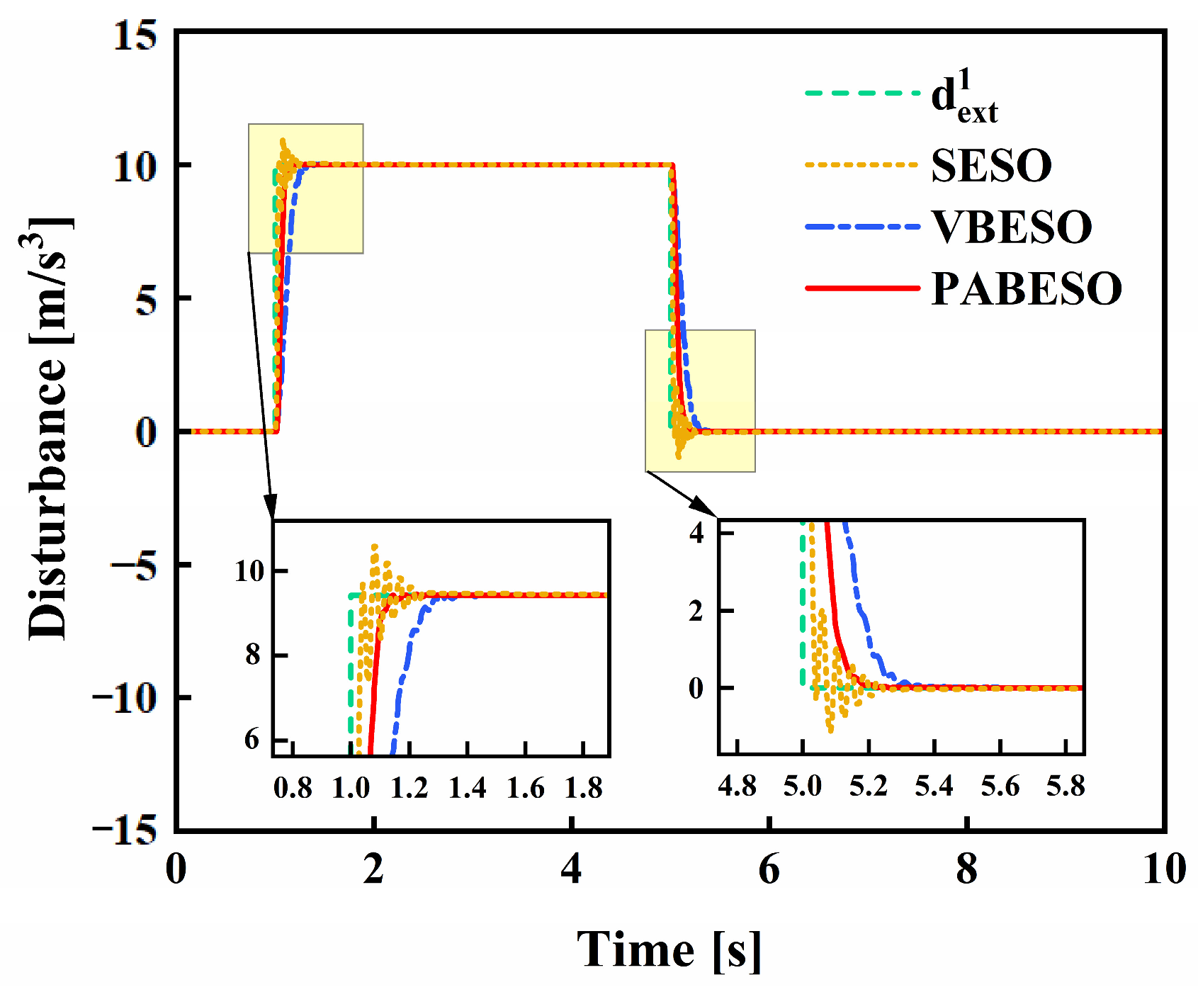
This case evaluates the transient estimation performance of the observers under a sudden, persistent disturbance. A step disturbance $d_{ext}^1=10$ for $1\le t<5 \mathrm{s}$ is applied to emulate an abrupt external load.

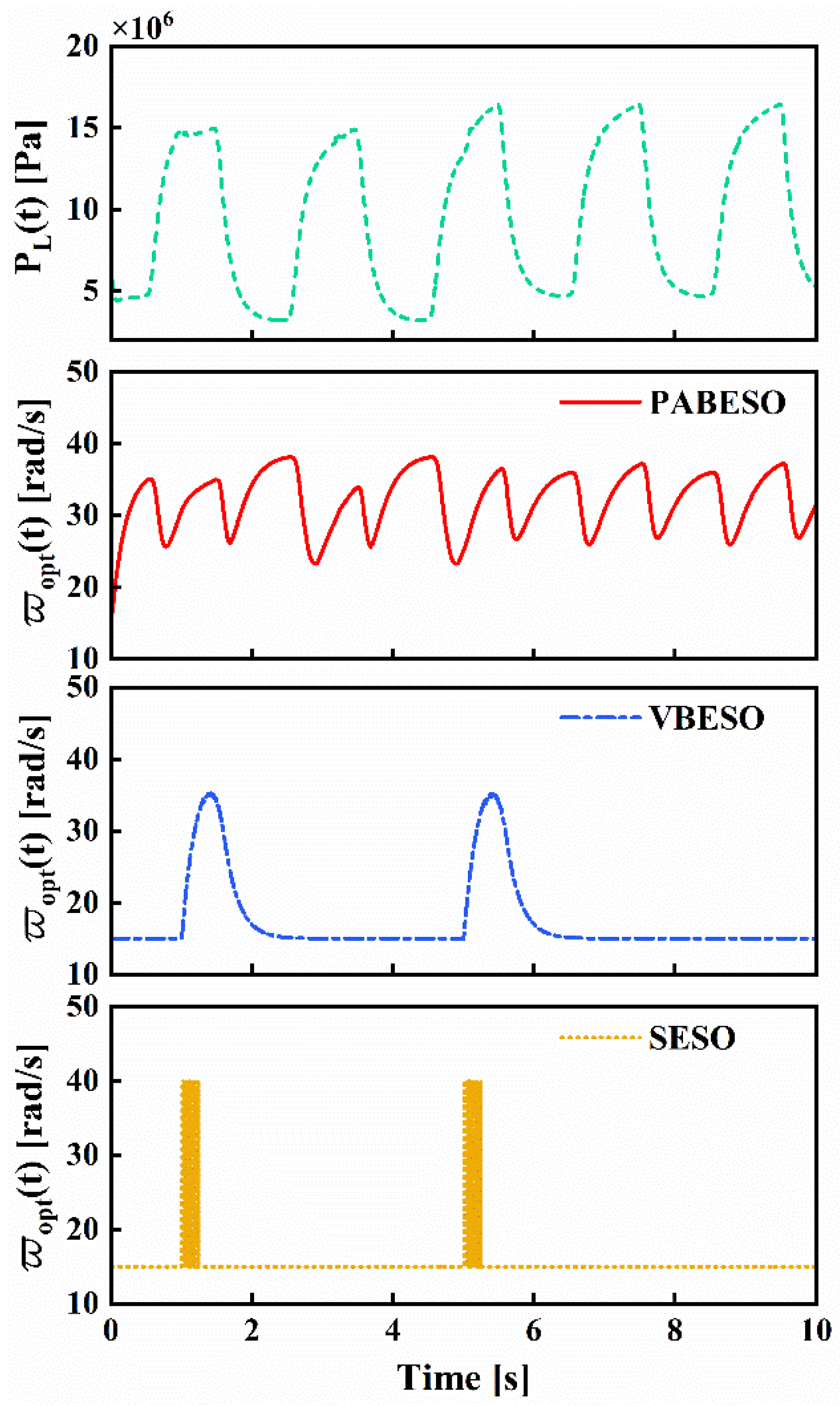
The step disturbance test confirms that the PABESO bridges the causality gap: its physical-state feedforward mechanism uses the load pressure to enable instantaneous disturbance estimation. As Figure 3 reveals, the PABESO’s bandwidth ${\varpi }_{opt}(t)$ is dynamically and nonlinearly coupled to the load pressure $P_L(t)$, enabling it to proactively raise gain concurrent with the disturbance, eliminating the latency inherent in error-feedback adaptation. In contrast, the bandwidths of the conventional observers are decoupled from the core system dynamics. The VBESO bandwidth exhibits a phase-lagged response, while the SESO operates with an error-triggered switching logic, producing a discontinuous square-wave profile that lacks both smoothness and dynamic adaptation.

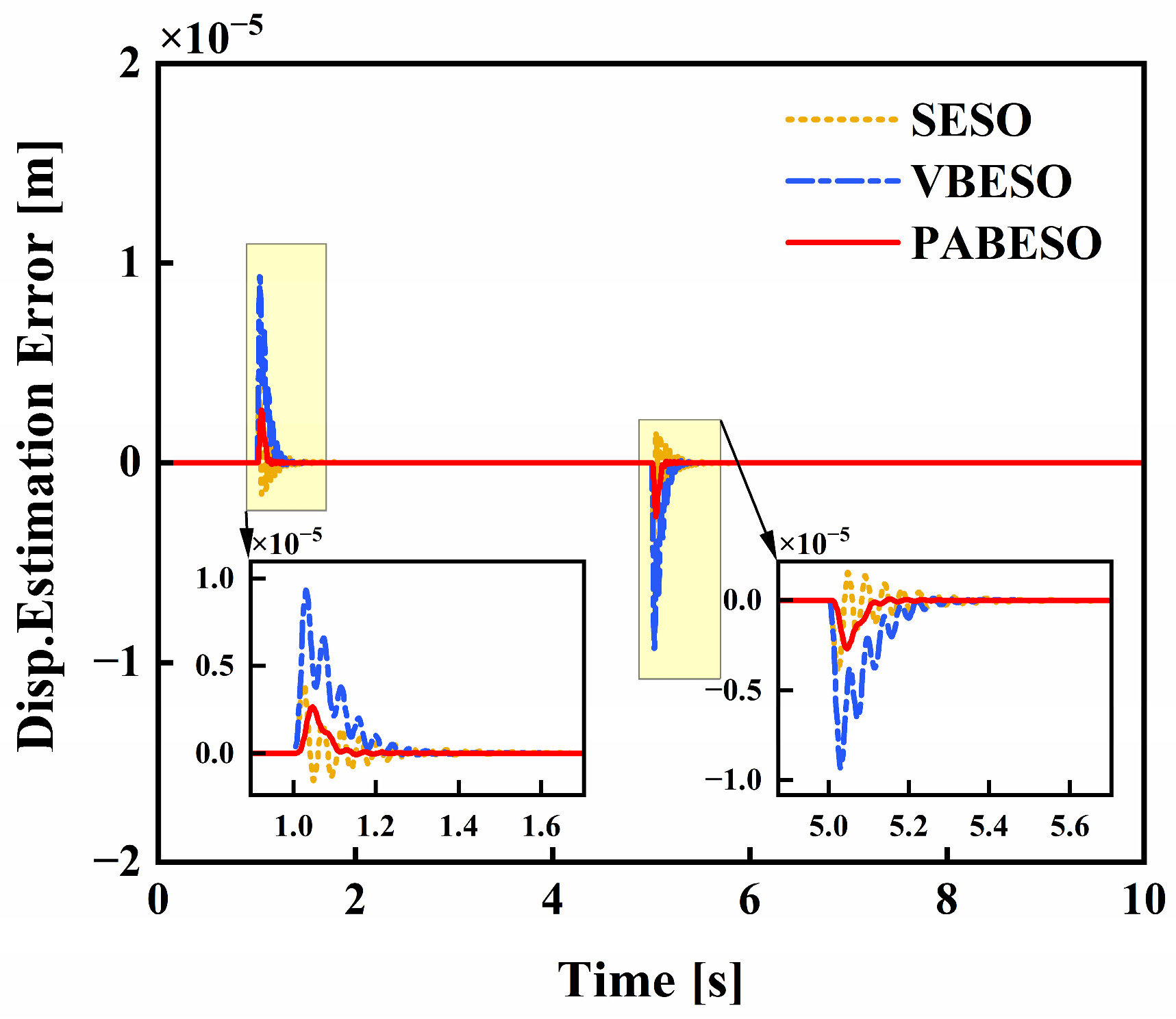
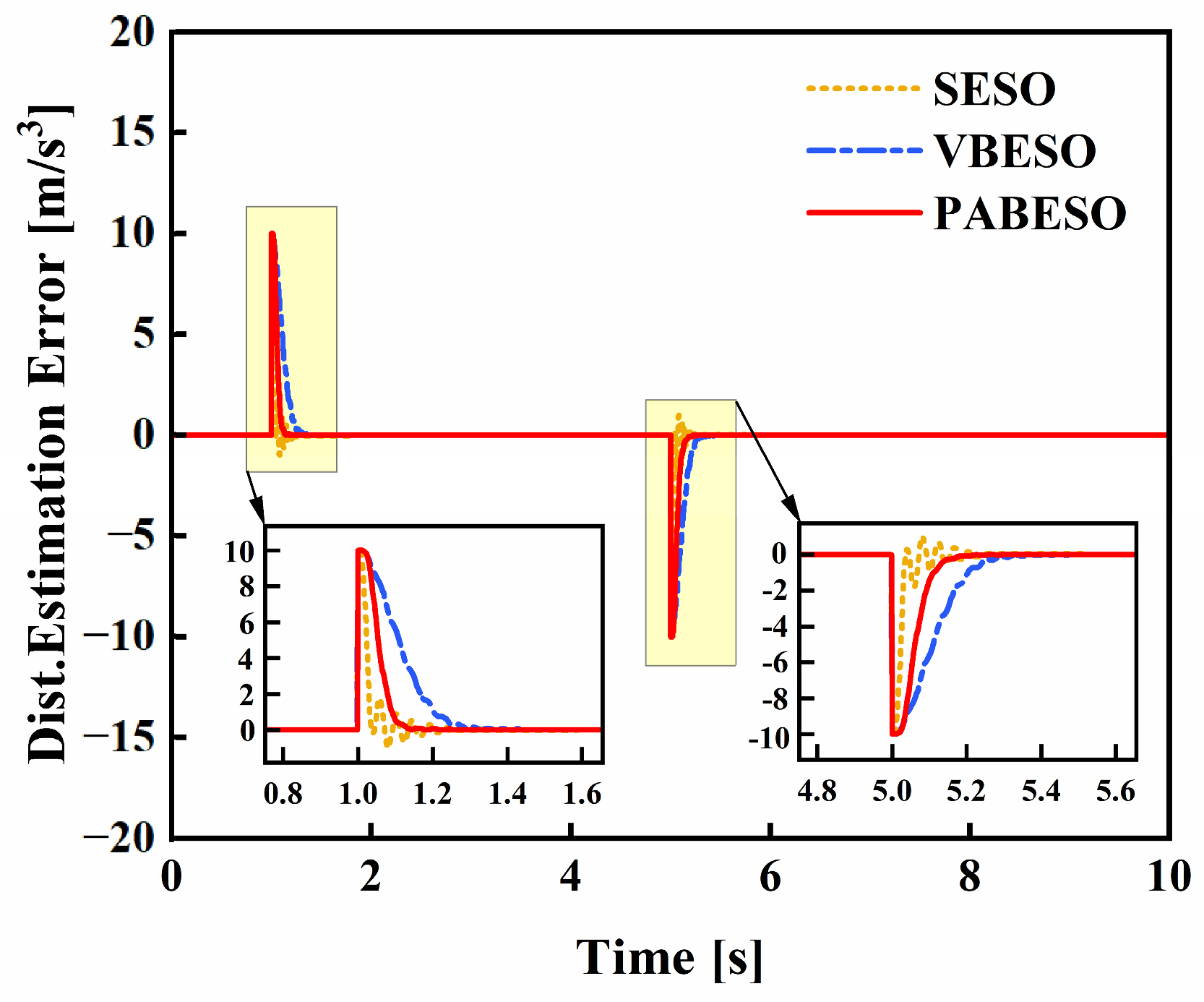
This proactive mechanism translates into definitive performance gains. As quantified in

Table 2. Comparison of estimation performance under step disturbance.

Performance Metric	SESO	VBESO	PABESO
PE of Displacement Estimation $\mathrm{m}$	$4.01\times {10}^{-6}$	$9.31\times {10}^{-6}$	$2.63\times {10}^{-6}$
CT of Disturbance Estimation $\mathrm{s}$	0.14	0.24	0.102
OS of Disturbance Estimation $(\%)$	10.1	0.15	0.17
IAE of Disturbance Estimation $\mathrm{N}\cdot \mathrm{s}$	17.62	13.81	15.41

, the PABESO achieves the fastest disturbance estimation convergence, with a convergence time (CT) of only 0.102 s, which validates the timing advantage claimed in Remark 5. Meanwhile, the lowest peak displacement error (PE) of $2.63\times {10}^{-6} \mathrm{m}$, with a negligible overshoot (OS) of 0.17%, confirms the UUB stability guarantee in Theorem 1. Figure 4 visually confirms this rapid and accurate state estimation, while Figure 5 shows its disturbance estimate ${\mathrm{z}}_4(t)$ smoothly and closely tracking the true disturbance, with an error that decays rapidly and without oscillation (Figure 6). Together, these results depict a well-damped, high-fidelity estimation dynamic.

In contrast, the error-feedback observers are penalized by their reliance on the lagging observation error. For the VBESO, this reliance imposes an inherent hydraulic-to-mechanical delay before the disturbance is perceived as an observation error. This inherent wait results in the slowest convergence (CT = 0.24 s) and the highest peak displacement error (PE = $9.31\times {10}^{-6} \mathrm{m}$), fundamentally crippling its transient response. The SESO attempts to break this wait through aggressive switching, yet its abrupt, error-triggered action merely substitutes delay with instability, causing severe overshoot (OS = 10.10%) and oscillatory transients (Figure 6). This inescapable compromise between agility and robustness underscores the fundamental limitation of reacting to the lagging observation error—a limitation that the PABESO’s physical-state feedforward successfully circumvents.

Case 2: Robustness to Measurement Noise

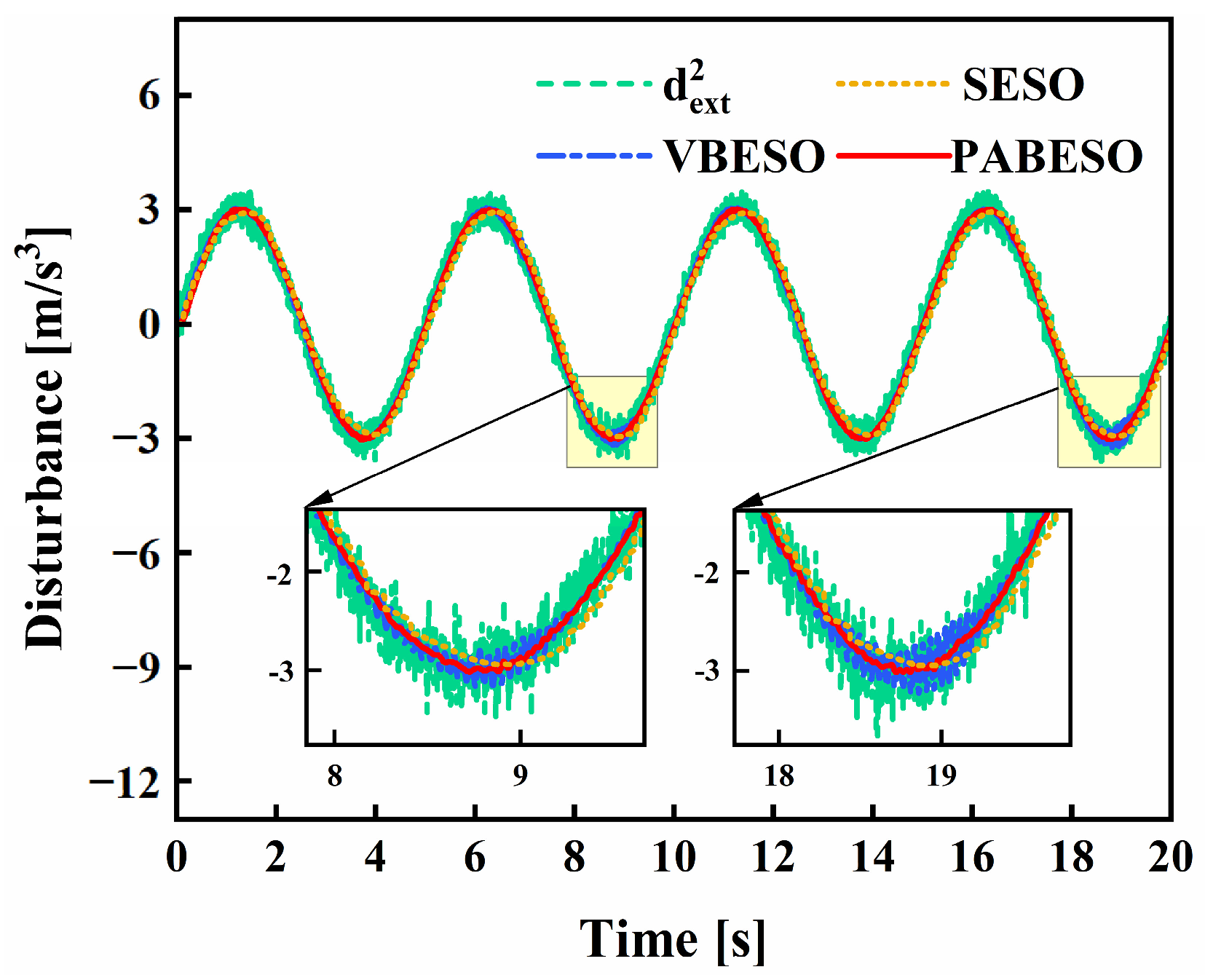
This case evaluates the observer’s steady-state accuracy, noise rejection, and smooth adaptation under sustained oscillatory disturbances with stochastic noise. The compound disturbance is defined as $d_{ext}^2(t)=3\sin (0.4\pi t)+0.1\cdot n(t)$, where $n(t)~\mathcal{N}(0,1)$ is Gaussian white noise, emulating realistic multi-frequency uncertainties.

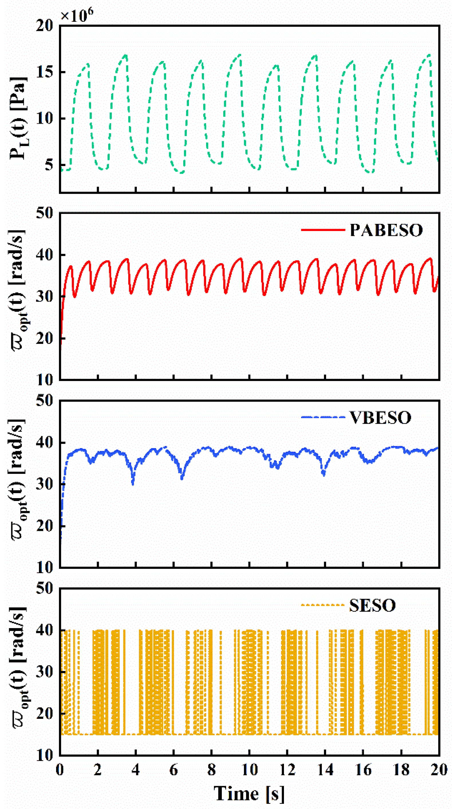
The PABESO’s advantage is again evident in Figure 7, and it exhibits a smooth, continuous, and rhythmic adaptive profile, attributed to its feedforward tuning mechanism directly based on $P_L(t)$. In contrast, the VBESO’s bandwidth exhibits high-frequency jitter and phase lag as its error-feedback loop amplifies and couples noise. The SESO exhibits a fundamentally incompatible bang–bang dynamic, incapable of finely tracking continuous system dynamics and leading to significant errors.

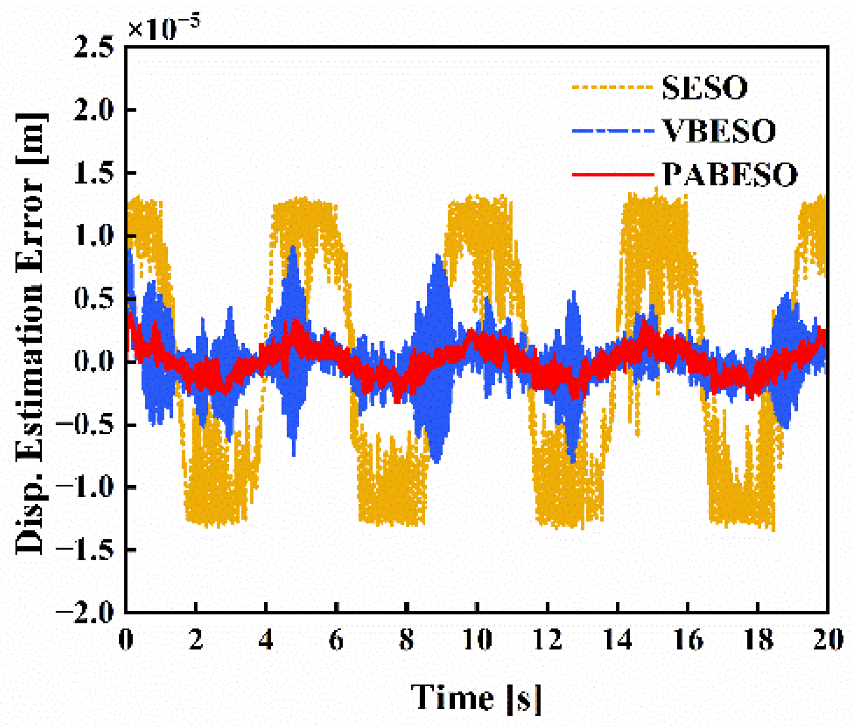
This divergence translates into definitive performance differences in displacement estimation. As shown in Figure 8 and quantified in

Table 3. Comparison of estimation performance under compound disturbance.

Performance Metric	SESO	VBESO	PABESO
RMSE of Displacement Estimation $(\mathrm{m})$	$8.82\times {10}^{-6}$	$2.23\times {10}^{-6}$	$1.22\times {10}^{-6}$
$\left|Max\right|$ of Displacement Estimation $(\mathrm{m})$	$1.38\times {10}^{-5}$	$9.2\times {10}^{-6}$	$3.81\times {10}^{-6}$
RMSE of Disturbance Estimation $(\mathrm{m}/{\mathrm{s}}^3)$	1.21	0.44	0.32
$\left|Max\right|$ of Disturbance Estimation $(\mathrm{m}/{\mathrm{s}}^3)$	2.03	1.53	0.76

, the PABESO achieves the lowest RMSE ($1.22\times {10}^{-6} \mathrm{m}$) and smallest maximum absolute error ($\left|Max\right|$) of $3.81\times {10}^{-6} \mathrm{m}$ in displacement estimation, demonstrating superior steady-state accuracy and further validating the UUB stability guarantee under measurement noise.

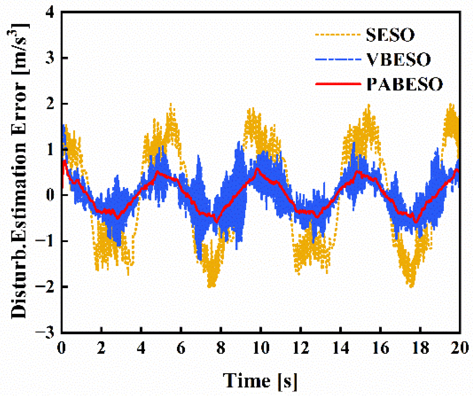
For disturbance estimation, the PABESO accurately tracks the amplitude and phase of the true sinusoidal component with the smoothest trajectory, while effectively suppressing high-frequency noise (Figure 9). The disturbance estimation error in Figure 10 further confirms its fast convergence and small steady-state fluctuation. Quantitatively, Table 3 shows that the PABESO achieves the lowest RMSE ($0.32 \mathrm{m}/{\mathrm{s}}^3$) and the lowest $\left|Max\right|$ ($0.76 \mathrm{m}/{\mathrm{s}}^3$) for disturbance estimation, outperforming both the SESO and VBESO across all metrics.

5.2. Closed-Loop Verification: From Disturbance Estimation to Adaptive Constraint Control

Building upon the high-fidelity disturbance estimate $z_4(t)$ delivered by the PABESO, this section validates how this information enables disturbance-adaptive constraint control. Specifically, four controllers with varying degrees of reliance on $z_4(t)$ are compared under the same PABESO observer, establishing a controlled progression from unconstrained to adaptive constraint enforcement:

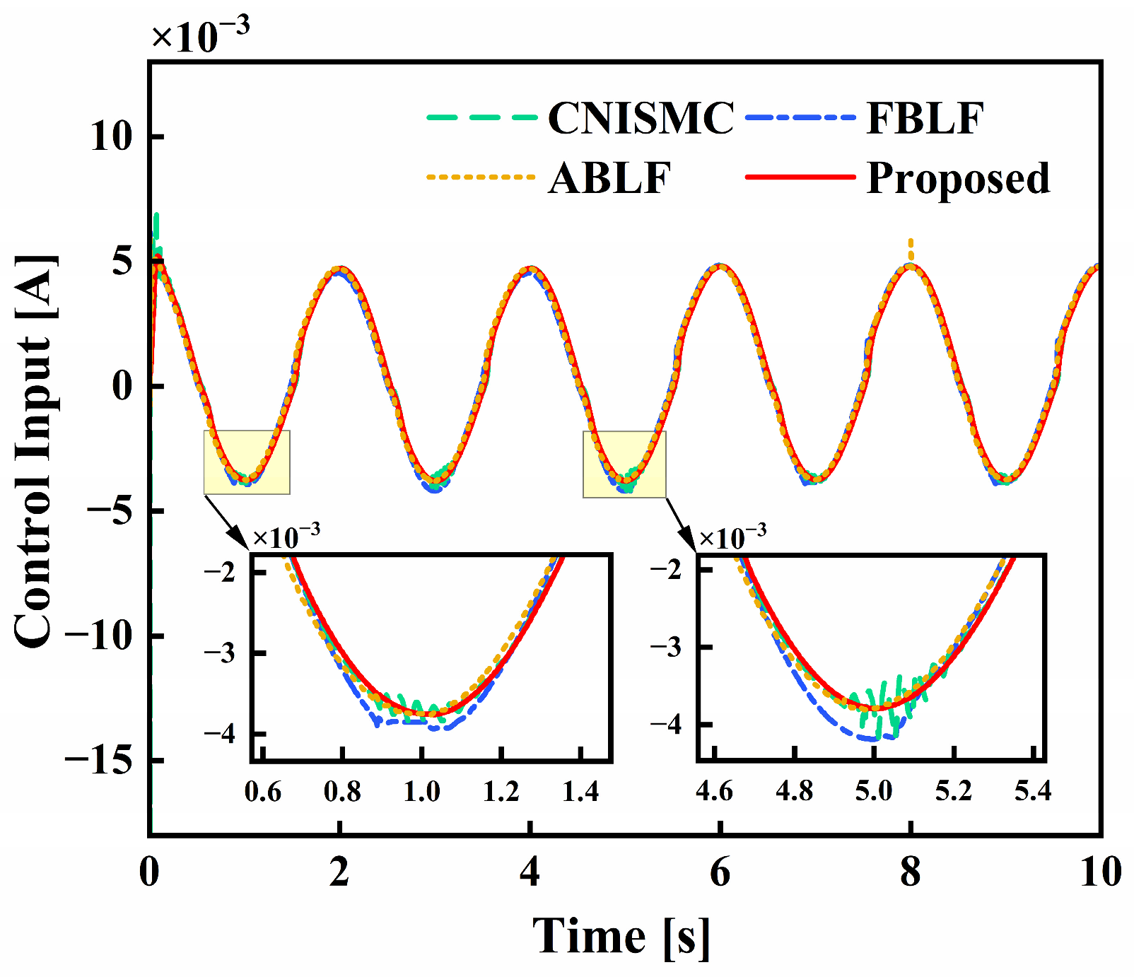
(1) Cascaded nonlinear integral sliding mode control (CNISMC): [37] A robust sliding mode structure with nonlinear integral surfaces and a variable-speed reaching law, where $c_1=300$, $c_2=160$, $k_1=k_2=1\times {10}^4$, $\alpha =0.5$, $\beta =0.05$.

(2) CFBC with a fixed barrier (FBLF): Enforces safety via a static constraint boundary $k=0.02$, effectively ignoring $z_4(t)$ for constraint management.

(3) Adaptive BLF without $d_{phy}(t)$ (ABLF): Same as the proposed controller, but without the $d_{phy}(t)$ feedforward term in (27). It retains the PABESO and the adaptive boundary $k(t)$.

(4) The proposed DBLF-CFBC (Proposed): Our co-designed controller that actively embeds $z_4(t)$ into its disturbance-adaptive boundary $k(t)$ to preemptively manage constraints. The disturbance-adaptive boundary is defined with $k_0=0.05$, ${\lambda }_c=5$, ${\mu }_c=0.0001$, $k_{\infty }=0.008$.

To ensure a strictly controlled comparison, all shared parameters across the controllers are coordinated to a common baseline. The feedback gains are set as $K_1=50$, $K_2=80$, $K_3=300$; the command filter parameters are ${\varsigma }_1={\varsigma }_2=0.7$, ${\omega }_{n1}=50$, ${\omega }_{n2}=50$, ${\varrho }_1=5,{\varrho }_2=10$; and the time constant is $\tau =0.2$ with a derivative gain $K_f=0.01$.

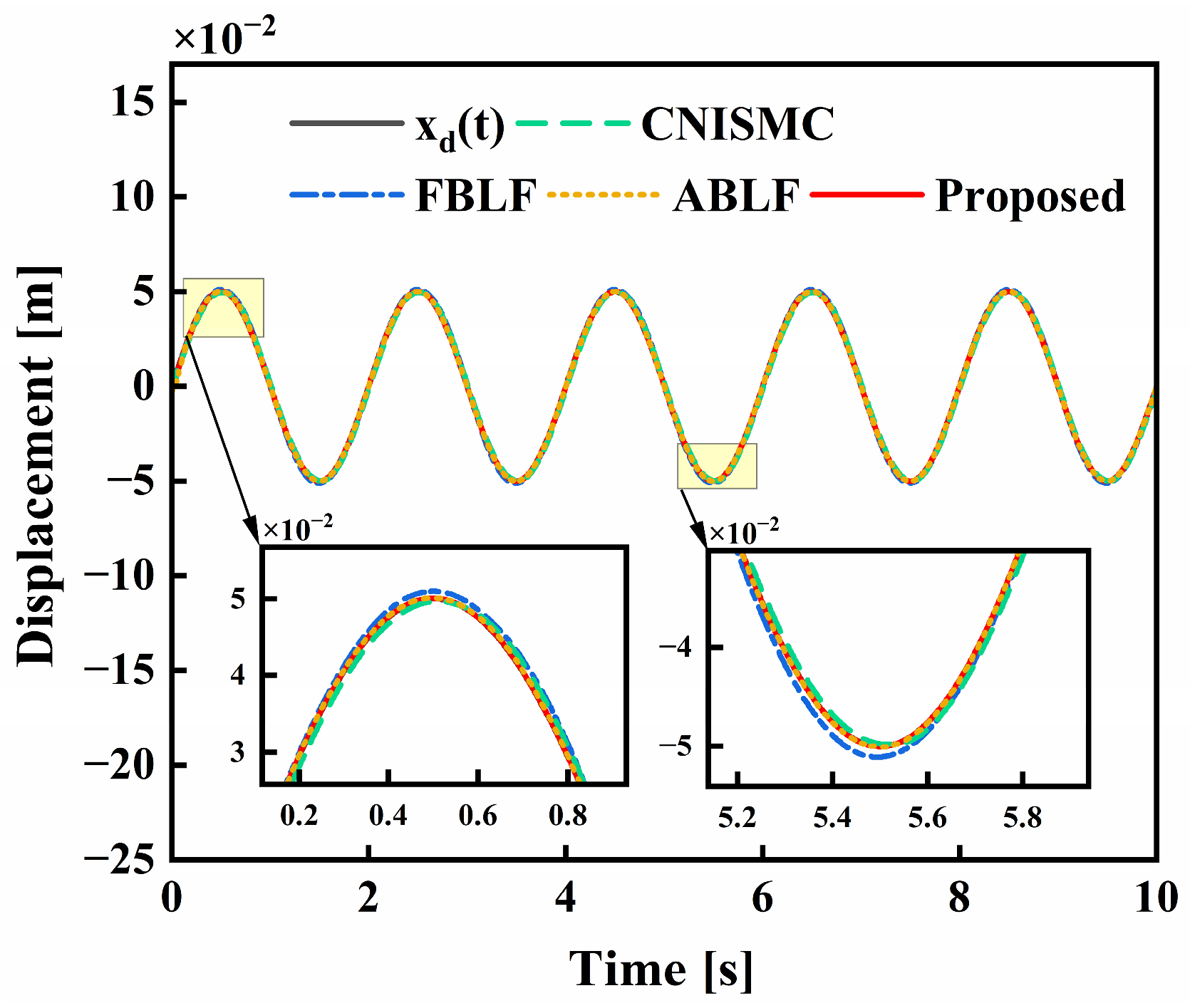
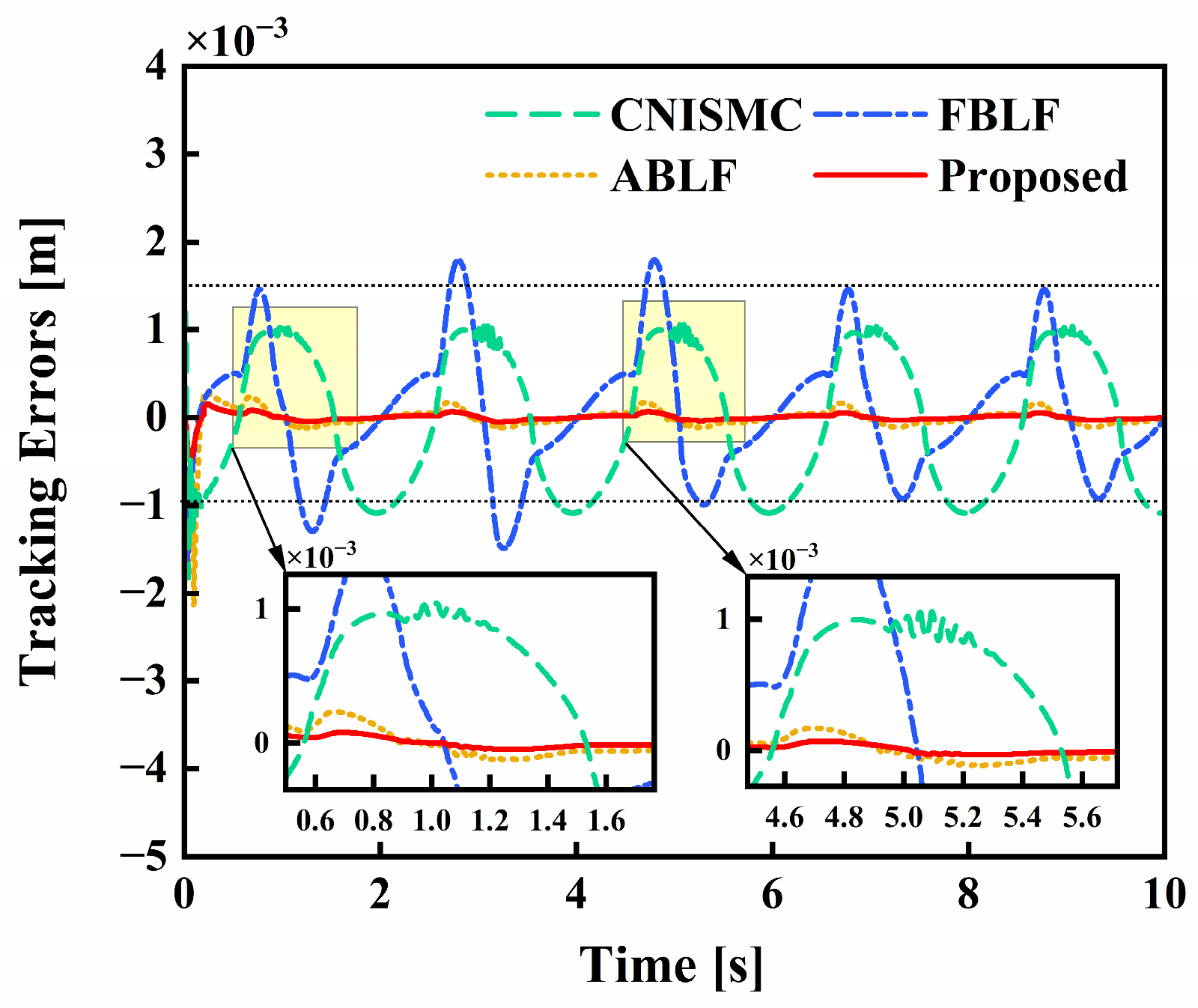
The closed-loop response to a step disturbance $d_{ext}^1=10$ for $1\le t<5 \mathrm{s}$ is shown in Figure 11, Figure 12 and Figure 13, with quantitative metrics in

Table 4. Control performance comparison under step disturbance.

Performance Metric	CNISMC	FBLF	ABLF	Proposed
RMSE of Tracking Error $\mathrm{m}$	$8.06\times {10}^{-4}$	$7.35\times {10}^{-4}$	$4.24\times {10}^{-4}$	$5.10\times {10}^{-5}$
IAE of Tracking Error $(\mathrm{m}\cdot \mathrm{s})$	3.76	2.94	0.57	0.14
$\mathrm{S}\mathrm{t}\mathrm{d}$ of Control Input $\mathrm{A}$	$3.15\times {10}^{-3}$	$3.10\times {10}^{-3}$	$3.08\times {10}^{-3}$	$3.03\times {10}^{-3}$
IAE of Control Input $(\mathrm{A}\cdot \mathrm{s})$	13.99	13.99	13.95	13.81

. Compared with CNISMC, FBLF and ABLF, the proposed controller achieves the smallest tracking error and IAE, reducing both metrics by at least one order of magnitude. As shown in Figure 11, the displacement trajectory of the proposed controller closely follows the desired signal, whereas the other controllers exhibit visible deviations during the disturbance period.

The distinct behaviors of the four controllers are evident in the tracking error trajectories (Figure 12). CNISMC exhibits a larger error amplitude with severe high-frequency chattering at the peaks, particularly during the disturbance period. The FBLF’s fixed barrier induces a nonlinear struggle, resulting in a severely amplified and prolonged tracking error throughout the disturbance. ABLF significantly reduces the tracking error compared to FBLF, but still exhibits noticeable chattering due to the absence of $d_{phy}(t)$ feedforward. In contrast, the proposed controller converges rapidly and remains smooth. This superior performance is attributed to the proactive relaxation of the adaptive boundary $k(t)$, driven by the feedforward estimate $z_4(t)$, confirming the effectiveness of the proposed disturbance-adaptive boundary law. This coupling decouples safety enforcement from transient dynamics, allowing for smooth recovery.

The analysis of the control inputs (Figure 13) confirms that this is achieved through intelligent coordination, not increased effort. All controllers expend comparable total energy (similar IAE of control input), yet the proposed controller exhibits the smoothest input (lowest std) and achieves the lowest cumulative tracking error. Thus, the step disturbance test confirms the closed-loop synergy of the physics-aware design. By linking disturbance estimation to adaptive constraint enforcement, the framework enables the ASEHA to reconcile high tracking accuracy with strict safety, resolving a central challenge in its control.

6. Conclusions

This study demonstrates that a physical-state feedforward approach effectively reduces the latency inherent in error-feedback adaptation in electro-hydraulic control. The approach integrates a pressure-adaptive bandwidth ESO (PABESO), a disturbance-adaptive constraint controller, and a structured disturbance-separation architecture within a co-designed framework. Quantitative comparisons show that the PABESO achieves 2.3 times faster disturbance estimation convergence (0.102 s) than conventional error-feedback observers. The proposed controller reduces tracking error RMSE by an order of magnitude ($5.10 \times {10}^{-5}\mathrm{m}$) compared to methods without disturbance-adaptive boundaries, and these improvements are obtained without increased control effort (IAE of 13.81 A·s). These results suggest that integrating physical-state feedforward into observer-based control is a promising direction for active suspension systems requiring both fast disturbance rejection and strict constraint satisfaction.

References

1. Du, M.; Zhao, D.; Ni, T.; Ma, L.; Du, S. Output feedback control for active suspension electro-hydraulic actuator systems with a novel sampled-data nonlinear extended state observer. IEEE Access 2020, 8, 128741–128756. [Google Scholar] [CrossRef]
2. Wang, W.; Liu, S.; Zhao, D. Low-Complexity Error-Surface Prescribed Performance Control for Nonlinear Uncertain Single-Rod Electro-Hydraulic System. IEEE Trans. Control Syst. Technol. 2024, 32, 2402–2409. [Google Scholar] [CrossRef]
3. Ren, X.; Guo, Q.; Li, T. Initial condition-free prescribed performance fault-tolerant control of electro-hydraulic servo systems with state constraints. Nonlinear Dyn. 2025, 113, 11723–11743. [Google Scholar] [CrossRef]
4. Gao, Z. Scaling and bandwidth-parameterization based controller tuning. In Proceedings of the 2003 American Control Conference; IEEE: Piscataway, NJ, USA, 2003; Volume 6, pp. 4989–4996. [Google Scholar] [CrossRef]
5. Zhang, J.; Cui, C.; Gu, S.; Wang, T.; Zhao, L. Trajectory tracking control of pneumatic servo system: A variable gain ADRC approach. IEEE Trans. Cybern. 2023, 53, 6977–6986. [Google Scholar] [CrossRef] [PubMed]
6. Zhang, Y.; Liang, X.; Li, D.; Ge, S.S.; Gao, B.; Chen, H. Barrier lyapunov function-based safe reinforcement learning for autonomous vehicles with optimized backstepping. IEEE Trans. Neural Netw. Learn. Syst. 2024, 35, 2066–2080. [Google Scholar] [CrossRef] [PubMed]
7. Rath, J.J.; Defoort, M.; Sentouh, C.; Karimi, H.R.; Veluvolu, K.C. Output-Constrained Robust Sliding Mode Based Nonlinear Active Suspension Control. IEEE Trans. Ind. Electron. 2020, 67, 10652–10662. [Google Scholar] [CrossRef]
8. Xia, L.; Yang, L.; Li, W.; Wang, W.; Zhang, J. Discrete Bi-Bandwidth Extended State Observer for Systems with Measurement Noise. IEEE Trans. Ind. Electron. 2024, 71, 7796–7805. [Google Scholar] [CrossRef]
9. Zuo, Y.; Ge, X.; Zheng, Y.; Chen, Y.; Wang, H.; Woldegiorgis, A.T. An adaptive active disturbance rejection control strategy for speed-sensorless induction motor drives. IEEE Trans. Transp. Electrif. 2022, 8, 3336–3348. [Google Scholar] [CrossRef]
10. Zhang, S.; Qi, X.; Yang, S. An extended state observer with adjustable bandwidth for measurement noise. J. Syst. Eng. Electron. 2024, 35, 233–241. [Google Scholar] [CrossRef]
11. Sun, C.; Fang, J.; Wei, J.; Hu, B. Nonlinear motion control of a hydraulic press based on an extended disturbance observer. IEEE Access 2018, 6, 18502–18510. [Google Scholar] [CrossRef]
12. Merritt, H.E.; Pomper, V. Hydraulic control systems. J. Appl. Mech. 1968, 35, 200. [Google Scholar] [CrossRef]
13. Wu, Q.; Wang, Z.; Chen, Y.; Wu, H. Barrier lyapunov function-based fuzzy adaptive admittance control of an upper limb exoskeleton using RBFNN compensation. IEEE/ASME Trans. Mechatron. 2025, 30, 3–14. [Google Scholar] [CrossRef]
14. Guo, X.-G.; Xu, W.-D.; Wang, J.-L.; Park, J.H.; Yan, H. BLF-based neuroadaptive fault-tolerant control for nonlinear vehicular platoon with time-varying fault directions and distance restrictions. IEEE Trans. Intell. Transp. Syst. 2022, 23, 12388–12398. [Google Scholar] [CrossRef]
15. Tee, K.P.; Ge, S.S.; Tay, E.H. Barrier lyapunov functions for the control of output-constrained nonlinear systems. Autom. J. IFAC 2009, 45, 918–927. [Google Scholar] [CrossRef]
16. Jia, T.; Pan, Y.; Liang, H.; Lam, H.-K. Event-Based Adaptive Fixed-Time Fuzzy Control for Active Vehicle Suspension Systems with Time-Varying Displacement Constraint. IEEE Trans. Fuzzy Syst. 2022, 30, 2813–2821. [Google Scholar] [CrossRef]
17. Wang, X.; Zhao, X.; Niu, B.; Wang, Y.; Zhang, J.; Zong, G. Adaptive fault tolerant tracking control for output constrained nonlinear systems using a novel BLF method. IEEE Trans. Syst. Man Cybern. Syst. 2025, 55, 2590–2598. [Google Scholar] [CrossRef]
18. Zhao, L.; Yu, J.; Wang, Q.-G. Finite-Time Tracking Control for Nonlinear Systems via Adaptive Neural Output Feedback and Command Filtered Backstepping. IEEE Trans. Neural Netw. Learn. Syst. 2021, 32, 1474–1485. [Google Scholar] [CrossRef] [PubMed]
19. Zhang, X.; Lin, Y. Adaptive control of nonlinear time-delay systems with application to a two-stage chemical reactor. IEEE Trans. Autom. Control 2015, 60, 1074–1079. [Google Scholar] [CrossRef]
20. Hao, R.; Wang, H.; Liu, S.; Yang, M.; Tian, Z. Multi-objective command filtered adaptive control for nonlinear hydraulic active suspension systems. Nonlinear Dyn. 2021, 105, 1559–1579. [Google Scholar] [CrossRef]
21. Wang, T.; Li, Y. Neural-network adaptive output-feedback saturation control for uncertain active suspension systems. IEEE Trans. Cybern. 2022, 52, 1881–1890. [Google Scholar] [CrossRef] [PubMed]
22. Dong, W.; Farrell, J.A.; Polycarpou, M.M.; Djapic, V.; Sharma, M. Command filtered adaptive backstepping. IEEE Trans. Control Syst. Technol. 2012, 20, 566–580. [Google Scholar] [CrossRef]
23. Qin, Y.; Zhao, D.; Zhang, W.; Deng, Y. Improved Active Disturbance Rejection Control and Parameter Setting for Position Tracking of Active Suspension Electro-Hydraulic Servo Actuator. IEEE/ASME Trans. Mechatron. 2024, 30, 1971–1982. [Google Scholar] [CrossRef]
24. Han, J. From PID to active disturbance rejection control. IEEE Trans. Ind. Electron. 2009, 56, 900–906. [Google Scholar] [CrossRef]
25. Yao, J.; Deng, W.; Jiao, Z. Adaptive control of hydraulic actuators with LuGre model-based friction compensation. IEEE Trans. Ind. Electron. 2015, 62, 6469–6477. [Google Scholar] [CrossRef]
26. Zuo, Y.; Zhu, J.; Jiang, W.; Xie, S.; Zhu, X.; Chen, W.-H. Active disturbance rejection controller for smooth speed control of electric drives using adaptive generalized integrator extended state observer. IEEE Trans. Power Electron. 2023, 38, 4323–4334. [Google Scholar] [CrossRef]
27. Cao, H.; Deng, Y.; Zuo, Y.; Li, H.; Wang, J.; Liu, X. Improved ADRC with a cascade extended state observer based on quasi-generalized integrator for PMSM current disturbances attenuation. IEEE Trans. Transp. Electrif. 2024, 10, 2145–2157. [Google Scholar] [CrossRef]
28. Yao, B.; Bu, F.; Reedy, J.; Chiu, G.T.-C. Adaptive robust motion control of single-rod hydraulic actuators: Theory and experiments. IEEE/ASME Trans. Mechatron. 2000, 5, 79–91. [Google Scholar] [CrossRef]
29. Alleyne, A.; Liu, R. A simplified approach to force control for electro-hydraulic systems. Control Eng. Pract. 2000, 8, 1347–1356. [Google Scholar] [CrossRef]
30. Gu, W.; Yao, J.; Yao, Z.; Zheng, J. Output feedback model predictive control of hydraulic systems with disturbances compensation. ISA Trans. 2019, 88, 216–224. [Google Scholar] [CrossRef] [PubMed]
31. Cui, B.; Zhao, G.; Xia, Y.; Wang, P.; Zhang, Y. A variable-bandwidth extended state observer for nonlinear systems with measurement noise. IEEE Trans. Ind. Electron. 2025, 72, 1946–1957. [Google Scholar] [CrossRef]
32. Li, Y.; Tong, S. Command-filtered-based fuzzy adaptive control design for MIMO-switched nonstrict-feedback nonlinear systems. IEEE Trans. Fuzzy Syst. 2017, 25, 668–681. [Google Scholar] [CrossRef]
33. Khalil, H.K.; Grizzle, J.W. Nonlinear Systems, 3rd ed.; Prentice Hall: Upper Saddle River, NJ, USA, 2002. [Google Scholar]
34. Gu, S.; Zhang, J.; Li, Y. Generalized variable gain ADRC for nonlinear systems and its application to delta parallel manipulators. IEEE Trans. Circuits Syst. I 2023, 70, 921–930. [Google Scholar] [CrossRef]
35. Deng, H.; Krstić, M. Stochastic nonlinear stabilization—I: A backstepping design. Syst. Control Lett. 1997, 32, 143–150. [Google Scholar] [CrossRef]
36. Xie, T.; Zhang, H.; Yu, Y.; Li, R. A mutation bandwidth extended state observer for PMSM deadbeat control systems. Electr. Eng. 2025, 107, 14239–14251. [Google Scholar] [CrossRef]
37. Li, Y.; Dong, W.; Bai, J.; Yao, Z.; Bi, Q.; Li, X. Novel cascade sliding mode control of loader electro-hydraulic systems based on improved extended state observers. IEEE Trans. Ind. Electron. 2025, 72, 14314–14324. [Google Scholar] [CrossRef]
Figure 1. Schematic Diagram of the ASEHA.
Actuators 15 00375 g001
Figure 2. Co-designed observer-controller framework.
Actuators 15 00375 g002
Figure 3. Load pressure and observer bandwidth under step disturbance.
Actuators 15 00375 g003
Figure 4. Displacement estimation error under step disturbance.
Actuators 15 00375 g004
Figure 5. Disturbance and its estimate under step disturbance.
Actuators 15 00375 g005
Figure 6. Disturbance estimation error under step disturbance.
Actuators 15 00375 g006
Figure 7. Load pressure and observer bandwidth under compound disturbance.
Actuators 15 00375 g007
Figure 8. Displacement estimation error under compound disturbance.
Actuators 15 00375 g008
Figure 9. Disturbance and its estimate under compound disturbance.
Actuators 15 00375 g009
Figure 10. Disturbance estimation error under compound disturbance.
Actuators 15 00375 g010
Figure 11. Comparison of displacement tracking under the test disturbance.
Actuators 15 00375 g011
Figure 12. Displacement tracking error comparison.
Actuators 15 00375 g012
Figure 13. Control input comparison.
Actuators 15 00375 g013