Data-Based Youla Parameterization for Robust Disturbance Observer Design of VCM Motion Stage

Abstract

Robust disturbance rejection in voice coil motor (VCM) motion stages is often limited by model uncertainties and the difficulty of obtaining accurate plant inverses. To address this issue, this paper develops a data-based Youla parameterization method for designing a robust disturbance observer (DOB) without relying on an analytical plant model. Frequency response data from the VCM stage are measured directly under multiple operating conditions. The Youla parameter Q is expanded using a Laguerre orthogonal basis, and its coefficients are optimized by solving a convex problem that enforces H∞ robust stability and H₂ average tracking error constraints on a finite frequency grid. Experiments on a VCM motion stage demonstrate that the optimized Q filter effectively estimates and rejects electromagnetic noise and other disturbances. A total of 30 groups of data covering the full range of operating conditions were used for optimization, and 10 randomly designed experiments were conducted to validate the controller, with the maximum average error below 0.05%. Repetitive tests were carried out to verify the tracking performance for 1 Hz sinusoidal and triangular signals. The results show that the average RMSEs of the proposed method is 0.87% and 0.59%, respectively, which are lower than those of the ITAE-PID, ADRC and K₀ controllers. Finally, the robustness of the proposed method is further verified by analyzing the sensitivity function of the closed-loop system.

1. Introduction

With the rapid development of fields such as ultra-precision manufacturing [1], precision metrology [2], and biomedicine [3], the demand for motion control systems with both large stroke and high precision continues to grow. VCM-driven motion stages have become core components in these systems because their simple structure, fast dynamic response, high linearity, and absence of cogging force enable centimeter-level travel with micrometer- or even nanometer-level positioning accuracy.

However, in practical operation, VCM motion stages face significant challenges that severely limit their control performance. On the one hand, VCM systems are highly sensitive to disturbances, including external environmental disturbances, internal nonlinearities, and model uncertainties caused by parameter fluctuations during long-term operation [4]. These disturbances can reduce the positioning accuracy and dynamic response capability of the stage, making it difficult to satisfy the increasingly stringent precision requirements of modern industrial applications. On the other hand, as VCM motion stages develop toward miniaturization and integration, the coupling among mechanical, electromagnetic, and thermal fields becomes more complex, which makes it difficult to establish an accurate mathematical model using traditional electromechanical modeling methods.

In response to these challenges, several control methodologies have been proposed for disturbance and uncertainty attenuation. Representative techniques include DOBs [5,6], extended state observers (ESOs) [7,8], and uncertainty and disturbance estimators (UDEs) [9], all of which are designed to actively estimate and compensate for unmodeled dynamics and external perturbations. Yang et al. developed a composite hierarchical control system incorporating a DOB and an error-based ADRC to address disturbances and model uncertainties across multiple frequency bands [10]. Naghdi et al. proposed a cooperative control strategy combining a fuzzy extended state observer (FESO) with a robust controller, this strategy can estimate hysteresis, nonlinearities, model uncertainties, and external disturbances, thereby demonstrating markedly improved performance [11]. In addition, Yue et al. introduced an online H∞ tracking control method that uses real-time measurement data and is tailored to systems subject to time delays and disturbances [12]. Although these methods are effective, many rely on real-time estimation and implicitly assume that a precise model is either available or unnecessary. This dependence ties performance to observer bandwidth and leaves offline a priori information underused.

In contrast, Li et al. [13] focused on the Q-filter structure and implemented a non-binomial filter tuned through data-driven gradient optimization. Liu et al. [14] developed a modified data-driven DOB with a parallel Q-filter structure and an interchanged signal-point design, which significantly suppressed quadrant glitches in a ball-screw feed-drive system while maintaining robust stability. As a more general solution, Zheng et al. [15] proposed a learning-based disturbance observer that integrates H∞ optimization with iterative learning to handle MIMO and nonminimum-phase systems without requiring a plant inverse. Further advances include the performance robustness decoupling achieved by Feng et al. [16] through a generalized internal model control structure and the systematic coordination of multiple controllers by Xu et al. [17] using Youla parameterization. Youla parameterization has also been extended to the design of an error-based observer (EOB) [18] and to DISO systems [19]. Collectively, these methods provide strong theoretical guarantees and show considerable potential, making them an important direction in current research.

The main contributions of this paper are summarized as follows:

(1)

A data-based controller synthesis method is developed from measured input-output frequency-response data. Unlike conventional DOB, the proposed method avoids explicit plant modeling and inverse model construction, making it suitable for systems with complex dynamics and plant uncertainties.

(2)

A unified optimization framework is established within the Youla-parameterized stabilization structure. Controller synthesis is formulated as an optimization problem of the Youla parameter, where robustness and performance specifications are simultaneously incorporated into a frequency-domain optimization framework while guaranteeing closed-loop stability throughout the design process.

(3)

Experimental studies on a VCM motion stage validate the effectiveness of the proposed method. Disturbance rejection capability, tracking performance, and robustness are systematically evaluated and compared with those of the baseline K₀, ADRC, and ITAE-PID controllers under plant variations and external disturbances.

The rest of this paper is organized as follows. Section 2 presents the problem formulation. Section 3 introduces the robust DOB control structure. Section 4 describes the data-based control design. Section 5 presents experimental results that demonstrate the effectiveness of the proposed method. Finally, Section 6 concludes the paper.

2. Problem Formulation

2.1. Modeling of the VCM Motion Stage

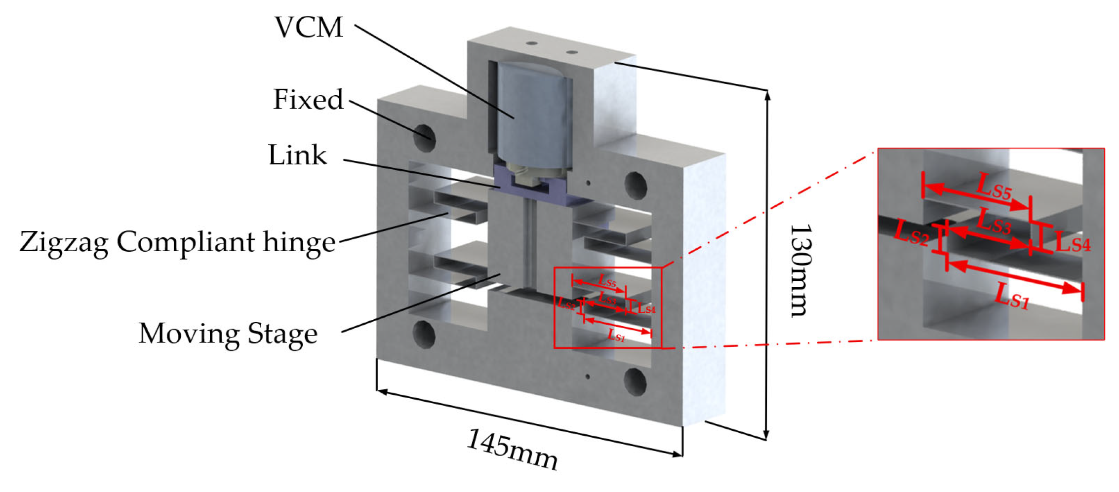
The VCM motion stage, as shown in Figure 1, is directly driven by a VCM to actuate a parallelogram-structured Zigzag flexible guiding mechanism, which achieves friction-less, backlash less and single-degree-of-freedom positioning through elastic deformation. The dynamic model of the motion stage can be expressed as a third-order system, as shown in Equation (1). The total mass of the VCM mover, the link, and the moving stage is denoted as m, the displacement as y, and the viscous damping coefficient of the system as c. The driving force generated by the VCM is F = BIl, where B is the magnetic flux density and l is the effective coil length. The current I satisfies the first-order linear differential equation $\mathrm{L} = {\displaystyle \frac{\mathrm{d}\mathrm{I}}{\mathrm{d}\mathrm{t}}} + \mathrm{RI} = \mathrm{u}-{\mathrm{K}}_{\mathrm{e}}\dot{y}$, with R as the coil resistance and K_e as the back electromotive force constant. The Zigzag flexure hinge provides the equivalent stiffness ${\mathrm{K}}_{\mathrm{z}} = {\displaystyle \frac{5\mathrm{EA}\left({\mathrm{L}}_{\mathrm{s}1}^3 + {\mathrm{L}}_{\mathrm{s}3}^3 +{ \mathrm{L}}_{\mathrm{s}5}^3\right) + 72\mathrm{EI}(1 + \mathsf{\lambda }\left)\right({\mathrm{L}}_{\mathrm{s}1} +{ \mathrm{L}}_{\mathrm{s}3} +{ \mathrm{L}}_{\mathrm{s}5})}{60\mathrm{AI}{\mathrm{E}}^2}}$ of the system, which is obtained through static analysis (see Ref. [20] for details).

$$\mathrm{mL}{\displaystyle \frac{{\mathrm{d}}^{3}y}{\mathrm{d}{\mathrm{t}}^3}}+\left(\mathrm{cL}+\mathrm{mR}\right){\displaystyle \frac{{\mathrm{d}}^{2}y}{\mathrm{d}{\mathrm{t}}^2}}+\left({\mathrm{k}}_{\mathrm{z}}\mathrm{L}+\mathrm{cR}+{\mathrm{B}}^2{\mathrm{l}}^2\right){\displaystyle \frac{\mathrm{d}y}{\mathrm{dt}}}+{ \mathrm{k}}_{\mathrm{z}}\mathrm{Rx}=\mathrm{Blu}.$$

(1)

Remark 1.

In practice, when the VCM operates over a large stroke, the magnetic field distribution becomes non-uniform, causing the force constant K_t = Bl to vary with the mover position y, i.e., K_t = K_t(y). Furthermore, the coil resistance R is temperature-dependent: R(T) = R₀[1 + α (T − T₀)], where α is the temperature coefficient and T₀ is the ambient temperature. Load variations (e.g., different payload masses) affect the total moving mass m and may also change the damping coefficient c. These nonlinear and time-varying characteristics are not explicitly captured in the linear model of Equation (1). Instead, they are implicitly considered in the data-based structure by collecting frequency-response measurements under multiple operating conditions, including different positions, temperatures, and loads. Consequently, the proposed controller design does not rely on an exact analytical model but directly uses these measured data to achieve robust performance.

In this work, the model above is used only as a nominal reference for comparison with model-based methods. The proposed data-based controller design does not rely on any numerical values of m, c, k_z, B, l, R, or L. Instead, it directly uses input-output frequency-domain data acquired from the actual stage.

2.2. Traditional DOB Structure

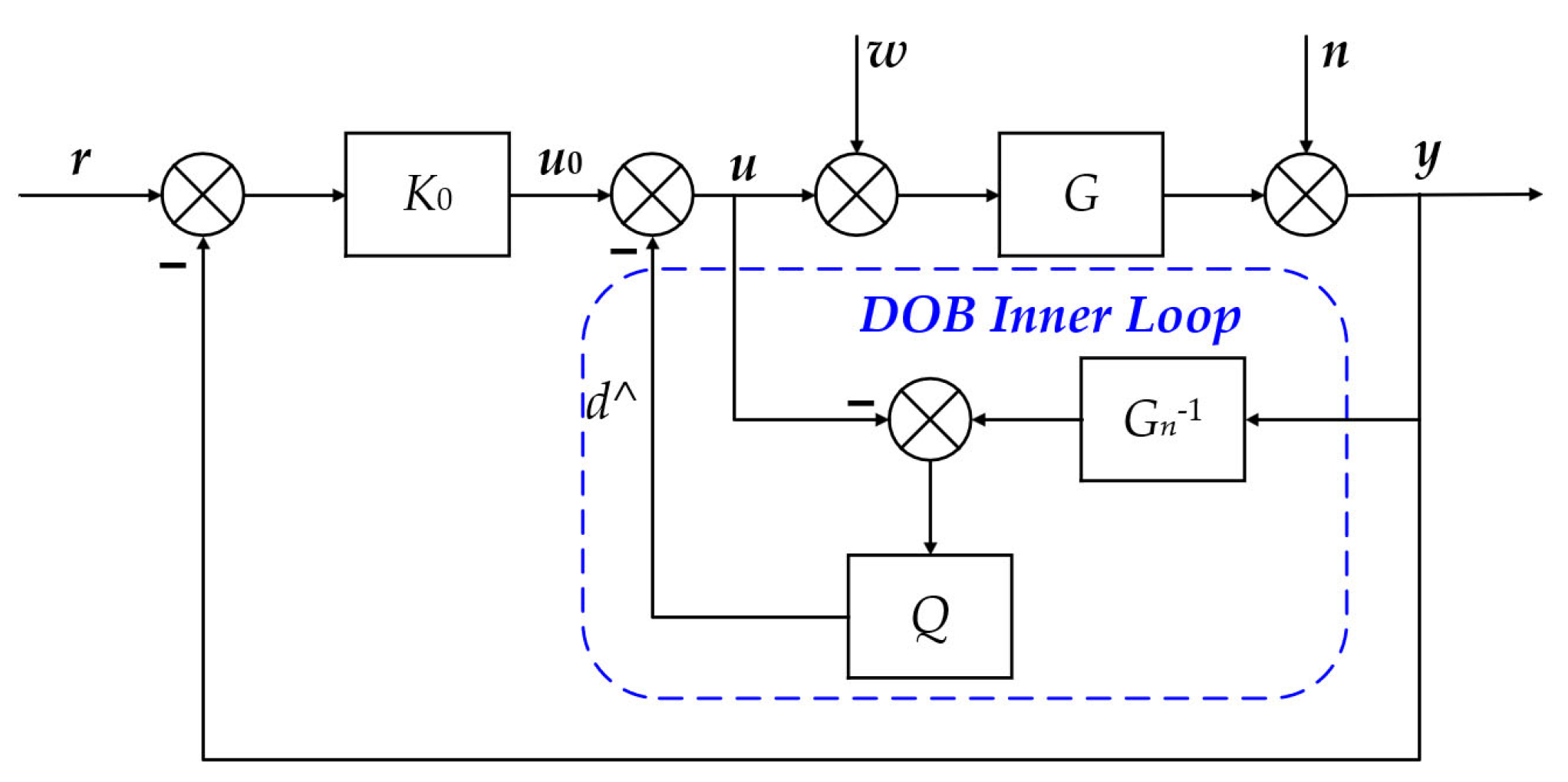
The standard DOB, depicted in Figure 2 (where G is the actual plant, G_n is its nominal model, Q is the low-pass filter, and K₀ is the feedback controller), employs a Q-filter and the inverse of the nominal plant G_n⁻¹, to reconstruct the control input and estimate disturbances. Disturbance w is injected at the plant input, while measurement noise n is superimposed on the sensor output. The closed-loop transfer function from disturbance w to output y is expressed by Equation (2). A properly designed Q-filter is critical for maintaining system robustness against external disturbances and model uncertainties. Q is typically selected as a low-pass filter. A higher bandwidth extends the frequency range of disturbance suppression but also increases the system’s sensitivity to model errors and measurement noise. This trade-off limits the performance of conventional DOBs in environments with strong uncertainties and high-frequency noise. Moreover, the selection of the filter order and cutoff frequency relies on engineering heuristics, lacking a systematic optimization framework. A further implementation challenge lies in solving the inverse model of the plant.

To overcome this limitation, this paper introduces the Youla parameterization, which treats Q as a free parameter. Within a data-based approach, convex optimization is used to simultaneously satisfy robustness and disturbance rejection constraints, thereby yielding an optimal Q.

$${\mathrm{G}}_{\mathit{wy}}={\displaystyle \frac{\mathrm{G}{\mathrm{G}}_{\mathrm{n}}(1-Q)}{{\mathrm{G}}_{\mathrm{n}}\left(1 -Q\right)+\mathrm{GQ} +{\mathrm{K}}_0\mathrm{G}{\mathrm{G}}_{\mathrm{n}}}}.$$

(2)

3. Robust DOB Control Structure

3.1. DOB Design Using Youla Parameterization

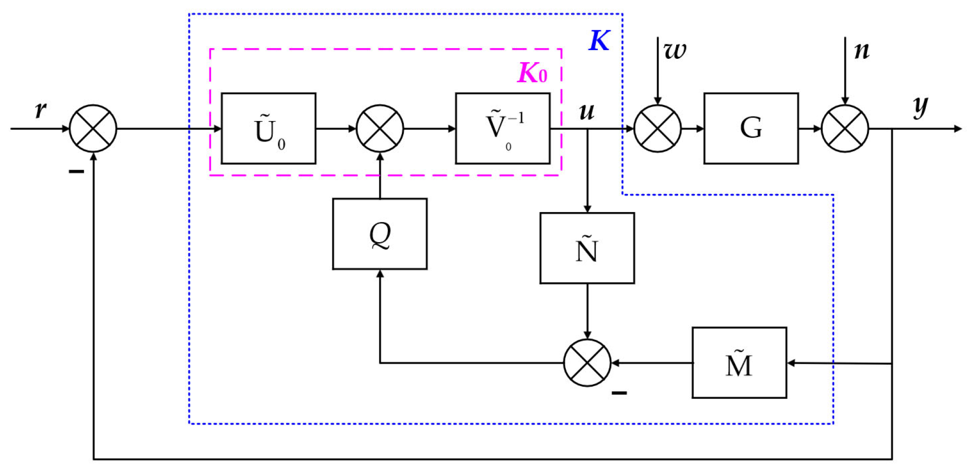
For a unit negative feedback system, the plant G and the controller K can be expressed using left-coprime factorizations over stable rational functions as

$$\mathrm{G}={\stackrel{\mathrm{~}}{ \mathrm{M}}}^{-1}\stackrel{\mathrm{~}}{\mathrm{N}},$$

(3)

$$\mathrm{K} ={ \left({\stackrel{\mathrm{~}}{\mathrm{V}}}_0-Q\stackrel{\mathrm{~}}{\mathrm{N}}\right)}^{-1}\left({\stackrel{\mathrm{~}}{\mathrm{U}}}_0+Q\stackrel{\mathrm{~}}{\mathrm{M}}\right),$$

(4)

where $\stackrel{\mathrm{~}}{\mathrm{M}}$, $\stackrel{\mathrm{~}}{\mathrm{N}}$, ${\stackrel{\mathrm{~}}{\mathrm{U}}}_0$, and ${\stackrel{\mathrm{~}}{\mathrm{V}}}_0$ are stable transfer functions. The initial stabilizing controller ${\mathrm{K}}_0 ={\stackrel{\mathrm{~}}{ \mathrm{V}}}_0^{-1}{\stackrel{\mathrm{~}}{\mathrm{U}}}_0$ is assumed to satisfy the Bezout identity [21]. The family of all internally stabilizing controllers is parameterized by an arbitrary stable Q via Equation (4). It can be represented as the control structure shown in Figure 3.

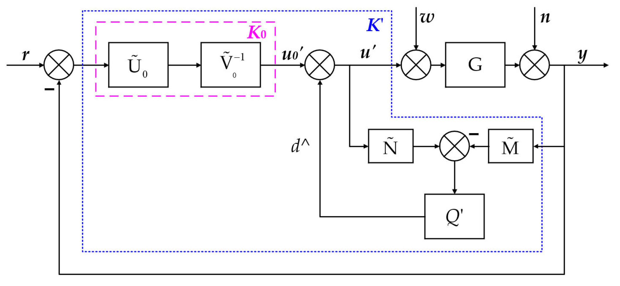
An equivalent block-diagram transformation of Figure 3 yields the controller configuration in Figure 4, where the free parameter becomes $Q^{\prime } = Q{\stackrel{\mathrm{~}}{\mathrm{V}}}_0^{-1}$. The transformation is derived as follows. Starting from Equation (4), multiplying the numerator and denominator on the right by ${\stackrel{\mathrm{~}}{\mathrm{V}}}_0^{-1}$

$${\mathrm{K}}^{\prime }={ \left({\stackrel{\mathrm{~}}{\mathrm{V}}}_0\left(\mathrm{I}-Q\stackrel{\mathrm{~}}{\mathrm{N}}{\stackrel{\mathrm{~}}{\mathrm{V}}}_0^{-1}\right)\right)}^{-1}\left({\stackrel{\mathrm{~}}{\mathrm{U}}}_0+Q\stackrel{\mathrm{~}}{\mathrm{M}}\right) ={\left(\mathrm{I}-Q\stackrel{\mathrm{~}}{\mathrm{N}}{\stackrel{\mathrm{~}}{\mathrm{V}}}_0^{-1}\right)}^{-1}{\stackrel{\mathrm{~}}{\mathrm{V}}}_0^{-1}\left({\stackrel{\mathrm{~}}{\mathrm{U}}}_0+Q\stackrel{\mathrm{~}}{\mathrm{M}}\right).$$

(5)

Thus ${\stackrel{\mathrm{~}}{\mathrm{V}}}_0^{-1}{\stackrel{\mathrm{~}}{\mathrm{U}}}_0 = {\mathrm{K}}_0$, so we can write

$${\mathrm{K}}^{\prime }={ \left(\mathrm{I}-Q\stackrel{\mathrm{~}}{\mathrm{N}}{\stackrel{\mathrm{~}}{\mathrm{V}}}_0^{-1}\right)}^{-1}\left({\mathrm{K}}_0+Q{\stackrel{\mathrm{~}}{\mathrm{V}}}_0^{-1}\stackrel{\mathrm{~}}{\mathrm{M}}\right).$$

(6)

Now define $Q^{\prime }\triangleq Q{\stackrel{\mathrm{~}}{\mathrm{V}}}_0^{-1}$, which is stable because both Q and ${\stackrel{\mathrm{~}}{\mathrm{V}}}_0^{-1}$ are stable. Then

$${\mathrm{K}}^{\prime }={ \left(\mathrm{I}-Q^{\prime }\stackrel{\mathrm{~}}{\mathrm{N}}\right)}^{-1}\left({\mathrm{K}}_0+Q^{\prime }\stackrel{\mathrm{~}}{\mathrm{M}}\right).$$

(7)

Equation (7) is exactly the Youla parameterization expressed with respect to the initial controller K₀, and the block Q′ appears explicitly in Figure 4.

In addition, the equivalence between the Youla-parameterized structure and the standard DOB structure is verified. The expression for the input u to the plant in Figure 2 is

$$u={\mathrm{K}}_0(r-y)+\mathit{Qu}-Q{\mathrm{G}}_{\mathrm{n}}^{-1}y.$$

(8)

Based on the coprime factorization introduced above, the input to the plant in Figure 4 can be expressed as

$$u^{\prime }={\mathrm{K}}_0(r-y)+Q^{\prime }{u}^{\prime }-Q^{\prime }{\mathrm{G}}_{\mathrm{n}}^{-1}y.$$

(9)

Therefore, the Youla parameterization exactly recovers the DOB controller, establishing the equivalence between Figure 2 and Figure 4.

According to Figure 4, the relationship between input and output can be expressed as follows:

$$\left[\begin{array}{ccc}{\mathrm{E}}_{r\to e}& {\mathrm{E}}_{w\to e}& {\mathrm{E}}_{n\to e}\\ {\mathrm{U}}_{r\to u}& {\mathrm{U}}_{w\to u}& {\mathrm{U}}_{n\to u}\\ {\mathrm{Y}}_{r\to y}& {\mathrm{Y}}_{w\to y}& {\mathrm{Y}}_{n\to y}\end{array}\right] = {\displaystyle \frac{1}{\mathrm{D}}}\left[\begin{array}{ccc}\mathrm{I} + \mathrm{G}{\left(\mathrm{I}-\stackrel{\mathrm{~}}{\mathrm{N}}{Q}^{\prime }\right)}^{-1}\stackrel{\mathrm{~}}{\mathrm{M}}{Q}^{\prime }& -\mathrm{G}& -1\\ {\mathrm{K}}_0& -\mathrm{G}{\mathrm{K}}_0& -\left({\mathrm{K}}_0 + \stackrel{\mathrm{~}}{\mathrm{M}}{Q}^{\prime }\right)\\ \mathrm{G}{\left(\mathrm{I}-\stackrel{\mathrm{~}}{\mathrm{N}}{Q}^{\prime }\right)}^{-1}{\mathrm{K}}_0& \mathrm{G}& 1\end{array}\right],$$

(10)

where $\mathrm{D} = \mathrm{I} + \mathrm{G}{\left(\mathrm{I}-\stackrel{\mathrm{~}}{\mathrm{N}}{Q}^{\prime }\right)}^{-1}{\mathrm{K}}_0 + \mathrm{G}{\left(\mathrm{I} -\stackrel{\mathrm{~}}{ \mathrm{N}}{Q}^{\prime }\right)}^{-1}\stackrel{\mathrm{~}}{\mathrm{M}}{Q}^{\prime }$.

As highlighted by Schuchert et al. [22], data-based control methods eliminate the need for a plant model, making measurement noise the primary source of uncertainty. This motivates the development of a robust DOB controller that explicitly accounts for such uncertainties and ensure reliable closed-loop performance.

3.2. H∞/H₂ Optimization Condition of DOB Controller

This section presented an analysis of the robust stability conditions and the robust performance constraints for the VCM motion stage controllers within the Youla-parameterized DOB structure.

3.2.1. Robust Stability Constraint

In the proposed approach, the controller is parametrized using the Youla parameterization framework. As discussed in Section 3.1, the nominal plant and the baseline controller satisfy the stable coprime factorization and the corresponding Bezout identity. For the nominal plant, it is well known that internal stability is guaranteed for any stable Youla parameter $Q \in {\mathit{RH}}_{\infty }$, provided that the baseline controller K₀(z) internally stabilizes the nominal interconnection. However, in practical VCM motion stages, the plant dynamics vary under different operating conditions due to thrust variations caused by changes in load, temperature, and electromagnetic fields. Accordingly, nominal internal stability does not automatically imply robust stability for all measured frequency-response data.

The measured plant family is denoted as ${\left\{{\mathrm{G}}_i\left(\mathrm{j}\mathsf{\omega }\right)\right\}}_{i=1}^{\mathrm{L}}$, where i denotes the measured operating condition. The nominal coprime factors are represented in the frequency domain as $\tilde{\mathrm{M}}\left(\mathrm{j}\mathsf{\omega }\right)$ and $\tilde{\mathrm{N}}\left(\mathrm{j}\mathsf{\omega }\right)$, while the digital controllers K₀(z) and Q(z) are evaluated on the unit circle by setting $\mathrm{z} = {\mathrm{e}}^{\mathrm{j}\mathsf{\omega }{\mathrm{T}}_{\mathrm{s}}}$, where T_s denotes the sampling period.

The measured frequency responses are assumed to be bounded over the considered frequency range. Moreover, the baseline feedback interconnection stability by K₀(z) is assumed to remain internally stable for all measured plants.

Under these assumptions, the following small-gain-based robust stability condition is established.

Theorem 1.

Consider the Youla-parameterized DOB structure as shown in Figure 4. For each measured frequency response  $G_i\left(j\mathsf{\omega }\right)$, define the uncertainty channel

$${\mathsf{\Theta }}_i(j\mathsf{\omega }) ={\displaystyle \frac{G_i\left(j\mathsf{\omega }\right)\stackrel{\mathrm{~}}{M}\left(j\mathsf{\omega }\right)-\tilde{N}\left(j\mathsf{\omega }\right)}{1+{ G}_i\left(j\mathsf{\omega }\right)K_0\left(e^{j\mathsf{\omega }{T}_s}\right)}}.$$

(11)

If the stable Youla parameter Q(z), evaluated on the unit circle as Q($e^{j\mathsf{\omega }{T}_s}$), satisfies

$${‖Q(e^{j\mathsf{\omega }{T}_s}){\mathsf{\Theta }}_i\left(j\mathsf{\omega }\right)‖}_{\infty } < 1, i+1,\dots ,l,$$

(12)

then the corresponding Youla-parameterized DOB system is robustly stable for all measured frequency responses $G_i\left(j\mathsf{\omega }\right)$.

Furthermore, a sufficient condition is given by

$${‖Q(e^{j\mathsf{\omega }{T}_s})‖}_{\infty } < {\displaystyle \frac{1}{\underset{i=1,\dots , l}{\mathit{max}}{‖{\mathsf{\Theta }}_i\left(j\mathsf{\omega }\right)‖}_{\infty }}}.$$

(13)

Proof of Theorem 1.

From the Youla-parameterized DOB structure introduced in Section 3.1, the mismatch between the measured frequency response ${\mathrm{G}}_{\mathrm{i}}\left(\mathrm{j}\mathsf{\omega }\right)$ and the nominal coprime factors appears through the uncertainty channel ${\mathsf{\Theta }}_{\mathrm{i}}(\mathrm{j}\mathsf{\omega })$ defined in Theorem 1. Therefore, the perturbation associated with the Youla parameter can be written as

$${∆}_i\left(\mathrm{j}\mathsf{\omega }\right)=Q\left({\mathrm{e}}^{\mathrm{j}\mathsf{\omega }{\mathrm{T}}_{\mathrm{s}}}\right){\mathsf{\Theta }}_i\left(\mathrm{j}\mathsf{\omega }\right).$$

(14)

The term ${\mathsf{\Delta }}_{\mathrm{i}}\left(\mathrm{j}\mathsf{\omega }\right)$ can be interpreted as an additional feedback uncertainty channel induced jointly by plant uncertainty and the Youla-parameterized DOB structure. According to the small-gain theorem, the feedback interconnection remains stable if ${‖{∆}_{\mathrm{i}}\left(\mathrm{j}\mathsf{\omega }\right)‖}_{\infty } < 1$.

Using the sub-multiplicative property of the H∞ norm

$${‖Q\left({\mathrm{e}}^{\mathrm{j}\mathsf{\omega }{\mathrm{T}}_{\mathrm{s}}}\right){\mathsf{\Theta }}_{\mathrm{i}}\left(\mathrm{j}\mathsf{\omega }\right)‖}_{\infty } \le {‖Q\left({\mathrm{e}}^{\mathrm{j}\mathsf{\omega }{\mathrm{T}}_{\mathrm{s}}}\right)‖}_{\infty }{‖{\mathsf{\Theta }}_{\mathrm{i}}\left(\mathrm{j}\mathsf{\omega }\right)‖}_{\infty }.$$

(15)

Therefore, a sufficient condition is ${‖Q\left({\mathrm{e}}^{\mathrm{j}\mathsf{\omega }{\mathrm{T}}_{\mathrm{s}}}\right)‖}_{\infty }{‖{\mathsf{\Theta }}_{\mathrm{i}}\left(\mathrm{j}\mathsf{\omega }\right)‖}_{\infty } < 1$. To guarantee robust stability for all measured frequency responses, it is sufficient to impose Equation (13). This completes the proof. □

Remark 2.

Theorem 1 does not aim to prove the stability of Q(z). In the proposed design, Q(z) is stable by construction because it is parameterized using stable Laguerre basis functions. Instead, Theorem 1 establishes a sufficient robust stability condition for the overall Youla-parameterized DOB system under plant uncertainty. The term ${\mathsf{\Theta }}_{\mathrm{i}}(\mathrm{j}\mathsf{\omega })$represents the mismatch between the measured frequency response and the nominal coprime factors. The small-gain condition restricts the admissible magnitude of Q(z) so that the uncertainty channel does not destabilize the DOB closed-loop system.

3.2.2. Performance Constraints

Theorem 2.

Given l measured frequency responses G_i(jω), i = 1,…, l, the corresponding closed-loop transfer functions are directly evaluated at each frequency point ω_k using the Youla-parameterized controller structure. Consequently, the mixed H∞/H₂ performance constraints that capture the nonlinear operating conditions of the VCM can be formulated as follows:

$$\begin{array}{l}\underset{\mathrm{K}}{\min }{\displaystyle \frac{1}{L}}{\displaystyle \sum _{i=1}^L}{‖{\mathrm{H}}_i‖}_2^2 \\ \mathrm{s}.\mathrm{t}. {‖{\mathrm{W}}_1{\mathrm{S}}_i‖}_{\infty } < 1, \mathrm{i} \in 1,\dots , l,\\ {\displaystyle \frac{1}{\mathrm{L}}}{\displaystyle \sum _{i=1}^L}\left({‖{\mathrm{U}}_{\mathrm{r}\to \mathrm{u}}‖}_2^2+{‖U_{w\to u}‖}_2^2+{‖{\mathrm{U}}_{n\to u}‖}_2^2\right) < \mathsf{\eta }.\end{array}$$

(16)

Proof of Theorem 2.

According to [23], the following constraint condition is given:

$$\forall i \in 1,\dots l :{ ‖{\mathrm{W}}_{\mathrm{H}}{\mathrm{S}}_i‖}_{\infty } < \mathsf{\gamma },$$

(17)

where the H∞ norm is evaluated over the discrete frequency grid:

$${‖{\mathrm{S}}_{\mathrm{i}}‖}_{\infty } = \underset{{\mathsf{\omega }}_{\mathrm{k}}}{\max }\stackrel{\mathrm{-}}{\mathsf{\sigma }}\left({\mathrm{S}}_{\mathrm{i}}\left(\mathrm{j}{\mathsf{\omega }}_{\mathrm{k}}\right)\right).$$

(18)

This formulation guarantees robustness across all measured frequency responses.

The H₂ norm is evaluated directly from frequency-domain data. Based on Parseval’s theorem, the H₂ norm is equivalent to the signal energy in the time domain and can be computed as

$${‖{\mathrm{H}}_2‖}_2^2 \approx {\displaystyle \sum _{k=1}^{\mathrm{N}}}{\left|{\mathrm{H}}_{\mathrm{i}}\left(\mathrm{j}{\mathsf{\omega }}_k\right)\right|}^2{\mathsf{\Delta }\mathsf{\omega }}_k,$$

(19)

where ${\mathsf{\Delta }\mathsf{\omega }}_k$ denotes the frequency discretization interval.

The overall performance index becomes

$${\displaystyle \frac{1}{L}}{\displaystyle \sum _{i=1}^{\mathrm{L}}}{‖{\mathrm{H}}_i‖}_2^2={\displaystyle \frac{1}{L}}{\displaystyle \sum _{i=1}^{\mathrm{L}}}{\displaystyle \sum _{k=1}^{\mathrm{N}}}{\left|{\mathrm{H}}_i\left(\mathrm{j}{\mathsf{\omega }}_k\right)\right|}^2{\mathsf{\Delta }\mathsf{\omega }}_k.$$

(20)

The robust performance problem is formulated as

$$\underset{\mathrm{K}}{\min }\underset{i=1,\dots , l}{\max }{‖{\mathrm{W}}_{\mathrm{H}}{\mathrm{S}}_i‖}_{\infty }.$$

(21)

For implementation convenience, the H₂-based performance index is expressed in terms of closed-loop signal responses to the reference r, disturbance w, and measurement noise n; specifically, for each model i. Thus, the signal-energy performance problem is formulated as

$${{‖{\mathrm{H}}_i‖}_2^2 =‖{\mathrm{E}}_{r\to e}‖}_2^2+{‖{\mathrm{E}}_{w\to e}‖}_2^2+{‖{\mathrm{E}}_{n\to e}‖}_2^2.$$

(22)

Similarly, to limit the control effort, we impose an H₂ constraint on the control input u:

$${\displaystyle \frac{1}{L}}{\displaystyle \sum _{i=1}^L}\left({‖{\mathrm{U}}_{r\to u}‖}_2^2+{‖{\mathrm{U}}_{w\to u}‖}_2^2+{‖{\mathrm{U}}_{n\to u}‖}_2^2\right) < \eta ,$$

(23)

where $\mathsf{\eta }$ is a prespecified bound on the average control energy. □

Remark 3.

The H∞ constraints ensure robust stability for each condition, while the H₂ objective minimizes average tracking error.

4. Data-Based Control Design

Given the constraints derived in Section 3, this section proceeded to controller optimization. Given the requirement for optimality in the data-based solution, a convex parameterization of both the controller and the constraints was employed.

4.1. Frequency-Domain Data Acquisition

To extract the frequency-domain characteristics G(ω), the plant input and output signals are measured directly, and the frequency response is obtained through real-time spectral analysis (e.g., using a dynamic signal analyzer or a data acquisition system with online FFT processing). This yields the complex frequency response G(ω) at a discrete set of frequencies ω_k without requiring offline conversion from time-domain data. The resulting frequency-domain data are directly available as magnitude and phase or as real and imaginary parts, and are used directly for robust performance optimization.

To avoid potential numerical instability caused by zero values in G(ω), near-zero responses in the frequency data are replaced with a minimal fixed value ϵ.

$$\mathrm{G}\left(\mathsf{\omega }\right)=\left\{\begin{array}{l}\mathsf{ϵ}\cdot {\mathrm{e}}^{\mathrm{jarg}\left(\mathrm{G}\left(\mathsf{\omega }\right)\right)}, \mathrm{i}\mathrm{f} \left|\mathrm{G}\left(\mathsf{\omega }\right)\right| < \mathsf{ϵ},\\ \mathrm{G}\left(\mathsf{\omega }\right), \mathrm{o}\mathrm{t}\mathrm{h}\mathrm{e}\mathrm{r}\mathrm{w}\mathrm{i}\mathrm{s}\mathrm{e}.\end{array}\right.$$

(24)

4.2. Robust Constraint Parameterization

Building on the work of Karimi et al. [24], which reformulates H∞ control as a convex problem using coprime factorization and the Nyquist theorem, this paper derives robust convex conditions for the Youla parameterization.

Theorem 3.

Considering the model G and performing a coprime factorization as in Equation (3), Equation (12) can be equivalently expressed as

$${\mathsf{\gamma }}^{-1}\left|{\mathrm{W}}_{\mathrm{H}}\stackrel{\mathrm{~}}{\mathrm{M}}\left(\stackrel{\mathrm{~}}{\mathrm{V}}-Q\stackrel{\mathrm{~}}{\mathrm{N}}\right)\right| < \mathrm{R}\left\{\stackrel{\mathrm{~}}{\mathrm{N}}\left(\stackrel{\mathrm{~}}{\mathrm{U} }+Q\stackrel{\mathrm{~}}{\mathrm{M}}\right)+\stackrel{\mathrm{~}}{ \mathrm{M}}\left(\stackrel{\mathrm{~}}{\mathrm{V}}-Q\stackrel{\mathrm{~}}{\mathrm{N}}\right)\right\}.$$

(25)

Proof of Theorem 3.

Given the satisfaction of Equation (17), implying the existence of a controller $\mathrm{K} = {\left({\stackrel{\mathrm{~}}{\mathrm{V}}}_0 - Q_0{\stackrel{\mathrm{~}}{\mathrm{N}}}_i\right)}^{-1}\left({\stackrel{\mathrm{~}}{\mathrm{U}}}_0 + Q_0{\stackrel{\mathrm{~}}{\mathrm{M}}}_i\right)$ meeting the stability and norm constraints, the set of disks with radius ${\mathsf{\gamma }}^{-1}\left|{\mathrm{W}}_{\mathrm{H}}{\stackrel{\mathrm{~}}{\mathrm{M}}}_i\left({\stackrel{\mathrm{~}}{\mathrm{V}}}_0 - Q_0{\stackrel{\mathrm{~}}{\mathrm{N}}}_i\right)\right|$ centered at ${\stackrel{\mathrm{~}}{\mathrm{N}}}_i\left({\stackrel{\mathrm{~}}{\mathrm{U}}}_0 + {\mathrm{Q}}_0{\stackrel{\mathrm{~}}{\mathrm{M}}}_i\right) +{\stackrel{\mathrm{~}}{ \mathrm{M}}}_i\left({\stackrel{\mathrm{~}}{\mathrm{V}}}_{0 }- {\mathrm{Q}}_0{\stackrel{\mathrm{~}}{\mathrm{N}}}_i\right)$ constitutes a convex hull. This set must not contain the origin, as its inclusion would contradict the specified constraints. Applying the separating hyperplane theorem, it follows that a line passing through the origin can be found which does not intersect this convex set. Consequently, there exists a stable transfer function $\mathrm{F} \in \mathbb{R}{\mathrm{H}}_{\infty }$ satisfying

$$\mathrm{R}\left\{{\stackrel{\mathrm{~}}{\mathrm{N}}}_i\left({\stackrel{\mathrm{~}}{\mathrm{U}}}_0+Q_0{\stackrel{\mathrm{~}}{\mathrm{M}}}_i\right)+{\stackrel{\mathrm{~}}{\mathrm{M}}}_i\left({\stackrel{\mathrm{~}}{\mathrm{V}}}_0-Q_0{\stackrel{\mathrm{~}}{\mathrm{N}}}_i\right)-{ \mathsf{\gamma }}^{-1}\left|{\mathrm{W}}_{\mathrm{H}}{\stackrel{\mathrm{~}}{\mathrm{M}}}_i\left({\stackrel{\mathrm{~}}{\mathrm{V}}}_0-Q_0{\stackrel{\mathrm{~}}{\mathrm{N}}}_i\right)\right|\mathrm{F}\right\} > 0.$$

(26)

Hence, $\left(\stackrel{\mathrm{~}}{\mathrm{U}} + Q\stackrel{\mathrm{~}}{\mathrm{M}}\right) = \left({\stackrel{\mathrm{~}}{\mathrm{U}}}_0 + Q_0\stackrel{\mathrm{~}}{\mathrm{M}}\right)\mathrm{F}$ and $\left(\stackrel{\mathrm{~}}{\mathrm{V}} - Q\stackrel{\mathrm{~}}{\mathrm{N}}\right) = \left({\stackrel{\mathrm{~}}{\mathrm{V}}}_0 - Q_0\stackrel{\mathrm{~}}{\mathrm{N}}\right)\mathrm{F}$, meets the criterion of Equation (15).

The H∞ constraint is an infinite-dimensional problem. To address this issue, the frequency domain is discretized using an equidistant or logarithmically spaced grid, with denser sampling around resonant frequencies and the closed-loop bandwidth. This transforms the constraint into a manageable finite-dimensional form for solution. □

4.3. Performance Constraints Parameterization

The H₂ performance objective is introduced to minimize the tracking error and control-input energy. However, if the closed-loop transfer matrix in Equation (4) is used directly to formulate the H₂ performance optimization problem, the resulting optimization problem is generally nonconvex. As shown in Equation (4), all closed-loop transfer functions contain the common denominator term. The Youla parameter Q appears inside the inverse operator, which means that the denominator term D is a nonlinear fractional function of Q. Consequently, the closed-loop transfer functions in Equation (4) contain nonlinear fractional terms with respect to the optimization variable. As a result, the tracking-error objective and control-input energy constraint cannot be directly treated as convex functions of Q.

Theorem 4.

For the i-th measured frequency-response dataset and the k-th frequency-grid point, let the closed-loop transfer functions from the external signal $\alpha \in \left\{r,w,n\right\}$to the tracking error and control input be represented as

$$E_{\alpha \to e}^i(j{\omega }_k)={\displaystyle \frac{Z_{e,\alpha ,i,k}}{P_{i,k}}}, U_{\alpha \to u}^i(j{\omega }_k)={\displaystyle \frac{Z_{u,\alpha ,i,k}}{P_{i,k}}},$$

(27)

where P_i,k denotes the common closed-loop denominator term corresponding to Equation (4). At the s-th synthesis iteration, let  $P_{i,k}^{(s-1)}$denote the denominator term obtained from the previous iteration, and define the affine lower bound

$${\hat{p}}_{i,k}^{(s)}= 2\mathit{Re}\left\{{\left(p_{i,k}^{(s-1)}\right)}^{\ast }{p}_{i,k}^{(s)}\right\}-{\left|p_{i,k}^{(s-1)}\right|}^2.$$

(28)

If ${\hat{p}}_{i,k}^{\left(s\right)} >0$ , and there exist nonnegative upper-bound variables ${\Gamma }_{e,\alpha ,i,k} \ge 0$, ${\Gamma }_{u,\alpha ,i,k} \ge 0$, such that $Z_{e,\alpha ,i,k} \le {\Gamma }_{e,\alpha ,i,k}{\widehat{p}}_{i,k}^{\left(s\right)}$, $Z_{u,\alpha ,i,k} \le {\Gamma }_{u,\alpha ,i,k}{\widehat{p}}_{i,k}^{\left(s\right)}$, then the following upper-bound relations hold:

$${\left|E_{\alpha \to e}^i(j{\omega }_k)\right|}^2 \le {\Gamma }_{e,\alpha ,i,k}, {\left|U_{\alpha \to u}^i(j{\omega }_k)\right|}^2 \le {\Gamma }_{u,\alpha ,i,k}.$$

(29)

Consequently, the average tracking-error energy can be upper-bounded by

$$J_e={\displaystyle \frac{1}{L}}{\displaystyle \sum _{i=1}^L}{\displaystyle \sum _{k=1}^N}\sum _{\alpha \in \left\{r,w,n\right\}}{\Gamma }_{e,\alpha ,i,k}∆{\omega }_k,$$

(30)

and the average control-input energy can be upper-bounded by

$$J_u={\displaystyle \frac{1}{L}}{\displaystyle \sum _{i=1}^L}{\displaystyle \sum _{k=1}^N}\sum _{\alpha \in \left\{r,w,n\right\}}{\Gamma }_{u,\alpha ,i,k}∆{\omega }_k.$$

(31)

Thus, the H2 performance optimization problem can be reformulated as

$$\begin{gathered} \hspace{1em}\hspace{1em}\hspace{1em}\hspace{1em}\hspace{1em}\hspace{1em}\hspace{1em}\hspace{1em}\hspace{1em}\mathit{min} J_e, \\ \mathit{subject\; to} \\ \hspace{1em}\hspace{1em}\hspace{1em}\hspace{1em}\hspace{1em}\hspace{1em}\hspace{1em}\hspace{1em}\hspace{1em}{J}_u \le \eta . \end{gathered}$$

(32)

Proof of Theorem 4.

For each closed-loop channel, the squared magnitude of the transfer function can be written as

$${\left|{\mathrm{H}}_{\mathsf{\alpha }}^{\mathrm{i}}(\mathrm{j}{\mathsf{\omega }}_{\mathrm{k}})\right|}^2={\displaystyle \frac{{\left|{\mathrm{Z}}_{\mathsf{\alpha },\mathrm{i},\mathrm{k}}\right|}^2}{{\left|{\mathrm{P}}_{\mathrm{i},\mathrm{k}}\right|}^2}}.$$

(33)

Therefore, the nonconvexity of the original H₂ optimization problem is caused by the denominator term ${\left|{\mathrm{P}}_{\mathrm{i},\mathrm{k}}\right|}^2$, which depends on the controller parameter. Consider the convex function $\mathrm{f}\left(\mathrm{P}\right) = {\left|\mathrm{P}\right|}^2$. For any convex function, its first-order Taylor approximation at any point provides a global affine lower bound. Thus, at the previous iteration point ${\mathrm{P}}_{\mathrm{i},\mathrm{k}}^{(\mathrm{s}-1)}$,

$${\left|{\mathrm{P}}_{\mathrm{i}, \mathrm{k}}^{(\mathrm{s})}\right|}^2 \ge 2\mathrm{Re}\left\{{\left({\mathrm{P}}_{\mathrm{i}, \mathrm{k}}^{(\mathrm{s}-1)}\right)}^{\ast }{\mathrm{P}}_{\mathrm{i}, \mathrm{k}}^{(\mathrm{s})}\right\}-{\left|{\mathrm{P}}_{\mathrm{i}, \mathrm{k}}^{(\mathrm{s}-1)}\right|}^2.$$

(34)

Using the definition of ${\widehat{p}}_{\mathrm{i},\mathrm{k}}^{(\mathrm{s})}$, we obtain

$${{\widehat{p}}_{\mathrm{i},\mathrm{k}}^{(\mathrm{s})} \le \left|{\mathrm{P}}_{\mathrm{i},\mathrm{k}}^{(\mathrm{s})}\right|}^2.$$

(35)

If ${\left|Z_{\mathsf{\alpha },i,k}\right|}^2 \le {\mathsf{\Gamma }}_{\mathsf{\alpha },\mathrm{i},\mathrm{k}}{\widehat{p}}_{i,k}^{(\mathrm{s})}$, it follows that ${\left|Z_{\mathsf{\alpha },i,k}\right|}^2 \le {\mathsf{\Gamma }}_{\mathsf{\alpha },\mathrm{i},\mathrm{k}}{\left|P_{i,k}^{(s)}\right|}^2$. Therefore, ${\displaystyle \frac{{\left|Z_{\mathsf{\alpha },i,k}\right|}^2}{{\left|P_{i,k}\right|}^2}} \le {\mathsf{\Gamma }}_{\mathsf{\alpha },\mathrm{i},\mathrm{k}}$. By summing the upper-bound variables over all measured datasets, all frequency-grid points, and all external signal channels, ${\mathrm{J}}_{\mathrm{e}}$ becomes an upper bound of the average tracking-error energy, while ${\mathrm{J}}_{\mathrm{u}}$ becomes an upper bound of the average control-input energy. Finally, the constraints ${\left|\mathrm{Z}\right|}^2 \le \mathsf{\Gamma }\widehat{\mathrm{p}}$ with $\mathsf{\Gamma } \ge 0$, $\widehat{\mathrm{p}} > 0$ can be represented as rotated second-order cone constraints. Since the numerator terms and the affine lower-bound term are affine after parameterization, each synthesis subproblem becomes convex. □

4.4. Controller Parameterization

To facilitate practical controller implementation, the Youla parameter Q(z) is approximated by a stable, proper, real-rational and low-order function. In this work, we employ a Laguerre orthogonal basis for this parameterization. The Laguerre basis functions are defined as

$${\mathrm{\varphi }}_i\left(\mathrm{z}\right)=\sqrt{2\mathsf{\zeta }}{\left({\displaystyle \frac{2\left(\mathrm{z}-1\right)-\mathsf{\xi }T(\mathrm{z}+1)}{2\left(\mathrm{z}-1\right)+\mathsf{\xi }T(\mathrm{z}+1)}}\right)}^i(\mathsf{\zeta } > 0),$$

(36)

where ζ is a positive time-scale factor that determines the decay rate of the impulse responses of the basis functions, and T is the sampling period of the discrete-time system. Each ${\mathrm{\varphi }}_{\mathrm{i}}\left(\mathrm{z}\right)$ is a stable, all-pass-based transfer function.

The Youla parameter Q(z) is then expressed as a linear combination of the first n + 1 basis functions:

$$Q^{\prime } \left(\mathrm{z}\right)={\displaystyle \sum _{i=0}^n}{\rho }_{\mathit{qi}}{\mathrm{\varphi }}_i\left(\mathrm{z}\right) = {\mathsf{\rho }}_q^{\mathrm{T}}\mathsf{\varphi }\left(\mathrm{z}\right),$$

(37)

where

• ${\mathrm{\varphi }}_{\mathrm{i}}\left(\mathrm{z}\right)$ is the i-th Laguerre basis function, known once ζ and T are chosen;
• ${\rho }_{\mathit{qi}}$ is the coefficient to be optimized;
• n is the number of basis functions (i.e., controller order);
• ${\mathsf{\rho }}_q={\left[{\rho }_{q0}, {\rho }_{q1},\dots ,{\rho }_{\mathit{qn}}\right]}^T$ is the vector of decision variables;
• $\mathsf{\varphi }(z)={\left[{\mathrm{\varphi }}_0(z), {\mathrm{\varphi }}_1(z),\dots ,{\mathrm{\varphi }}_n(z)\right]}^T$.

Once n and $\mathsf{\zeta }$ are fixed, the design problem reduces to optimizing the finite-dimensional vector ${\mathsf{\rho }}_Q$. This parameterization guarantees stability of $q\left(\mathrm{z}\right)$ by construction (all basis functions are stable). A systematic procedure for selecting $\mathsf{\zeta }$ and n based on the system bandwidth and desired approximation accuracy is discussed in [25].

The H₂ constraint is convexified through Youla parameterization, which first makes the closed-loop transfer function affine in Q. A subsequent finite-dimensional parameterization of Q makes the function affine in the design parameters ρ. This transformation makes the squared H₂ norm a convex quadratic function of ρ.

Table 1. Example implementation of the mixed H₂/H synthesis problem.

Input: (1) Excitation signal and recorded input/output data of the VCM plant; (2) Sampling period T; (3) $\mathrm{Frequency} \mathrm{grid} {\left\{{\mathsf{\omega }}_{\mathrm{k}}\right\}}_{\mathrm{k}=1}^{\mathrm{N}}$ (e.g., logarithmic from 0.1 Hz to Nyquist); (4) Weighting filters W1(s) (for H∞ performance); (5) $\mathrm{Desired} {\mathrm{H}}_2 \mathrm{performance} \mathrm{bound} \eta$; (6) $\mathrm{Laguerre} \mathrm{basis} \mathrm{parameters}: \mathrm{time} \mathrm{scale} \mathsf{\zeta }$ and order n; (7) $\mathrm{Initial} \mathrm{stabilizing} \mathrm{controller} {\stackrel{\mathrm{~}}{\mathrm{V}}}_0^{-1}$$\mathrm{and} {\stackrel{\mathrm{~}}{\mathrm{U}}}_0$;

Output: (1) $\mathrm{Optimized} \mathrm{Youla} \mathrm{parameter} Q^{\prime }\left(\mathrm{z}\right) (\mathrm{coefficient} \mathrm{vector} {\mathsf{\rho }}_q$); (2) Final controller K′(z);

$\mathrm{Step} 1: \mathrm{Load} \mathrm{and} \mathrm{prepare} \mathrm{data} {\mathrm{G}}_i(\mathsf{\omega }$).

$\mathrm{Step} 2: \mathrm{Formulate} \mathrm{optimization} \mathrm{variables}: \mathrm{Let} {\mathsf{\rho }}_q={\left[{\rho }_{q_0}, {\rho }_{q_1},\dots ,{\rho }_{qn}\right]}^T$$\mathrm{be} \mathrm{the} \mathrm{Laguerre} \mathrm{coefficients}. \mathrm{Then} Q^{\prime }\left(z\right) = {\mathsf{\rho }}_q^T\mathsf{\varphi }\left(z\right)$.

$\mathrm{Step} 3: \mathrm{Set} \mathrm{up} \mathrm{Youla} \mathrm{factorization}: \mathrm{For} \mathrm{each} \mathrm{model} i: {\stackrel{\mathrm{~}}{\mathrm{N}}}_i = 1, {\stackrel{\mathrm{~}}{\mathrm{M}}}_i = 1/{\mathrm{G}}_i\left(\mathsf{\omega }\right)$.

Step 4: Define objective function J(x), as described in Section 4 and Section 5.

Step 5: Formulate the finite-dimensional convex optimization problem as a second-order cone programming (SOCP) problem in YALMIP and solve it using the MOSEK solver.

Step 6: Build the final controller K′(z).

Step 7: Validate.

shows the overall algorithm.

Table 2. An example comparison of optimization results obtained using different solvers.

Solver	Time (s)	Result
CVX	2267.57	${\mathsf{\rho }}_1$ = 3.149 − 2.450j ${\mathsf{\rho }}_2$ = 6.555 × 10−1 + 1.019j ${\mathsf{\rho }}_3$ = 3.695 + 7.671 × 10−1j ${\mathsf{\rho }}_4$ = 6.10 × 10−2 − 1.674j
YALMIP + MOSEK	141.3	${\mathsf{\rho }}_1$ = 3.149 − 2.450j ${\mathsf{\rho }}_2$ = 6.546 × 10−1 +1.019j ${\mathsf{\rho }}_3$ = 3.695 +7.671 × 10−1j ${\mathsf{\rho }}_4$ = 6.108 × 10−2 − 1.674j
Fmincon	92.66	${\mathsf{\rho }}_1$ = 3.218 − 2.423j ${\mathsf{\rho }}_2$ = 6.432 × 10−1 + 1.037j ${\mathsf{\rho }}_3$ = 3.694 + 8.195 × 10−1j ${\mathsf{\rho }}_4$ = 1.104 × 10−1 − 1.705j

compares CVX, YALMIP + MOSEK, and fmincon. CVX and YALMIP + MOSEK yield nearly identical Laguerre coefficients, confirming the convex SOCP formulation, while YALMIP + MOSEK is much faster. fmincon converges at lower cost; due to convexity, its local optimum is global, though the solution slightly deviates from dedicated solvers.

5. Experimental Results and Discussion

5.1. Experimental Setup

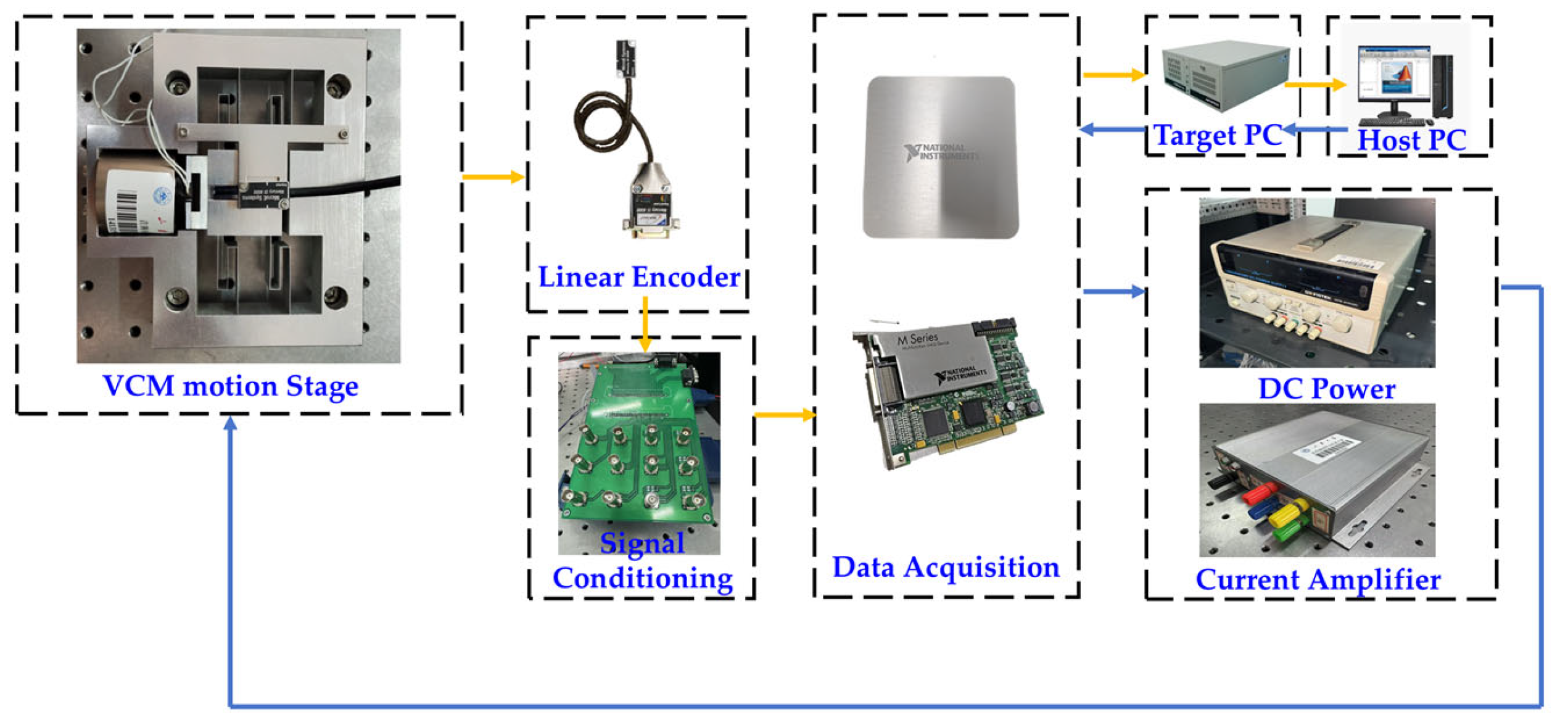
The hardware of the VCM motion system studied in this paper is shown in Figure 5. It mainly includes a DC power supply, a current amplifier, a signal acquisition module, a VCM driver, a flexure mechanism stage, and a grating linear encoder measurement module. The system implements motion control and data acquisition based on the xPC control platform. The user sets the excitation signal through the host computer, and the control command is sent to the target computer via a high-speed data bus. After signal conditioning and current amplification, the command drives the VCM. The grating scale detects the position in real time and feeds it back to the data acquisition card, which then sends it back to the host computer via the data bus, thereby obtaining the plant frequency-domain data online. Based on the collected frequency-domain data, offline controller optimization is performed on the host computer, and the optimized controller parameters are updated to the target computer for real-time online evaluation of control performance.

5.2. Frequency Response Data and Model Uncertainty

To account for plant variations under different operating conditions, 30 distinct frequency-response measurements ${\left\{{\mathrm{G}}_i\left(\mathrm{j}\mathsf{\omega }\right)\right\}}_{i=1}^{30}$ were experimentally collected. The frequency-response data were directly acquired using a frequency spectrum analyzer through swept-sine testing:

$$\mathrm{y} \left[\mathrm{k}\right] = \mathrm{Asin}\left(2\mathsf{\pi }\left({\mathrm{f}}_0\mathrm{k}{\mathrm{T}}_{\mathrm{s}}+{\displaystyle \frac{{\mathrm{f}}_1-{\mathrm{f}}_0}{2\mathrm{N}{\mathrm{T}}_{\mathrm{s}}}}{\left(\mathrm{k}{\mathrm{T}}_{\mathrm{s}}\right)}^2\right)\right),$$

(38)

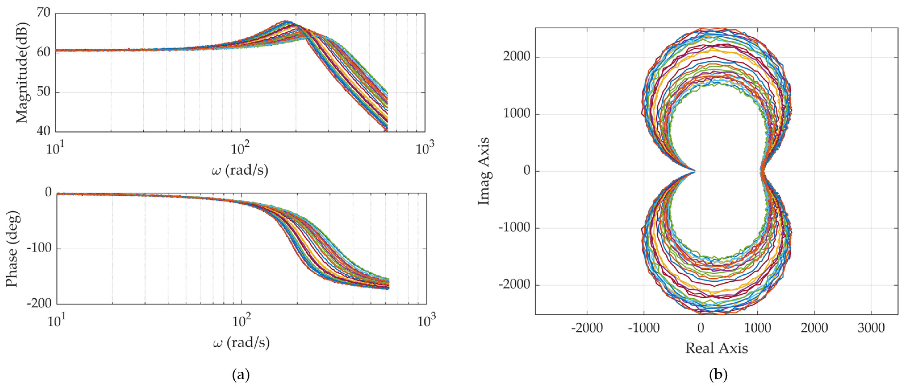
where A = 0.005~0.012, ${\mathrm{f}}_0 = 1 \mathrm{Hz}$, ${\mathrm{f}}_1 = 100 \mathrm{Hz}$, and ${\mathrm{T}}_{\mathrm{s}} = 50 \mathsf{\mu }\mathrm{s}$. The measured frequency responses were evaluated on a frequency grid consisting of 300 frequency samples. To capture operating-condition uncertainty, repeated identification experiments were conducted under different payload conditions, where the load mass varied from 0 g to 70 g. Consequently, the resulting datasets contain both plant variations and measurement variability under different operating conditions. All datasets were collected under normal laboratory conditions (approximately 25 °C), and potential temperature-induced variations, together with other operating-condition uncertainties, were inherently captured in the measured frequency-response data. Figure 6a shows the Bode diagrams of all 30 models, while Figure 6b presents the corresponding Nyquist plots. The spread among the responses reveals considerable model uncertainty, especially near the structural resonance around 20 Hz, motivating the use of a robust data-based design.

5.3. Selection of Laguerre Basis Order

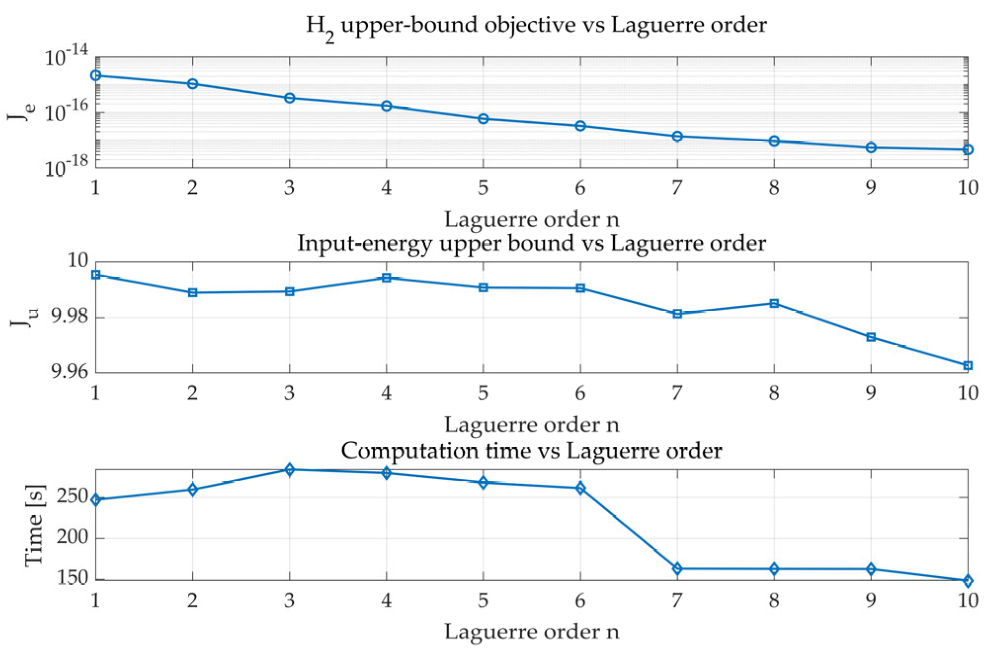
The Youla parameter Q′(z) was represented using Laguerre basis functions with an adjustable order n. Figure 7 shows that the H₂ upper-bound objective J_e is relatively sensitive to the Laguerre basis order n, especially in low-order cases, where increasing n significantly improves closed-loop performance. In contrast, the input-energy upper bound J_u is much less sensitive to change in basis order variation and remains nearly unchanged for all tested orders. Although higher basis orders can further reduce J_e, the improvement gradually saturates while controller complexity and implementation burden increase. Considering the trade-off among performance improvement, computational complexity, and the realizable controller order of the xPC real-time system, the Laguerre basis order was finally selected as n = 4.

5.4. Disturbance Estimation Performance of the Q′

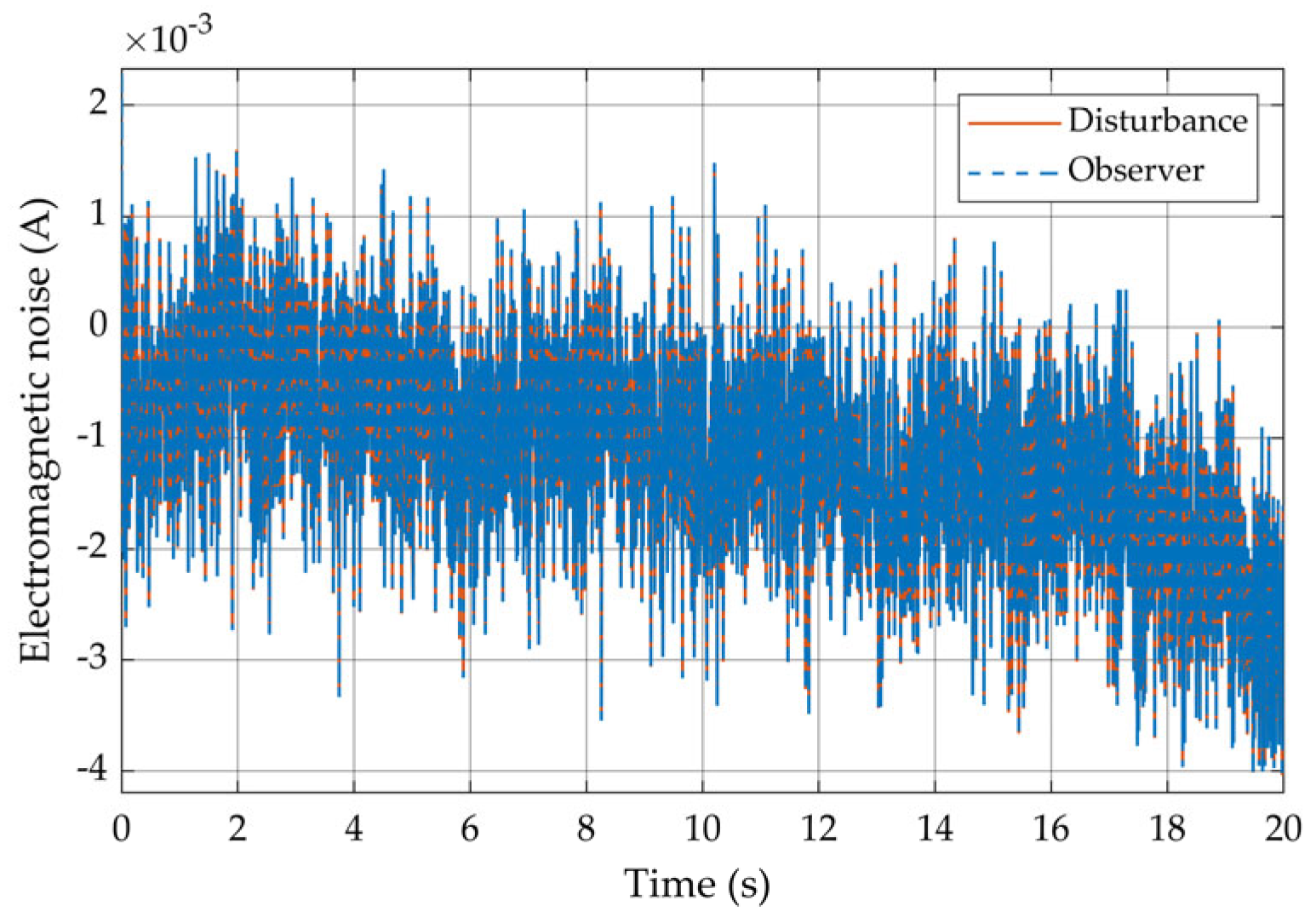
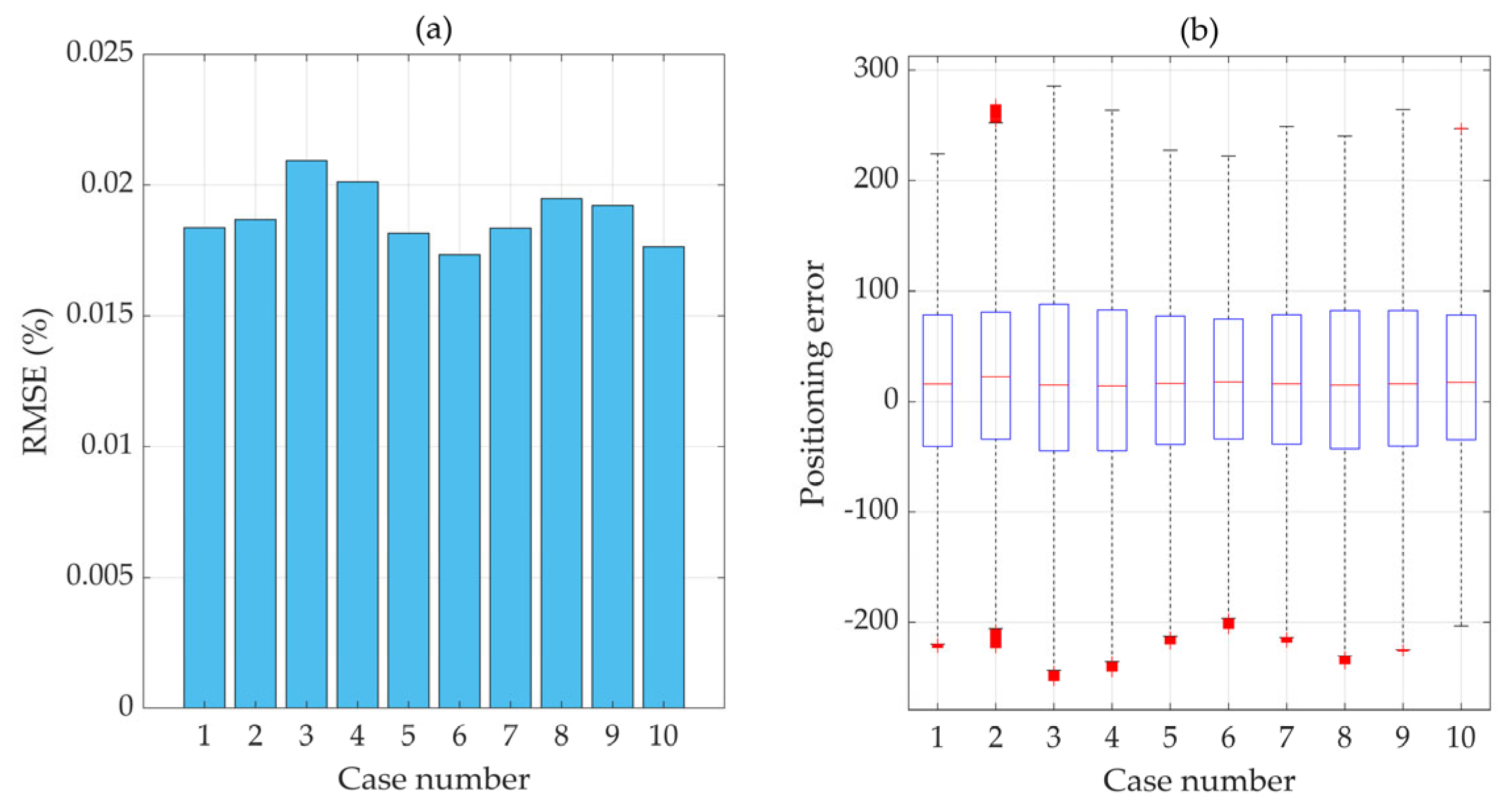
Following the steps outlined in Table 1, this section first fits the parameterized expression of the Q′, which is optimized for the VCM motion stage using a Laguerre basis, into a z-domain transfer function. The resulting expression is given in Equation (39). This filter is then used to observe the input noise of the VCM during data acquisition; Figure 8 presents the observed disturbance under an electromagnetic noise condition, where the average estimation error was 2.27 × 10⁻⁵. For robustness validation, ten datasets were randomly selected from the measured database as independent test cases. For each case, the steady-state tracking performance was evaluated using the normalized RMSE and maximum positioning error, as shown in Figure 9. Based on the statistics obtained from the ten validation experiments, 90% confidence intervals were computed using Student’s t-distribution. Results show an average RMSE of 0.0188% (90% CI: ±0.0006%) and an average maximum positioning error of 0.0499% (90% CI: ±0.0022%, all cases <0.05%). Thus, the controller maintains highly consistent positioning performance and strong robustness under varying operating conditions.

$$Q_{\prime }\left(\mathrm{z}\right)= 1 \times {10}^{-5} \times {\displaystyle \frac{1.467+2.88{\mathrm{z}}^{-1}-8.72{\mathrm{z}}^{-2 }+2.93{\mathrm{z}}^{-3}+1.44{\mathrm{z}}^{-4}}{1-3.96{\mathrm{z}}^{-1}+5.89{\mathrm{z}}^{-2}-3.891{\mathrm{z}}^{-3}+0.96{\mathrm{z}}^{-4}}}.$$

(39)

5.5. Tracking Performance Comparison Under Different Signals

To ensure a fair comparison, all baseline controllers were tuned under identical experimental conditions, including the same plant measurement data, sampling frequency, reference input, actuator limits, and performance metrics. Additionally, the controller bandwidth and transient response speed were adjusted to comparable levels, so that the comparison reflects differences in control structures rather than tuning artifacts. For ADRC, a bandwidth-parameterization method was used. The controller bandwidth was initially set to ${\mathsf{\omega }}_{\mathrm{c}} = 70$. The observer bandwidth ${\mathsf{\omega }}_0$ was chosen within $\left[{5\mathsf{\omega }}_{\mathrm{c}}, {10\mathsf{\omega }}_{\mathrm{c}}\right]$; ${\mathsf{\omega }}_0 = 700$ was finally selected. For the PID controller, the proportional and integral gains were optimized using a genetic algorithm within a loop-shaping framework consisting of a notch filter, a low-pass filter, and a reference prefilter. The objective function combined the ITAE criterion, settling time, overshoot, steady-state error, and response smoothness. The population size was set to 30, the maximum number of generations was 40, and the crossover probability was 0.8. In the proposed framework, the initial controller K₀ was designed as an H_∞ robust controller with weighting functions ${\mathrm{W}}_1 = {\displaystyle \frac{1.5}{\mathrm{s} + 0.001}}$ and ${\mathrm{W}}_2 = {\displaystyle \frac{0.7943 + 0.0036\mathrm{s} + 4.106 \times {10}^{-6}{\mathrm{s}}^2}{1 \times {10}^{-6}{\mathrm{s}}^2 + 0.002\mathrm{s} + 1}}$. The resulting H_∞ controller serves as the baseline stabilizing controller K₀, on which the proposed Youla-parameterized optimization is performed.

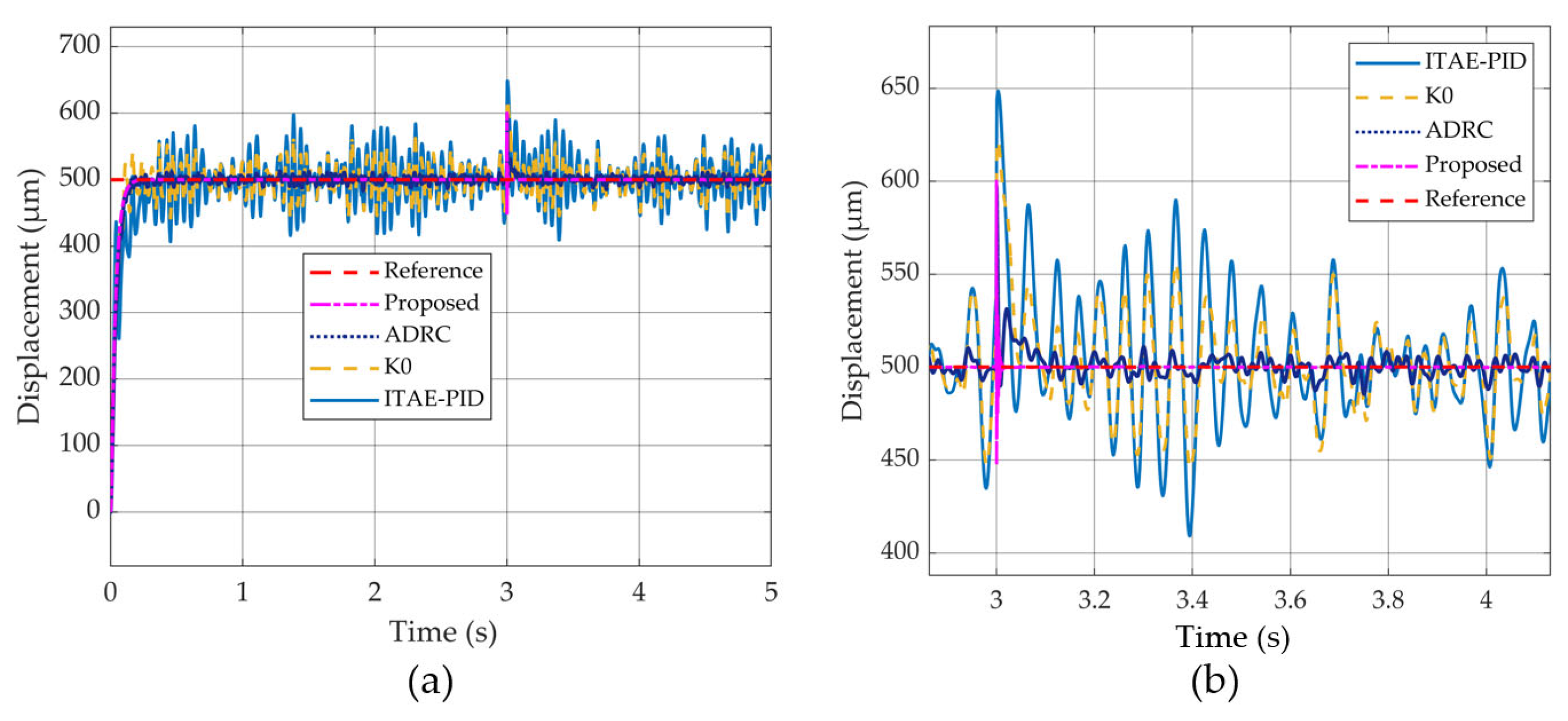
The VCM motion stage is required to perform large-stroke rapid approach motions, enabling efficient high-speed positioning. A step-response experiment was conducted to evaluate its performance, as illustrated in Figure 10a. With a reference input amplitude of 500 μm and a settling criterion within a 5% error band, the settling times of the ADRC, ITAE-PID, K0, and proposed controllers were measured as 0.29 s, 0.38 s, 0.25 s, and 0.22 s, respectively. To evaluate disturbance-rejection performance, a step disturbance with an amplitude of 100 μm was introduced at the 3 s mark during the step-response test shown in Figure 10b. Among the different methods, the proposed method exhibits the strongest disturbance-rejection capability, achieving rapid suppression within 0.013 s. The ADRC method ranks second and also provides good disturbance suppression, with a rejection time of about 0.17 s. K0 also achieves relatively fast suppression within 0.12 s, but it amplifies noise. The ITAE-PID controller exhibits the strongest noise amplification.

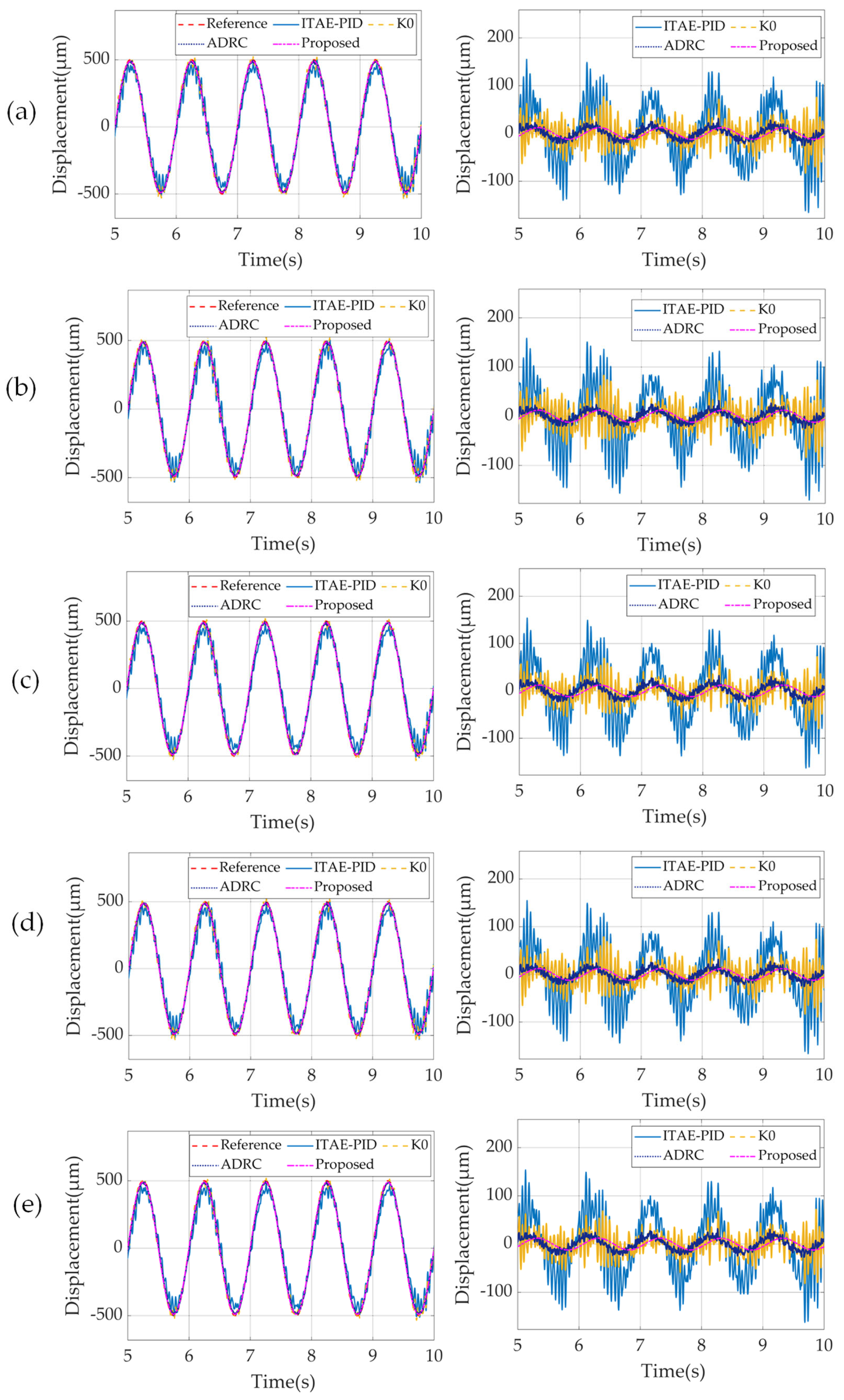
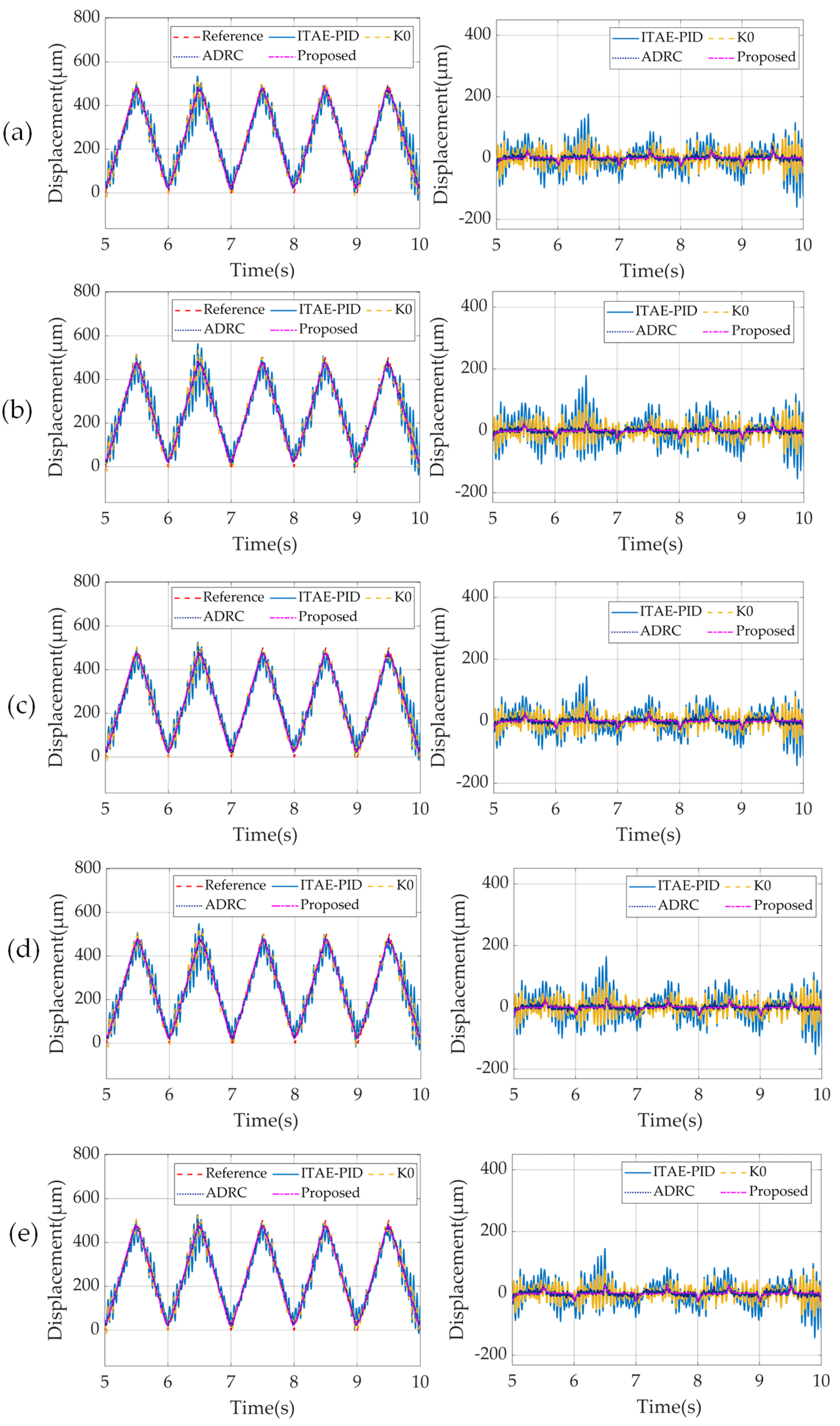
To better evaluate the positioning accuracy, dynamic response speed, and steady-state tracking capability under closed-loop control, tracking experiments were conducted using 1 Hz sinusoidal and triangular wave signals to assess the performance in following periodic continuous trajectories. The RMSE, mean RMSE, and corresponding standard deviations obtained from five repeated implementations were analyzed, and the experimental performance is presented in Figure 11 and Figure 12 and

Table 3. Comparison of RMSE values for the 1 Hz sinusoidal-signal-tracking response.

Controller	Test1 (%)	Test2 (%)	Test3 (%)	Test4 (%)	Test5 (%)	Mean ± Std (%)
ADRC	1.16	1.10	1.27	1.14	1.27	1.19 ± 0.081
ITAE-PID	6.05	6.19	6.30	6.12	6.30	6.19 ± 0.104
K0	2.55	2.71	2.41	2.58	2.41	2.53 ± 0.129
Proposed	0.87	0.87	0.87	0.87	0.87	0.87 ± 0.001

and

Table 4. Comparison of RMSE values for the 1 Hz triangular-signal-tracking response.

Controller	Test1 (%)	Test2 (%)	Test3 (%)	Test4 (%)	Test5 (%)	Mean ± Std (%)
ADRC	0.79	0.78	0.82	0.79	0.82	0.80 ± 0.022
ITAE-PID	4.25	4.69	4.09	4.41	4.09	4.31 ± 0.249
K0	2.49	2.61	2.34	2.51	2.34	2.46 ± 0.117
Proposed	0.59	0.59	0.59	0.59	0.59	0.59 ± 0.002

.

5.6. Robust Performance Comparison

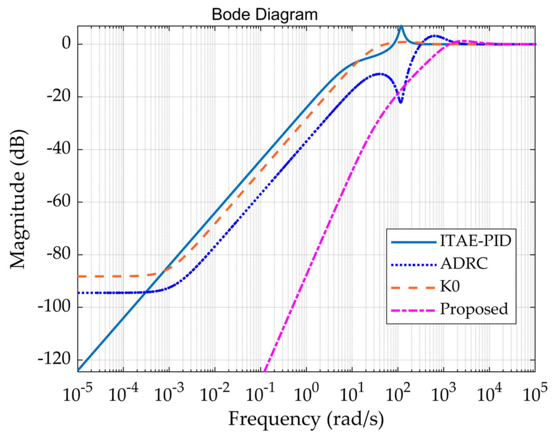
To verify the disturbance rejection capability and robustness of the proposed control strategy, the sensitivity function is analyzed in the frequency domain. Since the magnitude $\left|\mathrm{S}\left(\mathrm{j}\mathsf{\omega }\right)\right|$ directly reflects the system’s ability to suppress output disturbances, a smaller magnitude corresponds to better disturbance rejection and higher robustness.

As shown in Figure 13 and

Table 5. Comparison of frequency-domain indices.

Controller	Bandwidth (rad/s)	Peak Value (dB)	Resonant Amplitude (dB)
ADRC	248.66	3.18	−22.05
ITAE-PID	53.46	6.97	6.97
K0	24.79	0.86	0.82
Proposed	743.10	1.25	−17.36

, the ITAE-PID controller exhibits a resonance amplification peak of 6.97 dB near the dominant resonant frequency, indicating poor suppression of resonance-induced disturbances and limited robustness. In contrast, the ADRC achieves the strongest attenuation at the resonance peak, with a magnitude of −22.05 dB. The proposed controller provides the second-best resonance suppression performance, yielding a magnitude of −17.36 dB. Furthermore, the proposed controller demonstrates the strongest low-frequency disturbance attenuation and the highest closed-loop bandwidth among all compared methods. Its sensitivity peak is limited to only 1.25 dB, indicating that the bandwidth enhancement is achieved without sacrificing robustness. These results demonstrate that the proposed data-based Youla-Q controller achieves an effective balance among disturbance rejection, resonance suppression, and dynamic response performance.

6. Conclusions

This paper addressed the challenging problem of robust disturbance rejection for a VCM motion stage. The VCM system suffers from severe nonlinearities, unknown external disturbances and model parameter variations. Conventional DOBs rely heavily on an accurate plant model, which is difficult to obtain for such nonlinear and uncertain systems. To overcome this limitation, the present work developed a data-based robust DOB design that directly uses online measured input-output frequency-domain data of the VCM stage, thereby eliminating the need for an explicit mathematical model. The main contributions and findings are summarized as follows:

• Youla parameterization of the DOB structure. The standard DOB was reformulated within the Youla parameterization framework. Using the specific left-coprime factors, the equivalence between the Youla-parameterized controller and the standard DOB was rigorously established through algebraic derivations and block-diagram transformations. This transformation cast the DOB design into the selection of a stable Youla parameter $Q^{\prime }$, which directly corresponds to the $Q$-filter in the standard DOB.
• Multi-model robust stability and mixed $\mathrm{H}\infty /{\mathrm{H}}_2$ performance constraints. To capture the varying operating conditions, multiple frequency-response measurements ${\left\{{\mathrm{G}}_i\left(\mathrm{j}\mathsf{\omega }\right)\right\}}_{i=1}^L$ were collected. For the Youla-parameterized DOB, a convex robust stability condition and a convex H∞ performance constraint was established. Meanwhile, the H₂ tracking error energy and the control energy were expressed as convex quadratic functions via Parseval’s theorem. The Youla parameter $Q^{\prime }$ was then finitely parameterized using a Laguerre orthogonal basis. Consequently, all constraints and the objective became finite-dimensional convex functions of the basis coefficients. The complete implementation procedure was detailed in Table 1.
• Experimental validation. The proposed controller was compared with the ITAE-PID, ADRC, and baseline K₀ controllers, which possess comparable control capabilities. Comprehensive comparisons were conducted in terms of optimization result validation, disturbance rejection, tracking performance, and robustness. Step disturbance experiments demonstrated that the proposed method suppresses disturbances rapidly within 0.013 s. In addition, five repeated tracking experiments using 1 Hz sinusoidal and triangular reference signals were carried out. The results showed that the proposed controller achieves average RMSE values of 0.87% and 0.59%, respectively, which are lower than those of the ITAE-PID, ADRC, and K₀ controllers. Furthermore, sensitivity-function analysis of the closed-loop system reveals that the proposed method provides excellent low-frequency disturbance attenuation and achieves a higher closed-loop bandwidth while maintaining a relatively small waterbed effect. These results collectively verify the effectiveness of the proposed data-driven Youla-Q controller.

Future research will extend the approach to dual stage systems, develop online adaptive versions of the optimizer, and explore machine-learning techniques to further reduce conservatism.

References

1. Tonoy, A.A.R.; Ahmed, M.; Khan, M.R. Precision Mechanical Systems In Semiconductor Lithography Equipment Design And Development. Am. J. Adv. Technol. Eng. Solut. 2025, 1, 71–97. [Google Scholar] [CrossRef]
2. Fukada, S. Ultra-Precision One-Millimeter Stroke Flexure-Based Positioning Mechanism with Motion Control for Surface Topography Processing and Measurement Function. Int. J. Autom. Technol. 2025, 19, 405–424. [Google Scholar] [CrossRef]
3. Gao, X.; Deng, J.; Chang, Q.; Zhang, S.; Li, J.; Liu, J.; Liu, Y. Performance Investigation and Improvement of a Two-DOF Inertial Piezoelectric Robotic Insertion Device for Capillary Micropuncture. IEEE/ASME Trans. Mechatron. 2025, 30, 2189–2198. [Google Scholar] [CrossRef]
4. Zhang, L.; Zhang, P.; Jiang, B.; Yan, H. Research Trends in Methods for Controlling Macro-Micro Motion Platforms. Nanotechnol. Precis. Eng. 2023, 6, 035001. [Google Scholar] [CrossRef]
5. Kwon, S.; Chung, W.K. A Discrete-Time Design and Analysis of Perturbation Observer for Motion Control Applications. IEEE Trans. Control Syst. Technol. 2003, 11, 399–407. [Google Scholar] [CrossRef]
6. Zhang, W.; Yan, P.; Liu, P. Enhanced Piezo-Driven Compliant Motion Stage by Electromagnetically Tunable Mechanical Resonance. Int. J. Mech. Sci. 2025, 305, 110706. [Google Scholar] [CrossRef]
7. Zhang, X.; Zhang, X.; Xue, W.; Xin, B. An Overview on Recent Progress of Extended State Observers for Uncertain Systems: Methods, Theory, and Applications. Adv. Control Appl. 2021, 3, e89. [Google Scholar] [CrossRef]
8. Du, Y.; Cao, W.; She, J. Analysis and Design of Active Disturbance Rejection Control with an Improved Extended State Observer for Systems with Measurement Noise. IEEE Trans. Ind. Electron. 2023, 70, 855–865. [Google Scholar] [CrossRef]
9. Zhong, Q.-C.; Kuperman, A.; Stobart, R.K. Design of UDE-Based Controllers from Their Two-Degree-of-Freedom Nature. Int. J. Robust. Nonlinear Control 2011, 21, 1994–2008. [Google Scholar] [CrossRef]
10. Yang, C.; Wang, Y.; Youcef-Toumi, K. Hierarchical Antidisturbance Control of a Piezoelectric Stage via Combined Disturbance Observer and Error-Based ADRC. IEEE Trans. Ind. Electron. 2022, 69, 5060–5070. [Google Scholar] [CrossRef]
11. Naghdi, M.; Izadi, I. Fuzzy Extended State Observer for Robust Sliding Mode Control of Piezoelectric Actuators. IEEE Access 2024, 12, 43924–43931. [Google Scholar] [CrossRef]
12. Yue, J.; Liu, Z.; Su, H. Data-Driven Adaptive Extended State Observer-Based Model-Free Disturbance Rejection Control for DC–DC Converters. IEEE Trans. Ind. Electron. 2024, 71, 7745–7755. [Google Scholar] [CrossRef]
13. Li, X.; Chen, S.-L.; Teo, C.S.; Tan, K.K. Enhanced Sensitivity Shaping by Data-Based Tuning of Disturbance Observer with Non-Binomial Filter. ISA Trans. 2019, 85, 284–292. [Google Scholar] [CrossRef] [PubMed]
14. Liu, J.; Huang, T.; Tao, G.; Guo, K.; Li, D.; Cao, H. Modified Data-Driven Disturbance Observer with Its Application in Quadrant Glitch Compensation of Ball Screw Feed-Drive System. IEEE Trans. Ind. Electron. 2025, 72, 167–176. [Google Scholar] [CrossRef]
15. Zheng, M.; Lyu, X.; Liang, X.; Zhang, F. A Generalized Design Method for Learning-Based Disturbance Observer. IEEE/ASME Trans. Mechatron. 2021, 26, 45–54. [Google Scholar] [CrossRef]
16. Feng, W.; Zhang, Y.; Zhang, J. Generalized Internal Model Control of Voice Coil Actuator Fast Steering Mirror Under Parameter Perturbations. IEEE/ASME Trans. Mechatron. 2025, 30, 6164–6174. [Google Scholar] [CrossRef]
17. Xu, J.; Chen, X.; Tan, Y.; Zhou, K. Multiobjective Complementary Control. IEEE Trans. Autom. Control 2025, 70, 3556–3570. [Google Scholar] [CrossRef]
18. Xia, W.; Mao, Y.; Tang, M.; Zhang, B.; Liu, C. An Adaptive Error-Based Observer Method in Electro-Optical Tracking System. Measurement 2024, 232, 114638. [Google Scholar] [CrossRef]
19. Hu, X.; Laks, J.; Guo, G.; Chen, X. Iterative Youla-Kucera Loop Shaping For Precision Motion Control. IFAC-PapersOnLine 2025, 59, 575–580. [Google Scholar] [CrossRef]
20. Ding, B.; Zhao, J.; Li, Y. Design of a Spatial Constant-Force End-Effector for Polishing/Deburring Operations. Int. J. Adv. Manuf. Technol. 2021, 116, 3507–3515. [Google Scholar] [CrossRef]
21. Hedberg, E.; Löfberg, J.; Helmersson, A. A Pedagogical Path from the Internal Model Principle to Youla-Kučera Parametrization. IFAC-PapersOnLine 2020, 53, 17374–17379. [Google Scholar] [CrossRef]
22. Schuchert, P.; Gupta, V.; Karimi, A. Data-Driven Fixed-Structure Frequency-Based H 2 and H ∞ Controller Design. Automatica 2024, 160, 111398. [Google Scholar] [CrossRef]
23. Bagherieh, O. Estimation, Identification and Data-Driven Control Design for Hard Disk Drives, UC Berkeley, 2017. Available online: https://escholarship.org/uc/item/0998n097 (accessed on 15 June 2026).
24. Karimi, A.; Nicoletti, A.; Zhu, Y. Robust H Controller Design Using Frequency-domain Data via Convex Optimization. Int. J. Robust. Nonlinear 2018, 28, 3766–3783. [Google Scholar] [CrossRef]
25. Kjellqvist, O. Laguerre Bases for Youla-Parametrized Optimal-Controller Design: Numerical Issues and Solutions. Master’s Thesis, Lund University, Lund, Sweden, 2018. [Google Scholar]
Figure 1. Structure of the VCM motion stage.
Actuators 15 00355 g001
Figure 2. A general system with a standard DOB.
Actuators 15 00355 g002
Figure 3. Youla parameterization of controllers.
Actuators 15 00355 g003
Figure 4. The structure of DOB design using Youla parameterization.
Actuators 15 00355 g004
Figure 5. Experimental setup of the VCM motion system.
Actuators 15 00355 g005
Figure 6. Thirty sets of frequency-domain data collected under different operating conditions. (a) Bode plot. (b) Nyquist diagram.
Actuators 15 00355 g006
Figure 7. Sensitivity analysis of Laguerre basis order.
Actuators 15 00355 g007
Figure 8. Disturbance estimation.
Actuators 15 00355 g008
Figure 9. (a) RMSE distribution under ten operating scenarios. (b) Steady-state positioning error distribution.
Actuators 15 00355 g009
Figure 10. (a) Comparison of step-response experimental results. (b) Step disturbance performance comparison.
Actuators 15 00355 g010
Figure 11. 1 Hz sinusoidal-wave-tracking performance comparison. (a) Test 1; (b) Test 2; (c) Test 3; (d) Test 4; (e) Test 5.
Actuators 15 00355 g011
Figure 12. 1 Hz triangular-wave-tracking performance comparison. (a) Test 1; (b) Test 2; (c) Test 3; (d) Test 4; (e) Test 5.
Actuators 15 00355 g012
Figure 13. Comparison of magnitude characteristics of closed-loop sensitivity functions.
Actuators 15 00355 g013