Design of PI-P Controllers for a Class of Nonlinear Discrete Cascade Control Systems

Abstract

To address the parameter coordination and system integration issues in nonlinear discrete-time cascade control systems, this paper proposes, for the first time, a novel collaborative PI-P controller design method. First, an augmented state-space model for the PI-P controller is introduced, where the integral term is embedded into the state variables. Then, stability conditions are derived using Lyapunov stability theory, which are formulated as linear matrix inequality (LMI) constraints, enabling the simultaneous design of both primary and secondary controllers. The method is validated through simulations on a steam temperature control system. The results demonstrate that the proposed method outperforms conventional methods, achieving a faster response, reduced overshoot, and enhanced robustness. Moreover, the proposed method shows strong disturbance rejection capability and improved overall dynamic performance, further confirming its effectiveness and potential for application in nonlinear discrete-time cascade control systems.

1. Introduction

Cascade control employs a hierarchical strategy through coordinated primary and secondary loops. The primary controller maintains the core process variable to ensure final control accuracy, while the secondary controller rapidly suppresses local disturbances within the main loop, significantly improving the system’s disturbance rejection capability [1,2]. This control method has gained widespread adoption in critical industrial applications due to its superior performance. It plays essential roles in precise temperature control in thermal power plants [3], stable tank level maintenance and flow control in chemical processes [4,5], dynamic regulation of key parameters in power systems [6], pressure control in petrochemical reactors, heat exchanger temperature management, and metallurgical process temperature control. By leveraging the synergy between primary and secondary control loops, this approach not only ensures continuous stable operation of complex industrial processes but also delivers enhanced control precision, making it a fundamental enabling technology for modern industrial production [3,7].

As industrial automation shifts toward digitalization and intelligence, cascade control systems are increasingly characterized by the superposition of nonlinearity and discretization [8,9,10]. Nonlinear factors such as material coupling and reaction kinetics in industrial processes interact with discrete sampling, resulting in increasingly complex system dynamics [11,12,13]. This complexity poses significant challenges to cascade control: traditional linearized modeling methods struggle to accurately capture the essential characteristics of nonlinear components and fail to quantify the coupling effects between nonlinearity and discretization. Furthermore, the introduction of integral action to meet industrial requirements for steady-state error control further exacerbates the difficulties in system modeling and stability analysis [14,15]. Consequently, traditional cascade control strategies in nonlinear scenarios often exhibit excessive overshoot and response lag, failing to meet the control demands of complex industrial systems [16,17,18]. By focusing on the superimposed effects of nonlinearity and discretization, this analysis highlights their adverse impacts on cascade control modeling, stability, and performance, thereby exposing the inadequacy of traditional cascade control in nonlinear applications.

Cascade control is inherently a complex multi-loop closed-loop system that shares connections with but differs significantly from single-loop systems [19,20]. A single-loop system employs only one controller and one measurement point to form a feedback loop, offering structural simplicity and ease of implementation [21,22]. However, it can only regulate global disturbances and exhibits limited capability in suppressing local disturbances [23,24]. In contrast, cascade control embeds a secondary loop within the primary loop, enabling localized disturbances—which are challenging to handle in a single-loop structure—to be rapidly compensated within the secondary loop. This allows the primary loop to focus solely on the core control objective, substantially enhancing the system’s ability to handle complex disturbances [1,3]. For instance, in main steam temperature control in thermal power plants [25,26], the secondary loop of a cascade system quickly suppresses fluctuations in desuperheating water flow, while the primary loop maintains stable steam temperature. Compared to a single-loop system, this results in accelerated disturbance rejection and significantly improved control accuracy [26,27]. By comparing cascade control with single-loop architectures, the advantage of enhanced local disturbance suppression through the secondary loop is emphasized, highlighting the superiority of cascade control in complex closed-loop scenarios.

Existing cascade controller design methods can generally be classified into three categories. The first category relies on empirical or industrial tuning rules, which are simple to implement but often fail to guarantee closed-loop stability and coordinated optimization of primary and secondary loops. The second category employs intelligent optimization algorithms or nonlinear optimization techniques to simultaneously tune cascade controller parameters. Although satisfactory control performance can be achieved, the computational burden is often high and theoretical stability guarantees are generally difficult to establish. The third category is based on state-space and modern control theory, where controller parameters are determined through analytical design procedures. Compared with these approaches, the method proposed in this paper formulates the coordinated PI-P controller design problem for nonlinear discrete cascade systems within a unified state-space framework and transforms the controller synthesis conditions into solvable LMI constraints, thereby enabling simultaneous parameter tuning together with theoretical stability guarantees.

Recent studies have also investigated simultaneous tuning of cascade controllers through nonlinear optimization techniques [28]. For example, Torga et al. proposed a coordinated tuning framework based on nonlinear optimization. However, the obtained controller parameters are determined through iterative numerical optimization, whereas the present work focuses on a state-space-based nonlinear PI-P controller design with Lyapunov stability guarantees. In response to the aforementioned requirements for handling nonlinearity, discretization effects, and closed-loop control, the combined scheme of a PI controller in the primary loop and a P controller in the secondary loop demonstrates clear rationale. From a control performance perspective, the primary loop must satisfy both dynamic response speed and steady-state accuracy. The proportional component of the PI controller accelerates response, while the integral action eliminates steady-state error [14,15], aligning with the core control objectives. The secondary loop is primarily tasked with rapid suppression of localized disturbances [29]; it achieves fast response without requiring integral action, and the simple structure and low computational load of the P controller meet the millisecond-level real-time control demands [30,31]. From a technical adaptability standpoint, traditional cascade tuning often relies on empirical methods that fail to coordinate the primary and secondary loops effectively [32,33]. In contrast, the PI-P combination enables integrated parameter optimization, avoiding the high computational complexity and limited real-time applicability of intelligent optimization algorithms [19,26]. Moreover, this scheme is compatible with industrial discrete control architectures such as PLC and DCS [34,35], ensuring feasibility for practical implementation. By addressing both control requirements and technical adaptability, this analysis clarifies the selection rationale for the PI + P cascade structure, highlights the functional strengths and engineering suitability of the PI-P controllers, and demonstrates the scheme’s applicability to nonlinear and discretized industrial scenarios.

To overcome the limitations of existing cascade control in nonlinear discrete systems, this paper proposes three core innovations that collectively form a complete and practically viable technical solution:

1.

Extended state-space modeling for nonlinear cascade systems. An augmented state-space framework is developed by embedding integral terms directly into the state variables, allowing unified representation of nonlinear elements and integral dynamics. Unlike traditional transfer function-based or single-loop LMI PI/PID designs, this approach explicitly captures coupling effects between primary and secondary loops, providing a solid theoretical basis for coordinated controller parameter synthesis.

2.

Lyapunov-based stability analysis and coordinated PI-P tuning framework. A Lyapunov functional with embedded nonlinear compensation is constructed, and sector-bounded constraints are employed to reformulate the stability conditions as convex LMIs. This allows integrated parameter optimization of PI-P controllers in a theoretically supported manner, distinguishing it from conventional empirical tuning or single-loop LMI designs. The method provides reproducible and systematic parameter selection that accounts for loop interactions and nonlinearities.

3.

A complete simulation-validated framework for industrial applicability. The proposed methodology integrates theoretical modeling, simulation verification, and practical adaptation. Its effectiveness is demonstrated on a main steam temperature control system, showing coordinated suppression of coupled disturbances. Unlike previous LMI or empirical methods that primarily target nominal single-loop systems, the framework can be applied directly to industrial discrete control processes, such as chemical or metallurgical plants, without extensive modification, thus providing a systematic and practical design tool.

The structure of this paper is organized as follows. Section 2 establishes a nonlinear CCS model with a PI controller as the primary controller and a P controller as the secondary controller. Section 3 derives sufficient conditions for the stability of the nonlinear CCS and proposes a co-design method for the primary and secondary controllers based on these conditions. Section 4 presents a simulation case of main steam temperature cascade control with the PI-P control structure to validate the effectiveness and feasibility of the proposed method. Section 5 provides the conclusion of this paper.

Notation 1.

Let I denote the identity matrix of appropriate dimensions. For a matrix $X\in R^{n\times n}$, $X>0$ (respectively, $X<0$) indicates that X is a real symmetric positive definite (respectively, negative definite) matrix.

2. Nonlinear CCS Modeling

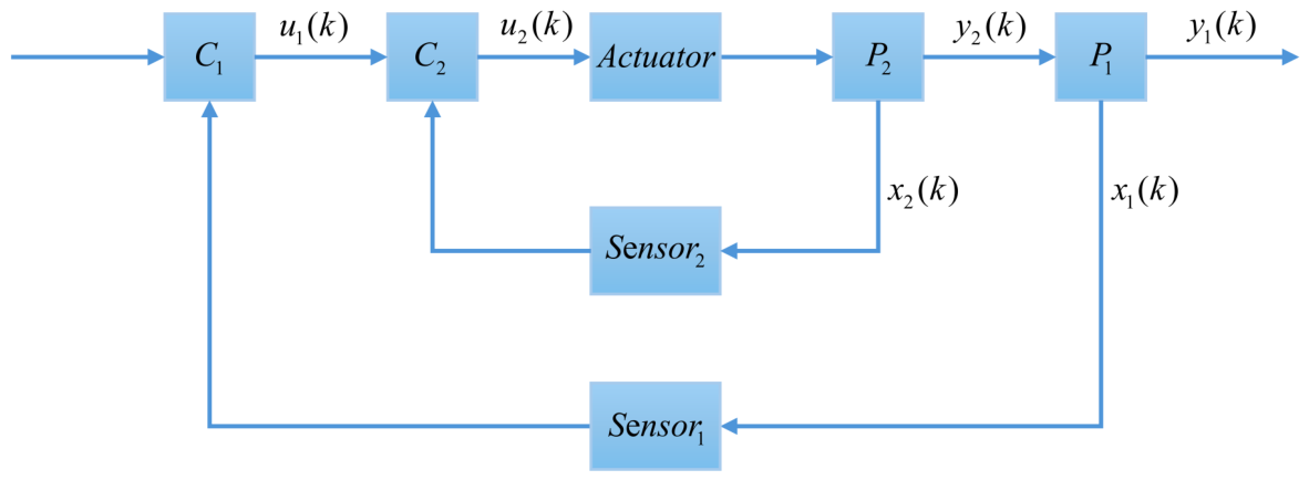
This section establishes a general model of “Primary loop PI and Secondary loop P” under the nonlinear discrete cascade control framework shown in Figure 1. In the figure, $P_1$ represents the primary controlled object, $C_1$ is the primary discrete PI controller, $S_1$ is the primary sensor responsible for sampling the primary object state $x_1\left(k\right)$ and sending it to $C_1$; $P_2$ denotes the secondary controlled object, $C_2$ is the discrete P controller, $S_2$ is the secondary sensor feeding back the secondary object state $x_2\left(k\right)$ to $C_2$; the actuator A is placed between $C_2$ and $P_2$, its output directly drives the secondary controlled object. The output of the secondary controlled object $y_2\left(k\right)$ serves as the input to the primary controlled object, forming cascade coupling. Within the discrete-time framework, the main controller’s integration mechanism and the auxiliary P controller’s swift regulation establish dynamical coordination, forming a unified basis for subsequent stability verification and parameter design.

The primary controlled object can be described as:

$$\left\{\begin{array}{c}{\dot{x}}_1\left(t\right)=A_1{x}_1\left(t\right)+B_1{y}_2\left(t\right)\hfill \\ y_1\left(t\right)=C_1{x}_1\left(t\right)\hfill \end{array}\right.$$

(1)

where $x_1\left(t\right)\in R^n$ is the state vector of the primary controlled object, $y_2\left(t\right)$ is its input, which is also the input of the primary controlled object. $A_1,B_1,C_1$ are constant matrices of appropriate dimensions.

The secondary controlled object is nonlinear and can be described as:

$$\left\{\begin{array}{c}{\dot{x}}_2\left(t\right)=f(x_1\left(t\right),x_2\left(t\right))\hfill \\ y_2\left(t\right)=C_2{x}_2\left(t\right)\hfill \end{array}\right.$$

(2)

$f(x_1\left(t\right),x_2\left(t\right))$ satisfies the Lurie system, thus it can be represented as a linear part and a nonlinear part. Therefore, the secondary controlled object can be expressed as:

$$\left\{\begin{array}{c}{\dot{x}}_2\left(t\right)=A_2{x}_2\left(t\right)+B_2{u}_2\left(t\right)+B_{3}w\left(t\right)\hfill \\ y_2\left(t\right)=C_2{x}_2\left(t\right)\hfill \end{array}\right.$$

(3)

where $x_2\left(t\right)\in R^n$ is the state vector of the secondary system, $u_2\left(t\right)\in R^m$ is the input of the secondary system, $y_2\left(t\right)$ is the output of the secondary system. $A_2,B_2,B_3,C_2$ are constant matrices of appropriate dimensions. The nonlinear part $w\left(t\right)$ can be denoted as $-\Phi (t,y_1\left(t\right))$. $\Phi (t,y_1\left(t\right))$ is piecewise-continuous in t and satisfies the local Lipschitz condition on $y_1\left(t\right)$, and $\Phi (t,0)=0$, then for $t\ge 0$ and $y_1\left(t\right)$, it satisfies the following condition:

$${\left[\Phi (t,y_1\left(t\right))-N_1{y}_1\left(t\right)\right]}^T\left[\Phi (t,y_1\left(t\right))-N_2{y}_1\left(t\right)\right]\le 0$$

where $N_2-N_1>0$, meaning the nonlinear function satisfies the sector condition $\left[N_1,N_2\right]$. Let $N=N_2-N_1$, then a special sector constraint condition for the nonlinear function can be obtained:

$${\Phi }^T(t,y_1\left(t\right))\left[\Phi (t,y_1\left(t\right))-N{y}_1\left(t\right)\right]\le 0$$

Remark 1.

The nonlinear term $\Phi (t,y_1\left(t\right))$ represents the effects of unmodeled dynamics, parameter variations, and nonlinear coupling in the cascade control system. It is modeled using a Lurie system and assumed to satisfy a sector-bounded condition defined by $N_1$ and $N_2$, which provides a bounded description of the nonlinearity and allows it to be incorporated into the Lyapunov-based stability analysis and LMI design. For the considered case, a conservative choice $N_1=0$ and $N_2=I$ is adopted, yielding $N=N_2-N_1=I$. The matrix $B_3$ describes how the nonlinear term enters the state-space model and affects each state variable, reflecting the structural characteristics of the original system.

Discretization of (1) and (2) across the interval $\left[kh,(k+1)h\right]$ leads to:

$$\left\{\begin{array}{c}{x}_1(k+1)={\Phi }_1{x}_1\left(k\right)+{\Gamma }_1{y}_2\left(k\right)\hfill \\ y_1\left(k\right)=C_1{x}_1\left(k\right)\hfill \end{array}\right.$$

(4)

where ${\Phi }_1=e^{A_{1}h}$, ${\Gamma }_1={\int }_0^h{e}^{A_{1}s}ds{B}_1$, and

$$\left\{\begin{array}{c}{x}_2(k+1)={\Phi }_2{x}_2\left(k\right)+{\Gamma }_2{u}_2\left(k\right)+{\Psi }_{3}w\left(k\right)\hfill \\ y_2\left(k\right)=C_2{x}_2\left(k\right)\hfill \end{array}\right.$$

(5)

where ${\Phi }_2=e^{A_{2}h}$, ${\Gamma }_2={\int }_0^h{e}^{A_{2}s}ds{B}_2$, ${\Psi }_3={\int }_0^h{e}^{A_{2}s}ds{B}_3$.

Remark 2.

The nonlinear cascade control system is modeled by (4) and (5). The cascade control system features a dual closed-loop structure with two controllers connected in series. The primary design objective focuses on enhancing main variable control through the incorporation of an auxiliary control loop. The secondary loop possesses fast regulation characteristics, enabling it to quickly suppress disturbances entering it, while also exhibiting certain robustness. These features work together to effectively optimize the dynamic performance of the nonlinear controlled object.

Remark 3.

Considering the challenges posed by nonlinear systems, few studies have described the closed-loop state-space model for a “PI controller with state feedback” even in nonlinear single-loop systems, and achieving one-step optimal PI tuning remains largely unexplored. Given this methodological gap, our work does not directly extend such approaches to cascade systems. Instead, we derive a closed-loop state-space model for a nonlinear cascade system incorporating a PI controller and establish corresponding design conditions that account for nonlinear characteristics. This approach enables simultaneous quantitative optimization of dynamic performance and robustness for both loops under nonlinear effects.

Remark 4.

The secondary controller is a state feedback controller, satisfying the state feedback expression $u\left(t\right)=kx\left(t\right)+v\left(t\right)$, where $v\left(t\right)$ is the reference input, that is, the set value. For convenience in calculating, let $v\left(t\right)=0$. The primary controller $u_1\left(t\right)$ is also a state feedback controller with a reference input of 0.

While single-loop systems commonly utilize P, PI, and PID controllers, nonlinear CCS implementations remain predominantly based on P control with state feedback. To further enhance control performance, this paper proposes modifying the main loop controller to a PI structure and introducing an integration interval $\tau$. The control law of the main PI controller under this configuration is given by:

$$u_1\left(t\right)=K_p{x}_1\left(t\right)+K_i{\int }_{t-\tau }^t{x}_1\left(t\right)dt$$

(6)

The discretized form can be obtained as follows:

$$\begin{array}{cc}\hfill u_1\left(k\right)& =K_p{x}_1\left(k\right)+K_{i}h{\displaystyle \sum _{m=k-n-1}^{k-1}}{x}_1\left(m\right)\hfill \\ \hfill & =(K_p+K_{i}h)x_1\left(k\right)+K_{i}h{\displaystyle \sum _{m=k-n-1}^{k-1}}{x}_1\left(m\right)\hfill \end{array}$$

(7)

where $K_p$, $K_i$ are the proportional and integral gains to be designed, with h and n representing the sampling period and a settable constant, respectively.

A conventional discrete P controller is employed for the secondary loop, generating an output formed by two components: one is the output signal from the main controller, and the other is the state feedback signal of the secondary system. The output of this controller can be expressed as:

$$\begin{array}{cc}\hfill u_2\left(k\right)& =u_1\left(k\right)+K_2{x}_2\left(k\right)\hfill \\ \hfill & =(K_p+K_{i}h)x_1\left(k\right)\hfill \\ \hfill & +K_{i}h{\displaystyle \sum _{m=k-n-1}^{k-1}}{x}_1\left(m\right)+K_2{x}_2\left(k\right)\hfill \end{array}$$

(8)

The continuous-time nonlinear term $w\left(t\right)$ is discretized by sampling its instantaneous value at each sampling instant and representing it with the discrete-time index k, resulting in the corresponding discrete signal $w\left(k\right)$.

Under the assumption of complete state observability, the following closed-loop discrete nonlinear CCS model is constructed based on (4), (5), (7) and (8):

$$\left\{\begin{array}{c}{x}_1(k+1)={\Phi }_1{x}_1\left(k\right)+{\Gamma }_1{C}_2{x}_2\left(k\right)\hfill \\ x_2(k+1)={\Phi }_2{x}_2\left(k\right)+{\Gamma }_2{u}_2\left(k\right)+{\Psi }_{3}w\left(k\right)\hfill \\ y_1\left(k\right)=C_1{x}_1\left(k\right)\hfill \\ u_1\left(k\right)=(K_p+K_{i}h)x_1\left(k\right)+K_{i}h{\displaystyle {\sum }_{m=k-n-1}^{k-1}}{x}_1\left(m\right)\hfill \\ u_2\left(k\right)=u_1\left(k\right)+K_2{x}_2\left(k\right)\hfill \end{array}\right.$$

(9)

It should be emphasized that the proposed framework is developed for a class of nonlinear systems with sector-bounded nonlinearities.

Based on the established nonlinear system model (9), this paper constructs a nonlinear cascade control system based on the state-space method. This control system adopts a structure combining the primary loop PI control and the secondary loop P control to achieve dual-loop cooperative operation. For this nonlinear closed-loop system, this paper conducts a rigorous stability analysis using Lyapunov stability theory, effectively verifying the system’s closed-loop performance. The research results provide a theoretical basis for the further design and optimization of the controller.

Remark 5.

The primary controller’s integral signal in the developed model is composed of past state values covering the last $n+1$ sampling instants. The integral term is synthesized from the state sequence defined by time instances $k-1,k-2,\dots ,k-n-1$.

Remark 6.

For theoretical analysis, the reference input is assumed to be zero without loss of generality. This is achieved by defining the tracking error as the new system state and shifting the equilibrium point to the origin. Therefore, the subsequent stability analysis is conducted on the error system, and the obtained results remain applicable to nonzero reference inputs.

Remark 7.

For theoretical analysis, all system states are assumed to be available. This assumption is commonly adopted in cascade control design and facilitates the coordinated synthesis of controller parameters. In practical industrial systems, key process variables can often be measured directly, while unmeasurable states may be estimated using state observers. Therefore, the proposed framework can be extended to observer-based output feedback designs, which will be investigated in future work.

3. Stability of Nonlinear CCS

The primary objective of this section is to formulate sufficient conditions, based on the derived nonlinear cascade system (9), that guarantee asymptotic stability.

Theorem 1.

Given the primary controller parameters $K_p$, $K_i$, and the secondary controller gain $K_2$, if there exist positive definite matrices $P>0$, $Q_m>0$, $T>0$, $m\in \left[1,n+1\right]$, satisfying the matrix in (10), then the closed-loop system (9) is asymptotically stable.

$$\tilde{\Omega }=\left[\begin{array}{ccc}{\tilde{\Omega }}_{11}& {\tilde{\Omega }}_{12}& {\tilde{\Omega }}_{13}\\ *& -P& 0\\ *& *& -T\end{array}\right]<0$$

(10)

where

$${\tilde{\Omega }}_{11}=\left[\begin{array}{cccc}{\tilde{\theta }}_{11}& 0& 0& {\tilde{\theta }}_{14}\\ *& {\tilde{\theta }}_{22}& 0& 0\\ *& *& {\tilde{\theta }}_{33}& 0\\ *& *& *& {\tilde{\theta }}_{44}\end{array}\right],{\tilde{\theta }}_{11}=-P+{\displaystyle \sum _{m=1}^{n+1}}{Q}_m,$$

$${\tilde{\theta }}_{22}=-\mathrm{diag}[Q_1,Q_2,\dots ,Q_{n+1}],{\tilde{\theta }}_{14}=-C_1^T{N}^T$$

$${\tilde{\theta }}_{33}=-T,{\tilde{\theta }}_{44}=-I,{\tilde{\Omega }}_{12}={[P^T{\Phi }_1,\underset{n+1}{\underbrace{0,\dots ,0}},P^T\left({\Gamma }_1{C}_2\right),0]}^T,$$

$${\tilde{\Omega }}_{13}={[T^T{\Gamma }_2(K_p+K_{i}h),\underset{n+1}{\underbrace{h{T}^T\left({\Gamma }_2{K}_i\right),\dots ,h{T}^T\left({\Gamma }_2{K}_i\right)}},T^T({\Phi }_2+{\Gamma }_2{K}_2),T^T{\Psi }_3]}^T.$$

Proof. 

Consider the following Lyapunov function candidate $V\left(k\right)$, constructed with positive definite matrix $P>0$, $Q_m>0$, $T>0$, and $m\in \left[1,n+1\right]$.

$$V\left(k\right)=V_1\left(k\right)+V_2\left(k\right)+V_3\left(k\right)$$

(11)

where

$$\begin{array}{cc}\hfill & V_1\left(k\right)=x_1^T\left(k\right)P{x}_1\left(k\right),\hfill \\ \hfill & V_2\left(k\right)={\displaystyle \sum _{m=1}^{n+1}}{\displaystyle \sum _{s=k-m}^{k-1}}{x_1}^T\left(s\right)Q_m{x}_1\left(s\right),\hfill \\ \hfill & V_3\left(k\right)=x_2^T\left(k\right)T{x}_2\left(k\right),\hfill \end{array}$$

$$\begin{array}{cc}\hfill \Delta V\left(k\right)& =\Delta V_1\left(k\right)+\Delta V_2\left(k\right)+\Delta V_3\left(k\right)\hfill \end{array}$$

(12)

where

$$\begin{array}{cc}\hfill \Delta V_1\left(k\right)& =V_1(k+1)-V_1\left(k\right)\hfill \\ \hfill & =x_1^T(k+1)P{x}_1(k+1)-x_1^T\left(k\right)P{x}_1\left(k\right)\hfill \\ \hfill & =x_1^T\left(k\right){\Phi }_1^{T}P{\Phi }_1{x}_1\left(k\right)+2x_1^T\left(k\right){\Phi }_1^{T}P{\Gamma }_1{C}_2{x}_2\left(k\right)\hfill \\ \hfill & +x_2^T\left(k\right)C_2^T{\Gamma }_1^{T}P{\Gamma }_1{C}_2{x}_2\left(k\right)-x_1^T\left(k\right)P{x}_1\left(k\right)\hfill \\ \hfill & =x_1^T\left(k\right)\left[{\Phi }_1^{T}P{\Phi }_1-P\right]x_1\left(k\right)+2x_1^T\left(k\right){\Phi }_1^{T}P{\Gamma }_1{C}_2{x}_2\left(k\right)\hfill \\ \hfill & +x_2^T\left(k\right)C_2^T{\Gamma }_1^{T}P{\Gamma }_1{C}_2{x}_2\left(k\right),\hfill \\ \hfill \Delta V_2\left(k\right)& =V_2(k+1)-V_2\left(k\right)\hfill \\ \hfill & ={\displaystyle \sum _{m=1}^{n+1}}{\displaystyle \sum _{s=k+1-m}^k}{x}_1^T\left(s\right)Q_m{x}_1\left(s\right)-{\displaystyle \sum _{m=1}^{n+1}}{\displaystyle \sum _{s=k-m}^{k-1}}{x}_1^T\left(s\right)Q_m{x}_1\left(s\right)\hfill \\ \hfill & ={\displaystyle \sum _{m=1}^{n+1}}[x_1^T\left(k\right)Q_m{x}_1\left(k\right)+{\displaystyle \sum _{s=k+1-m}^{k-1}}{x}_1^T\left(s\right)Q_m{x}_1\left(s\right)]\hfill \\ \hfill & -{\displaystyle \sum _{m=1}^{n+1}}{\displaystyle \sum _{s=k-m}^{k-1}}{x}_1^T\left(s\right)Q_m{x}_1\left(s\right)\hfill \\ \hfill & ={\displaystyle \sum _{m=1}^{n+1}}{x}_1^T\left(k\right)Q_m{x}_1\left(k\right)-{\displaystyle \sum _{m=1}^{n+1}}{x}_1^T(k-m)Q_m{x}_1(k-m),\hfill \\ \hfill \Delta V_3\left(k\right)& =V_3(k+1)-V_3\left(k\right)\hfill \\ \hfill & =[({\Phi }_2+{\Gamma }_2{K}_2)x_2\left(k\right)+{\Gamma }_2(K_p+K_{i}h)x_1\left(k\right)+{\Gamma }_2{K}_{i}h{\displaystyle \sum _{m=k-n-1}^{k-1}}{x}_1\left(m\right)\hfill \\ \hfill & +{\Psi }_{3}w\left(k\right){]}^{T}T[({\Phi }_2+{\Gamma }_2{K}_2)x_2\left(k\right)+{\Gamma }_2(K_p+K_{i}h)x_1\left(k\right)\hfill \\ \hfill & +{\Gamma }_2{K}_{i}h{\displaystyle \sum _{m=k-n-1}^{k-1}}{x}_1\left(m\right)+{\Psi }_{3}w\left(k\right)]-x_2^T\left(k\right)T{x}_2\left(k\right)\hfill \\ \hfill & =x_2^T\left(k\right){({\Phi }_2+{\Gamma }_2{K}_2)}^{T}T({\Phi }_2+{\Gamma }_2{K}_2)x_2\left(k\right)\hfill \\ \hfill & +x_1^T\left(k\right){(K_p+K_{i}h)}^T{\Gamma }_2^{T}T{\Gamma }_2(K_p+K_{i}h)x_1\left(k\right)\hfill \\ \hfill & +{[{\displaystyle \sum _{m=k-n-1}^{k-1}}{x}_1\left(m\right)]}^T{\left({\Gamma }_2{K}_i\right)}^T{h}^{2}T{\Gamma }_2{K}_i{\displaystyle \sum _{m=k-n-1}^{k-1}}{x}_1\left(m\right)\hfill \\ \hfill & +w^T\left(k\right){\Psi }_3^{T}T{\Psi }_{3}w\left(k\right)+2x_1^T\left(k\right){(K_p+K_{i}h)}^T{\Gamma }_2^{T}T({\Phi }_2+{\Gamma }_2{K}_2)x_2\left(k\right)\hfill \\ \hfill & +2{[{\displaystyle \sum _{m=k-n-1}^{k-1}}{x}_1\left(m\right)]}^T{\left({\Gamma }_2{K}_i\right)}^{T}hT({\Phi }_2+{\Gamma }_2{K}_2)x_2\left(k\right)\hfill \\ \hfill & +2x_1^T\left(k\right){(K_p+K_{i}h)}^T{\Gamma }_2^{T}T{\Gamma }_2{K}_{i}h{\displaystyle \sum _{m=k-n-1}^{k-1}}{x}_1\left(m\right)\hfill \\ \hfill & +2x_1^T\left(k\right){(K_p+K_{i}h)}^T{\Gamma }_2^{T}T{\Psi }_{3}w\left(k\right)\hfill \\ \hfill & +2{[{\displaystyle \sum _{m=k-n-1}^{k-1}}{x}_1\left(m\right)]}^T{\left({\Gamma }_2{K}_i\right)}^{T}hT{\Psi }_{3}w\left(k\right)\hfill \\ \hfill & +2x_2^T\left(k\right){({\Phi }_2+{\Gamma }_2{K}_2)}^{T}T{\Psi }_{3}w\left(k\right)-x_2^T\left(k\right)T{x}_2\left(k\right)\hfill \end{array}$$

Combining the Lyapunov functionals obtained from the above calculations yields:

$$\begin{array}{cc}\hfill \Delta V\left(k\right)& \le \Delta V_1\left(k\right)+\Delta V_2\left(k\right)+\Delta V_3\left(k\right)-x_1\left(k\right)C_1^T{N}^{T}w\left(k\right)-w^T\left(k\right)w\left(k\right)\hfill \\ \hfill & \le {\xi }^T\left(k\right)\Omega \xi \left(k\right)\hfill \end{array}$$

(13)

where

$$\begin{array}{c}\hfill {\xi }^T\left(k\right)=[x_1^T\left(k\right),x_1^T(k-1),x_1^T(k-2),\cdots ,x_1^T(k-n-1),x_2^T\left(k\right),w^T\left(k\right)],\end{array}$$

and

$$\Omega =\left[\begin{array}{cccc}{\Omega }_{11}& {\Omega }_{12}& {\Omega }_{13}& {\Omega }_{14}\\ *& {\Omega }_{22}& {\Omega }_{23}& {\Omega }_{24}\\ *& *& {\Omega }_{33}& {\Omega }_{34}\\ *& *& *& {\Omega }_{44}\end{array}\right]$$

(14)

where

$$\begin{array}{c}{\Omega }_{11}={\Phi }_1^{T}P{\Phi }_1-P+{\displaystyle \sum _{m=1}^{n+1}}{Q}_m+{(K_p+K_{i}h)}^T{\Gamma }_2^{T}T{\Gamma }_2(K_p+K_{i}h),\hfill \\ {\Omega }_{12}=[\underset{n+1}{\underbrace{M_1,\cdots ,M_{n+1}}}],\hfill \end{array}$$

where

$$\begin{array}{c}{M}_1=M_2=\cdots =M_{n+1}=h{(K_p+K_{i}h)}^T{\Gamma }_2^{T}T{\Gamma }_2{K}_i,\hfill \\ {\Omega }_{13}={\Phi }_1^{T}P{\Gamma }_1{C}_2+{(K_p+K_{i}h)}^T{\Gamma }_2^{T}T({\Phi }_2+{\Gamma }_2{K}_2),\hfill \\ {\Omega }_{14}={(K_p+K_{i}h)}^T{\Gamma }_2^{T}T{\Psi }_3-C_1^T{N}^T,\hfill \\ {\Omega }_{22}=-\mathrm{diag}[Q_1,Q_2,\cdots ,Q_{n+1}]+\left[\begin{array}{cccc}{\Xi }_{11}& {\Xi }_{12}& \cdots & {\Xi }_{1,n+1}\\ *& {\Xi }_{22}& \ddots & ⋮\\ *& *& \ddots & {\Xi }_{m+1}\\ *& *& *& {\Xi }_{n+1,n+1}\end{array}\right],\hfill \end{array}$$

where

$$\begin{array}{cc}\hfill & {\Xi }_{ab}=h^2{K}_i^T{\Gamma }_2^{T}T{\Gamma }_2{K}_i,a\in \left[1,n+1\right],b\in \left[1,n+1\right]\hfill \\ \hfill & {\Omega }_{23}={[\underset{n+1}{\underbrace{N_1,\cdots ,N_{n+1}}}]}^T,{\Omega }_{24}={[\underset{n+1}{\underbrace{B_1,\cdots ,B_{n+1}}}]}^T,\hfill \end{array}$$

where

$$\begin{array}{cc}\hfill & N_1=N_2=\cdots =N_{n+1}=h{({\Phi }_2+{\Gamma }_2{K}_2)}^T{T}^T{\Gamma }_2{K}_i,\hfill \\ \hfill & B_1=B_2=\cdots =B_{n+1}=h{\Psi }_3^T{T}^T\left({\Gamma }_2{K}_i\right),\hfill \\ \hfill & {\Omega }_{33}={\left({\Gamma }_1{C}_2\right)}^{T}P{\Gamma }_1{C}_2+{({\Phi }_2+{\Gamma }_2{K}_2)}^{T}T({\Phi }_2+{\Gamma }_2{K}_2)-T,\hfill \\ \hfill & {\Omega }_{44}={\Psi }_3^{T}T{\Psi }_3-I,{\Omega }_{34}={({\Phi }_2+{\Gamma }_2{K}_2)}^{T}T{\Psi }_3,\hfill \end{array}$$

For any nonzero $\xi \left(k\right)$, when $\Omega <0$, it can be guaranteed that $\Delta V\left(k\right)<0$ holds, thereby indicating that the closed-loop nonlinear cascade control system is asymptotically stable. This completes the proof of Theorem 1. □

Remark 8.

If the nonlinear terms are removed, a comparison with Theorem 1 in [36] reveals that the Lyapunov function constructed in this study features a simpler structure, lower dimensionality, fewer decision variables, and reduced computational complexity, as demonstrated in

Table 1. Comparison of theorem dimensions and number of variables.

Theorem Source	Dimension	Number of Variables
Theorem 1	$(n+5)\times (n+5)$	$n+3$
Theorem 1 in [36]	$(2n+6)\times (2n+6)$	$2n+4$

.

Based on Theorem 1, a sufficient condition for the stability of the system is derived. A cooperative approach for designing the parameters of both the master and slave controllers is then presented.

Remark 9.

The external disturbance model considered in Theorem 2 is identical to that in Theorem 1. The difference is that Theorem 1 provides a stability condition for a given set of controller parameters, whereas Theorem 2 transforms the resulting bilinear matrix inequalities into LMIs through appropriate variable substitutions, thereby enabling direct computation of the PI-P controller parameters under the same disturbance environment.

Theorem 2.

For the nonlinear discrete CCS system (9) subject to external disturbances, assuming the existence of positive definite matrices $\widehat{P}>0$, ${\widehat{Q}}_m>0$, $\widehat{T}>0$, $m\in \left[1,n+1\right]$, and matrices $W_p$, $W_i$, $W_2$ of appropriate dimensions such that the following inequality holds:

$$\tilde{\Omega }=\left[\begin{array}{ccc}{\widehat{\Omega }}_{11}& {\widehat{\Omega }}_{12}& {\widehat{\Omega }}_{13}\\ *& -P& 0\\ *& *& -T\end{array}\right]<0$$

(15)

where

$$\begin{array}{c}{\widehat{\Omega }}_{11}=\left[\begin{array}{cccc}{\widehat{\theta }}_{11}& 0& 0& {\widehat{\theta }}_{14}\\ *& {\widehat{\theta }}_{22}& 0& 0\\ *& *& {\widehat{\theta }}_{33}& 0\\ *& *& *& {\widehat{\theta }}_{44}\end{array}\right],{\widehat{\theta }}_{11}=-\widehat{P}+{\displaystyle \sum _{m=1}^{n+1}}{\widehat{Q}}_m,{\widehat{\theta }}_{14}=-C_1^T{N}^T,\hfill \\ {\widehat{\theta }}_{22}=-\mathit{diag}[{\widehat{Q}}_1,{\widehat{Q}}_2,\cdots ,{\widehat{Q}}_{n+1}],{\widehat{\theta }}_{33}=-\widehat{T},{\widehat{\theta }}_{44}=-\widehat{I},\hfill \\ {\widehat{\Omega }}_{12}={[{\Phi }_1{\widehat{P}}^T,\underset{n+1}{\underbrace{0,\dots ,0}},\left({\Gamma }_1{C}_2\right){\widehat{P}}^T,0]}^T,\hfill \\ {\widehat{\Omega }}_{13}={[{\Gamma }_2{W}_p^T+h{\Gamma }_2{W}_i^T,\underset{n+1}{\underbrace{h{\Gamma }_2{W}_i^T,\dots ,h{\Gamma }_2{W}_i^T}},{\Phi }_2{\widehat{T}}^T+{\Gamma }_2{W}_2^T,{\Psi }_3{\widehat{T}}^T]}^T.\hfill \end{array}$$

Under these conditions, the nonlinear cascade system (9) is asymptotically stable with the controller gains determined by $K_p={\left({\widehat{P}}^{-1}{W}_p\right)}^T$, $K_i={\left({\widehat{P}}^{-1}{W}_i\right)}^T$, $K_2={\left({\widehat{T}}^{-1}{W}_2\right)}^T$.

Proof. 

Based on the stability conditions of Theorem 1, assuming the existence of positive definite matrix $P>0$, $Q_m>0$, and $T>0$ with appropriate dimensions for $m\in \left[1,n+1\right]$ that satisfy (10), then system (9) will be asymptotically stable. When $\widehat{P}=P^{-1}$, $\widehat{T}=T^{-1}$, $m\in \left[1,n+1\right]$. Next, multiply both sides of (10) by a suitably defined matrix E and its transpose $E^T$, where E is constructed to facilitate the transformation of the stability condition into a more tractable form.

$$E=diag[\widehat{P},\underset{n+1}{\underbrace{\widehat{P},\cdots ,\widehat{P}}},\widehat{T},\widehat{I},\widehat{P},\widehat{T}],$$

Then we can obtain:

$$\tilde{\Omega }=\left[\begin{array}{ccc}{\widehat{\Omega }}_{11}& {\widehat{\Omega }}_{12}& {\widehat{\Omega }}_{13}\\ *& -P& 0\\ *& *& -T\end{array}\right]<0$$

(16)

where

$$\begin{array}{c}{\widehat{\Omega }}_{11}=\left[\begin{array}{cccc}{\widehat{\theta }}_{11}& 0& 0& {\widehat{\theta }}_{14}\\ *& {\widehat{\theta }}_{22}& 0& 0\\ *& *& {\widehat{\theta }}_{33}& 0\\ *& *& *& {\widehat{\theta }}_{44}\end{array}\right],{\widehat{\theta }}_{11}=-\widehat{P}+\widehat{P}{\displaystyle \sum _{m=1}^{n+1}}{\widehat{Q}}_m\widehat{P},{\widehat{\theta }}_{14}=-C_1^T{N}^T,\hfill \\ {\widehat{\theta }}_{22}=-\mathrm{diag}[\widehat{P}{\widehat{Q}}_1\widehat{P},\widehat{P}{\widehat{Q}}_2\widehat{P},\dots ,\widehat{P}{\widehat{Q}}_{n+1}\widehat{P}],{\widehat{\theta }}_{33}=-\widehat{T},{\widehat{\theta }}_{44}=-\widehat{I},\hfill \\ {\widehat{\Omega }}_{12}={[{\Phi }_1{\widehat{P}}^T,\underset{n+1}{\underbrace{0,\dots ,0}},\left({\Gamma }_1{C}_2\right){\widehat{P}}^T,0]}^T,\hfill \\ {\widehat{\Omega }}_{13}={[{\Gamma }_2\left(K_p+K_{i}h\right){\widehat{P}}^T,\underset{n+1}{\underbrace{h\left({\Gamma }_2{K}_i\right){\widehat{P}}^T,\cdots ,h\left({\Gamma }_2{K}_i\right){\widehat{P}}^T}},\left({\Phi }_2+{\Gamma }_2{K}_2\right){\widehat{T}}^T,{\Psi }_3{\widehat{T}}^T]}^T.\hfill \end{array}$$

Then, by applying the variable substitutions ${\widehat{Q}}_m=\widehat{P}{Q}_m\widehat{P}$, $W_p=\widehat{P}{K}_p^T$, $W_i=\widehat{P}{K}_i^T$, and $W_2=\widehat{T}{K}_2^T$, inequality (16) can be transformed into the following LMI condition:

$$\tilde{\Omega }=\left[\begin{array}{ccc}{\widehat{\Omega }}_{11}& {\widehat{\Omega }}_{12}& {\widehat{\Omega }}_{13}\\ *& -P& 0\\ *& *& -T\end{array}\right]<0$$

which is exactly inequality (15). This completes the conversion from the stability condition in Theorem 1 to the LMI-based design condition in Theorem 2.

Therefore, if inequality (15) holds, then system (9) is stable. The controller gains are given by: $K_p={\left({\widehat{P}}^{-1}{W}_p\right)}^T$, $K_i={\left({\widehat{P}}^{-1}{W}_i\right)}^T$, $K_2={\left({\widehat{T}}^{-1}{W}_2\right)}^T$. Thus, Theorem 2 is proved. □

According to Theorem 2, if there is no integral term in the system, the following corollary can be obtained.

Corollary 1.

For the nonlinear discrete CCS system (9) subject to external disturbances, assuming the existence of positive definite matrix $\widehat{P}>0$, ${\widehat{Q}}_m>0$, $\widehat{T}>0$, $m\in \left[1,n+1\right]$, and matrices $W_p$, $W_i$, $W_2$ of appropriate dimensions such that the following inequality holds:

$$\tilde{\Omega }=\left[\begin{array}{ccc}{\widehat{\Omega }}_{11}& {\widehat{\Omega }}_{12}& {\widehat{\Omega }}_{13}\\ *& -P& 0\\ *& *& -T\end{array}\right]<0$$

(17)

where

$$\begin{array}{c}{\widehat{\Omega }}_{11}=\left[\begin{array}{cccc}{\widehat{\theta }}_{11}& 0& 0& {\widehat{\theta }}_{14}\\ *& {\widehat{\theta }}_{22}& 0& 0\\ *& *& {\widehat{\theta }}_{33}& 0\\ *& *& *& {\widehat{\theta }}_{44}\end{array}\right],{\widehat{\theta }}_{11}=-\widehat{P}+{\displaystyle \sum _{m=1}^{n+1}}{\widehat{Q}}_m,{\widehat{\theta }}_{14}=-C_1^T{N}^T,\hfill \\ {\widehat{\theta }}_{22}=-\mathit{diag}[{\widehat{Q}}_1,{\widehat{Q}}_2,\cdots ,{\widehat{Q}}_{n+1}],{\widehat{\theta }}_{33}=-\widehat{T},{\widehat{\theta }}_{44}=-\widehat{I},\hfill \\ {\widehat{\Omega }}_{12}={[{\Phi }_1{\widehat{P}}^T,\underset{n+1}{\underbrace{0,\dots ,0}},\left({\Gamma }_1{C}_2\right){\widehat{P}}^T,0]}^T,\hfill \\ {\widehat{\Omega }}_{13}={[\underset{n+2}{\underbrace{0,\dots ,0}},{\Phi }_2{\widehat{T}}^T+{\Gamma }_2{W}_2^T,{\Psi }_3{\widehat{T}}^T]}^T.\hfill \end{array}$$

Under these conditions, the system is asymptotically stable with the controller gain determined by $K_p={\left({\widehat{P}}^{-1}{W}_p\right)}^T$, $K_2={\left({\widehat{T}}^{-1}{W}_2\right)}^T$.

Remark 10.

The controller design is formulated to transform complex synthesis problems into tractable optimization tasks. This approach allows simultaneous consideration of multiple objectives—including dynamic performance and robustness—while avoiding the inefficiencies of trial-and-error methods and the complexities associated with BMI and PLMI. In this work, the main PI controller is designed in a single step using standard convex optimization techniques, resulting in a straightforward procedure with efficient computation. The resulting cascade PI control system achieves rapid disturbance suppression and significantly reduced settling time, providing faster response and overall dynamic performance markedly superior to conventional methods.

Remark 11.

Compared to the P controller typically used in CCS [36,37], this paper employs a PI controller that incorporates integral action to continuously eliminate minor residuals. This approach fundamentally removes steady-state errors while accelerating response and suppressing fluctuations, resulting in more stable, faster, and more precise control. The proposed PI control scheme can be directly applied to relevant industrial systems, with its effectiveness demonstrated through a subsequent case study on main steam temperature cascade control.

4. Simulation Example

To validate the engineering advantages of the nonlinear CCS control strategy, this paper applies it to the main steam temperature system described in [38], investigating its potential for precision temperature control in power plants through thermal experiments. Main steam temperature control directly impacts the efficiency, safety, and economic performance of thermal power units. Characterized by high inertia and large time delays, the system poses challenges such as modeling difficulties and inadequate response in traditional single-loop control. This study adopts a cascade PI-P control structure, where coordinated action between the primary and secondary controllers enables precise compensation and stable control of temperature dynamics.

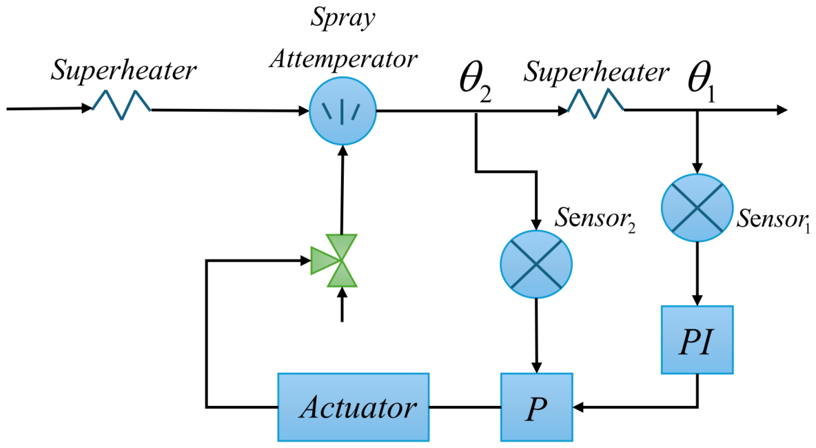
Figure 2 shows the cascade control system for main steam temperature. Steam is initially heated in the primary superheater before entering an attemperator, where the spray water flow is adjusted to control the temperature ${\theta }_2$. The steam then proceeds to the next superheater, with the final temperature ${\theta }_1$ being detected. The primary (PI) controller processes the deviation between ${\theta }_1$ and the setpoint, sending its output to the secondary (P) controller, which jointly regulates the attemperator spray water based on the ${\theta }_2$ deviation. This structure ensures rapid response and maintained temperature stability even under disturbances such as load variations.

In the state-space model, $x_1\left(k\right)$ and $x_2\left(k\right)$ denote the state vectors of the primary and secondary loops, respectively. The output of the secondary loop acts as the input to the primary loop, forming the cascade structure. Accordingly, the discrete-time state-space model can be written as:

$$\left\{\begin{array}{c}{x}_1(k+1)={\Phi }_1{x}_1\left(k\right)+{\Gamma }_1{y}_2\left(k\right)\hfill \\ x_2(k+1)={\Phi }_2{x}_2\left(k\right)+{\Gamma }_2{u}_2\left(k\right)+{\Psi }_{3}w\left(k\right)\hfill \\ y_1\left(k\right)=C_1{x}_1\left(k\right)\hfill \\ y_2\left(k\right)=C_2{x}_2\left(k\right)\hfill \end{array}\right.$$

where

$${\Gamma }_1=\left[\begin{array}{c}0.8367\\ 0.4273\\ 0.4437\end{array}\right],{\Gamma }_2=\left[\begin{array}{c}0.3425\\ 0.2542\\ 0.1008\end{array}\right],$$

$${\Phi }_1=\left[\begin{array}{ccc}0.6687& -0.0093& -0.0342\\ 0.8356& 0.9051& -0.0254\\ 0.3425& 0.2542& 0.1008\end{array}\right],{\Phi }_2=\left[\begin{array}{ccc}-0.0342& 0.2287& -0.0342\\ 0.3425& 0.8965& 0.0254\\ 0.2542& -0.0674& 0.9901\end{array}\right],$$

$${\Psi }_3=\left[\begin{array}{ccc}0.5& 0& 0\\ 0& 0.5& 0\\ 0& 0& 0.5\end{array}\right],C_1=\left[\begin{array}{ccc}0& 0& 0.111\end{array}\right],C_2=\left[\begin{array}{ccc}0& 0& 0.1\end{array}\right].$$

Among them, $y_1\left(k\right)$ represents the output of the inertial area, that is, the output of the main steam temperature, and $y_2\left(k\right)$ represents the output of the preheater area, that is, the output of the pre-heater steam temperature.

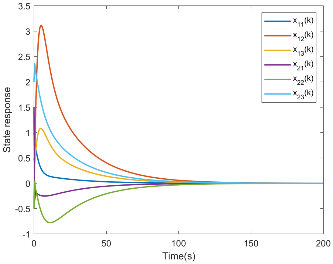
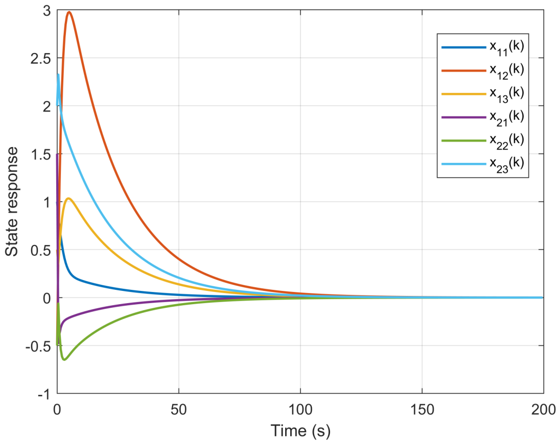
Example 1.

We assume that the gain matrices of the master controller and the auxiliary controller are, respectively:

$$\begin{array}{cc}\hfill K_p& =\left[\begin{array}{ccc}-0.2& -0.05& 0.01\end{array}\right],\hfill \\ \hfill K_i& ={10}^{-5}\times \left[\begin{array}{ccc}-0.2& -0.1& 0.2\end{array}\right],\hfill \\ \hfill K_2& =\left[\begin{array}{ccc}-0.05& -0.1& -0.05\end{array}\right].\hfill \end{array}$$

According to Theorem 1, using the Matlab/LMI Toolbox (R2024a), we can conclude that the system is stable and obtain the following matrices:

$$\widehat{P}=\left[\begin{array}{ccc}16.2061& -10.1239& 4.5578\\ -10.1239& 153.0906& 37.5390\\ 4.5578& 37.5390& 79.2495\end{array}\right], {\widehat{Q}}_1=\left[\begin{array}{ccc}1.7900& -3.3292& 0.6181\\ -3.3292& 10.8279& 1.3066\\ 0.6181& 1.3066& 17.6750\end{array}\right],$$

$${\widehat{Q}}_2=\left[\begin{array}{ccc}1.7900& -3.3292& 0.6181\\ -3.3292& 10.0523& 0.8739\\ 0.5854& 0.8739& 15.8528\end{array}\right], {\widehat{Q}}_3=\left[\begin{array}{ccc}1.6404& -3.1598& 0.5854\\ -3.1598& 10.8279& 1.3066\\ 0.6181& 1.3066& 17.7650\end{array}\right],$$

$$\widehat{T}=\left[\begin{array}{ccc}8.6906& -2.2391& -2.4865\\ -2.2391& 3.0537& -0.1448\\ -2.4865& -0.1448& 6.8018\end{array}\right].$$

If the initial condition is:

$$x_1\left(0\right)={\left[\begin{array}{ccc}1& -0.5& 0.5\end{array}\right]}^T, x_2\left(0\right)={\left[\begin{array}{ccc}1.5& -1.5& 2\end{array}\right]}^T$$

As shown in Figure 3, the system state responses indicate that under the action of the aforementioned gains of the master and auxiliary controllers, the system states tend toward zero. This implies that the Constant Temperature Control System is stable, and the system states can converge to zero.

The results of Example 1 confirm the feasibility of the LMI conditions in Theorem 1. Based on this theoretical verification, Example 2 further investigates the controller synthesis procedure of Theorem 2 and evaluates the resulting closed-loop performance.

Next, based on Theorem 2 proposed above, we will design the PI control law for the master controller and the P control law for the slave controller of system (9).

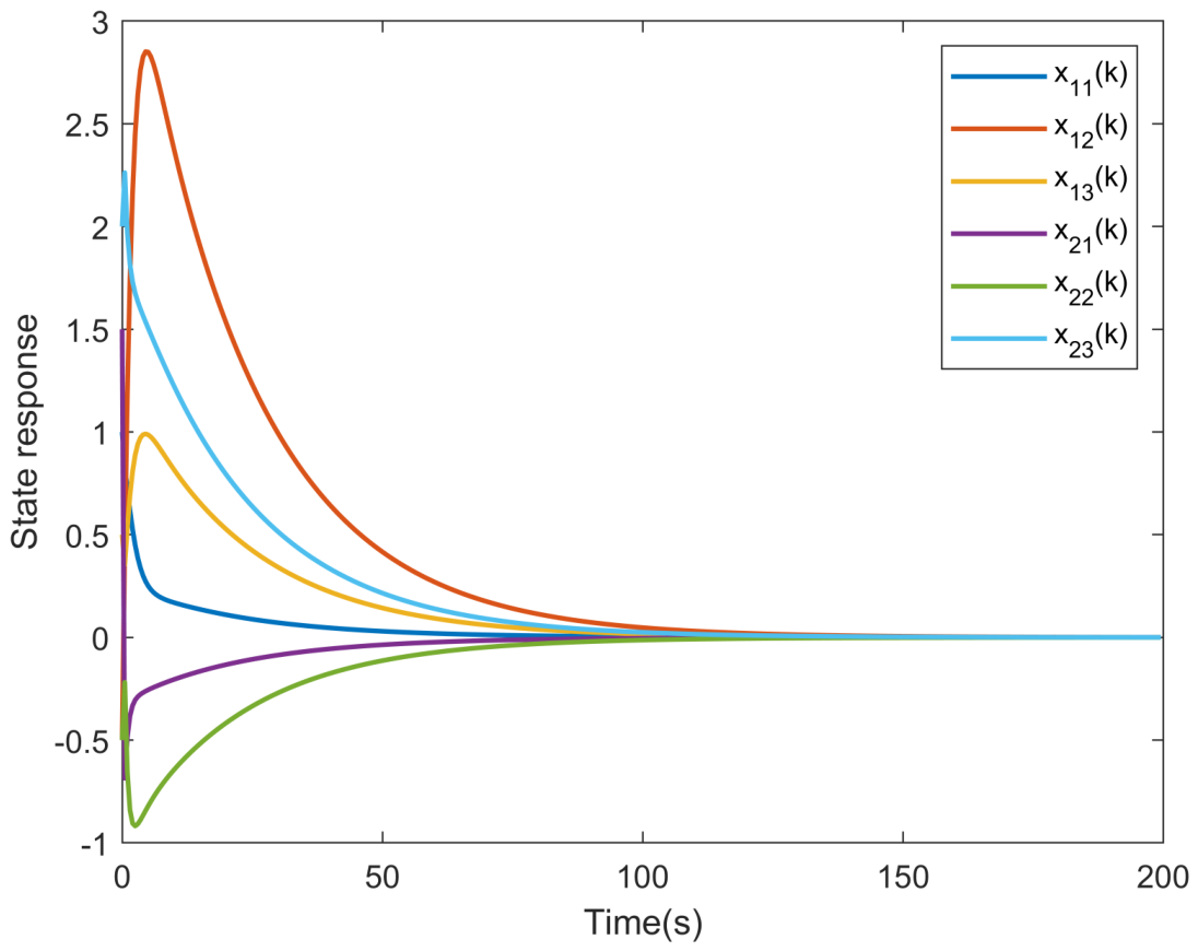
Example 2.

To design the state feedback control law for system (9), we follow Theorem 2. The parameter n is a configurable constant. For this implementation, we choose $n=2$ with sampling period $h=0.5$ s. The required matrices are computed via the MATLAB/LMI toolbox as follows:

$$\widehat{P}=\left[\begin{array}{ccc}6.0749& -5.9737& 1.1034\\ -5.9737& 46.6746& 10.0205\\ 1.1034& 10.0205& 29.0824\end{array}\right],{\widehat{Q}}_1=\left[\begin{array}{ccc}0.7422& -1.3194& 0.2363\\ -1.3194& 4.1270& 0.4422\\ 0.2363& 0.4422& 6.9285\end{array}\right],$$

$${\widehat{Q}}_2=\left[\begin{array}{ccc}0.7422& -1.3194& 0.2363\\ -1.3194& 4.1270& 0.4422\\ 0.2363& 0.4422& 6.9285\end{array}\right],{\widehat{Q}}_3=\left[\begin{array}{ccc}0.7422& -1.3194& 0.2363\\ -1.3194& 4.1270& 0.4422\\ 0.2363& 0.4422& 6.9285\end{array}\right],$$

$$\widehat{T}=\left[\begin{array}{ccc}5.4816& -0.5763& -1.0273\\ -0.5763& 7.3156& 3.0589\\ -1.0273& 3.0589& 4.7662\end{array}\right],W_p=\left[\begin{array}{c}-4.5547\\ -2.1466\\ -1.0151\end{array}\right],$$

$$W_i={10}^{-12}\times \left[\begin{array}{c}-0.0013\\ -0.0833\\ 0.1140\end{array}\right],W_2=\left[\begin{array}{c}-0.5928\\ -10.4001\\ -5.3058\end{array}\right],C_2=\left[\begin{array}{ccc}0& 0& 0.142\end{array}\right].$$

Based on Theorem 2, the parameters for both primary and secondary controllers are determined as follows:

$$\begin{array}{cc}\hfill & K_p={\left({\widehat{P}}^{-1}{W}_p\right)}^T=\left[\begin{array}{ccc}-0.9375& -0.1794& 0.0625\end{array}\right],\hfill \\ \hfill & K_i={\left({\widehat{P}}^{-1}{W}_i\right)}^T={10}^{-14}\times \left[\begin{array}{ccc}-0.4643& -0.3518& 0.5307\end{array}\right],\hfill \\ \hfill & K_2={\left({\widehat{P}}^{-1}{W}_2\right)}^T=\left[\begin{array}{ccc}-0.3096& -1.3021& -0.3443\end{array}\right].\hfill \end{array}$$

If the initial conditions are:

$$x_1\left(0\right)={\left[\begin{array}{ccc}1& -0.5& 0.5\end{array}\right]}^T, x_2\left(0\right)={\left[\begin{array}{ccc}1.5& -1.5& 2\end{array}\right]}^T$$

As demonstrated by the system response curves in Figure 4, the system states approach zero at approximately 150 s, which directly substantiates their convergence properties. Consequently, the closed-loop control system is confirmed to be stable, and the controller gain obtained via LMI guarantees that the system states converge effectively to zero.

To the best of our knowledge, limited theoretical results are available for systems operating under nonlinear discrete cascade PI-P controllers. To demonstrate the effectiveness of the proposed approach, a comparative simulation study was carried out under identical conditions, utilizing a controller derived from Corollary 1 of this paper by removing the integral term.

Based on Corollary 1, the parameters for both primary and secondary controllers are determined as follows:

$$\begin{array}{cc}\hfill & K_p={\left({\widehat{P}}^{-1}{W}_p\right)}^T=\left[\begin{array}{ccc}-0.8582& -0.1639& 0.0466\end{array}\right],\hfill \\ \hfill & K_2={\left({\widehat{P}}^{-1}{W}_2\right)}^T=\left[\begin{array}{ccc}-0.2252& -1.2797& -0.1254\end{array}\right].\hfill \end{array}$$

As illustrated by the state response curves in Figure 5, the system states converge to zero at approximately 150 s as well.

Due to the fact that the dynamic behavior of augmented-state systems is determined by multiple state variables, the response of a single output channel is insufficient to comprehensively measure the overall operational performance of the system. Therefore, this paper adopts the state vector norm ${\parallel x\left(k\right)\parallel }_2=\sqrt{x_1^T\left(k\right)x_1\left(k\right)+x_2^T\left(k\right)x_2\left(k\right)}$ as a comprehensive evaluation indicator to aggregate the overall variation trend of all state components, enabling a more accurate characterization of the system’s dynamic characteristics. Based on this indicator, the time required for the state norm to decay to 1% of its initial value is defined as the settling time of the system, which quantifies the convergence speed.

The work presented in [39] employs an LQR-based approach for PID controller tuning. Since [39] and the proposed method are developed under different modeling assumptions and design objectives, the former is cited here to illustrate an alternative controller design strategy rather than as a benchmark for performance comparison.

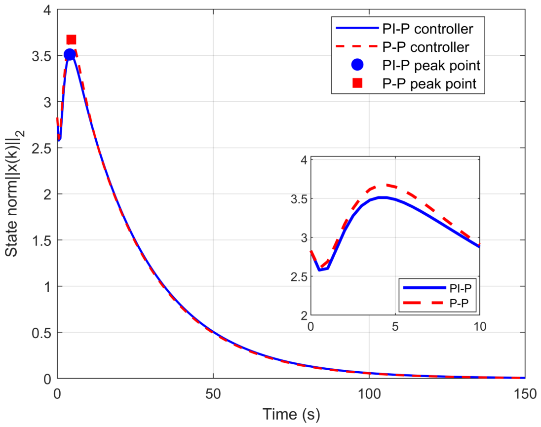
Based on the time-varying state norm curves under the two controllers shown in Figure 6, the integral absolute error (IAE) and integral square error (ISE) are calculated, and the results are presented in

Table 2. Comparison of Controller Performance Metrics.

Metric	PI-P Controller	P-P Controller
Peak time (s)	4.00	4.50
Norm peak	3.5106	3.6713
Overshoot (%)	24.12	29.8
ISE	198.0861	203.5358
IAE	98.3048	98.4031

.

The state norm is used here as an auxiliary indicator to characterize the overall convergence behavior of the augmented state-space model, while the control performance is further evaluated using conventional metrics such as peak overshoot, ISE, and IAE shown in Table 2. Comparing the time-varying state norm trajectories in Figure 6 with the control performance metrics in Table 2 reveals that the PI-P controller outperforms the P-P controller in terms of overall control performance. The PI-P controller yields a lower peak state norm and a much smaller overshoot, effectively reducing initial shocks and fluctuations. Meanwhile, its ISE and IAE values are significantly lower than those of the P-P controller, demonstrating superior error suppression, faster convergence, and higher control accuracy. These results confirm the dual advantages of the PI-P controller in both dynamic response and steady-state performance.

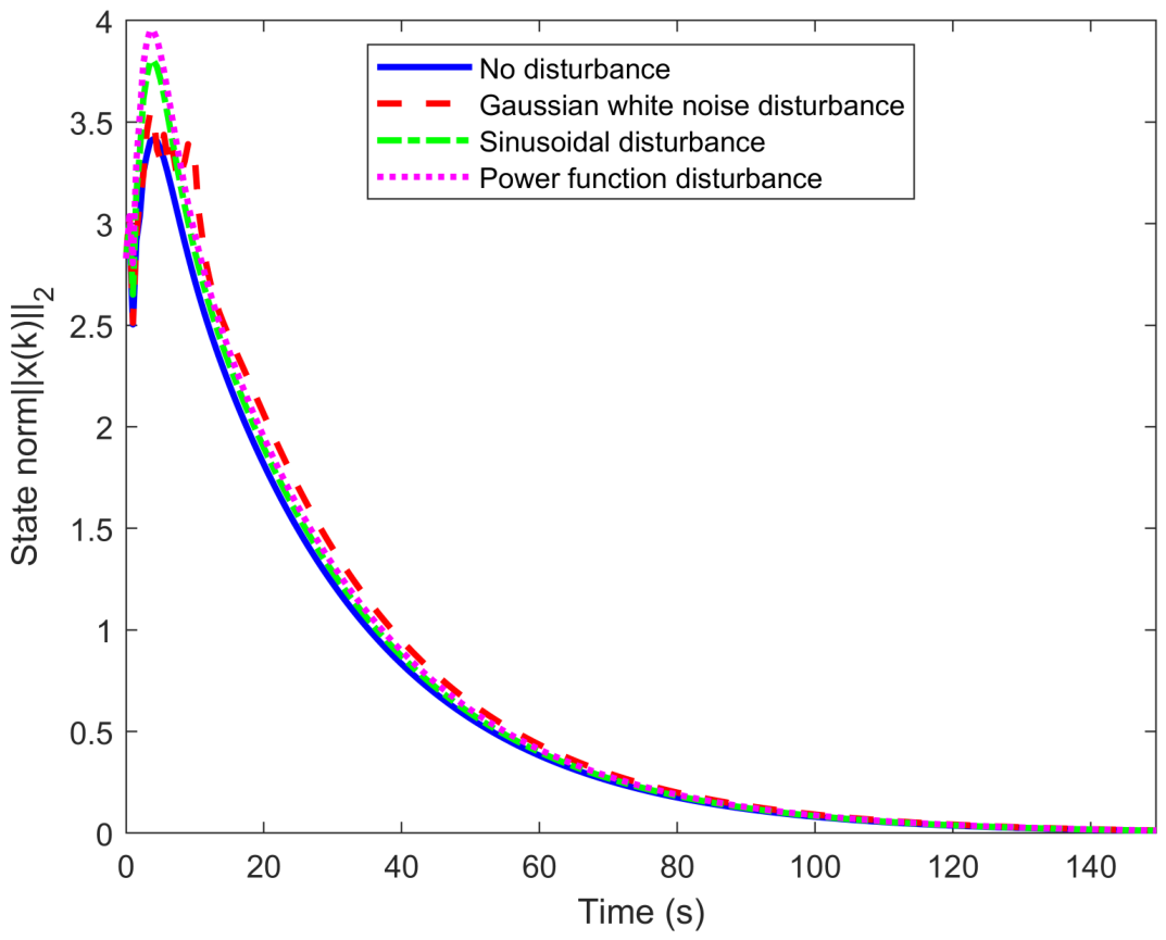
To evaluate the disturbance rejection capability of the designed controller under practical operating conditions, three representative external disturbances, namely Gaussian white noise, sinusoidal disturbance, and power-function disturbance, are injected into the control input channel $u_2\left(k\right)$. These disturbances are applied only during the interval $k\le 100$. By comparing the state norm response trajectories under both disturbance-free and disturbed conditions, as well as the post-disturbance recovery behavior for $k>100$, the controller’s ability to suppress external disturbances and restore the system to its equilibrium state can be comprehensively evaluated.

(1)

Gaussian white noise disturbance: $d_1\left(k\right)\sim \mathcal{N}(0,{\sigma }^2)$, $\sigma =0.2$, $k\le 100$.

(2)

Sinusoidal disturbance: $d_2\left(k\right)=1.2e^{-0.8k}sin\left(0.1k\right)$.

(3)

Power function disturbance: $d_3\left(k\right)=0.15k^{-1.8}$.

The state vector norm trajectories of the proposed system under the aforementioned three types of disturbances are shown in Figure 7.

The simulation results demonstrate that under the influence of three typical disturbances, the system state norm converges rapidly and remains stable. This fully indicates that the controller designed in this paper possesses strong anti-interference capability, can effectively handle different types of external disturbances, and ensures stable system operation in complex environments.

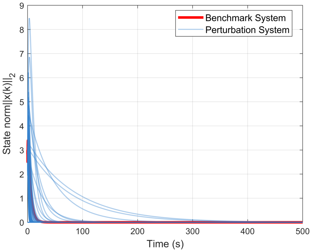
Unlike Figure 7, which evaluates disturbance rejection against external inputs, Figure 8 focuses on robustness with respect to model uncertainty. To evaluate this robustness, a Monte Carlo simulation comprising 200 independent trials was conducted. In each trial, random perturbations of $\pm 15\%$ were independently applied to the discrete-time state-space matrices ${\Phi }_1$ and ${\Phi }_2$, the input matrices ${\Gamma }_1$ and ${\Gamma }_2$, and the nonlinear distribution matrix ${\Psi }_3$ to represent model uncertainty. The resulting state-norm trajectories, shown in Figure 8, demonstrate that the proposed controller maintains stability and acceptable performance despite significant parameter variations.

Remark 12.

In engineering scenarios such as thermoelectric temperature control, nonlinear factors like saturation and dead zone significantly increase the complexity of system dynamics. Wide-range operating variations induce strongly nonlinear heat exchange, thereby breaking the linear dependence between the temperature change rate and the control input [23,24]. The stability of nonlinear systems is highly sensitive to initial conditions, which can easily lead to response divergence. Therefore, in PI controller design, it is necessary to adopt a customized state-space model and incorporate Lyapunov functions for stability analysis to ensure the effectiveness of the control method.

Remark 13.

Research on PI controllers for nonlinear discrete cascade systems carries dual significance in theoretical and practical domains. Theoretically, it addresses the under-explored integration of nonlinear discrete dynamics with cascade PI control, establishing systematic design and stability analysis methods to advance control theory for complex systems. Practically, it resolves key industrial challenges by developing coordinated parameter tuning mechanisms that mitigate common issues like response lag and overshoot, thereby enhancing control precision and reducing commissioning costs while modernizing traditional control methodologies.

5. Conclusions

To address the control challenges of nonlinear discrete cascade systems, this paper constructs an extended state-space model incorporating integral terms, achieving collaborative state feedback modeling and tuning of PI-P controllers. By effectively handling nonlinear elements via the sector-bounding method and utilizing Lyapunov functionals with LMI tools, the proposed method ensures asymptotic stability of the system. It simultaneously eliminates steady-state error through the primary loop PI control while preserving the rapid disturbance rejection advantage of the secondary loop P control, meeting the dual requirements for offset-free performance and fast response. Simulation results on a main steam temperature control system demonstrate the effectiveness of the proposed method in nonlinear discrete cascade systems, showing improved dynamic response and disturbance rejection compared to conventional sequential tuning approaches. The theoretical contribution lies in establishing a systematic design and stability analysis framework for nonlinear discrete cascade control. The proposed method has potential application value and offers theoretical support for control upgrades in relevant industrial fields. Future work will extend this approach to consider practical engineering constraints, and also explore integration with state observers and adaptive algorithms to address more complex industrial scenarios.