Article

A Memristive-System-Based Hysteresis Model for a Compact Pneumatic Artificial Muscle

Department of Mechatronics and Automation, Faculty of Engineering, University of Szeged, 6725 Szeged, Hungary
*
Authors to whom correspondence should be addressed.
Actuators 2026, 15(5), 257; https://doi.org/10.3390/act15050257
Submission received: 29 March 2026 / Revised: 23 April 2026 / Accepted: 29 April 2026 / Published: 2 May 2026

Abstract

Pneumatic artificial muscles exhibit pronounced hysteresis in the force-contraction domain, which complicates accurate force modeling under pressure-dependent operation. This work presents a discrete-time quasi-static hysteresis model for a compact pneumatic artificial muscle using a memristive system-based branch-memory formulation. The model combines separate loading and unloading force surfaces through a bounded internal state and is evaluated on experimental data acquired at a force-change rate of 4 N / s . Measurements were performed at 13 pressure levels from 0 to 0.6 MPa in 0.05 MPa increments, with 32 unloading points and 32 loading points per pressure level and five repetitions for each operating condition. Representative branch curves were obtained by median reduction in the repeated measurements, and the loading and unloading surfaces were identified with the five-parameter Sárosi–Fabulya exponential-bilinear function. The state update parameter was evaluated over a fixed grid, and the best loop reconstruction on the present dataset was obtained for the hard-switching case α = 1 . Benchmark comparisons with Prandtl–Ishlinskii, discrete Preisach, Maxwell-slip, and sampled Bouc–Wen-type models show that Preisach and Bouc–Wen provide higher loop-reconstruction accuracy. The proposed memristive formulation should not be interpreted as a best-fit benchmark model, but as a low-order global branch-memory representation that preserves pressure dependence and branch asymmetry within a single analytical framework over the investigated quasi-static operating range.

1. Introduction

Pneumatic artificial muscles (PAMs) are widely used for robotics, mechatronics, and bioinspired actuators because they combine a high force-to-weight ratio, compactness, compliance, and mechanical simplicity. However, these same advantages are accompanied by pronounced nonlinearities. For a given actuator, the generated force depends not only on pressure and contraction, but also on the path by which the operating point is reached. This path dependence is observed as hysteresis between loading and unloading branches, and it remains one of the main reasons why accurate force estimation and model-based control are difficult in PAM-driven systems [1,2,3,4,5,6,7,8]. Control-oriented PAM studies have therefore explored piecewise-affine modeling, switching model predictive control, adaptive compensation under dead zones, hybrid PI-NARMAX identification, and double-air-chamber actuator variants in order to improve prediction and tracking under hysteresis and nonlinearity [9,10,11,12,13].
The PAM literature already contains several strong hysteresis-modeling families. Preisach formulations represent hysteresis by a weighted superposition of relay operators, Prandtl–Ishlinskii models use superposed play operators, Bouc–Wen models introduce a low-order hysteretic state, and Maxwell-slip models describe hysteresis through parallel elasto-slip elements [14,15,16]. More recent work has also reported comprehensive dynamic models under varying frequency and load, improved generalized Bouc–Wen models, fractional-order Bouc–Wen formulations, and mechanically grounded constitutive descriptions based on chain extensibility [4,17,18,19]. These approaches are effective, but they are not equally convenient when the modeling objective is narrow and pragmatic, namely to preserve experimentally identified loading and unloading surfaces with the smallest possible additional memory structure.
The present study adopts that narrower objective. Instead of treating force rate as a free scheduling variable, only the quasi-static dataset acquired at a force-change rate of 4 N / s is used. The actuator platform and quasi-static hysteresis dataset are consistent with the previous comparative CPAM study of Csikós et al. [20]; the present manuscript uses that same measurement framework for memristive-system-based branch modeling. At this operating condition, separate loading and unloading surfaces are identified for both excitation force-contraction (EFC) and measured force-contraction (MFC) data using the five-parameter Sárosi–Fabulya function [21,22]. Those branch surfaces are then combined in MATLAB R2024a through a bounded internal state variable.
In this restricted setting, the internal state is not introduced as a first-principles constitutive variable. It is introduced as the minimal branch-memory variable required once the measured data show that two different quasi-static force values can occur at the same ( ε , p ) pair depending on the previously traversed path. The state therefore has a deliberately narrow interpretation: it is a coarse-grained reduced coordinate that aggregates unresolved internal effects into branch occupancy, rather than a unique physical descriptor of braid friction, bladder viscoelasticity, or end-effect deformation.
This formulation is useful because it fits naturally into generalized memristive-system theory. Chua introduced the memristor as a memory-bearing constitutive relation between electrical variables [23], and Chua and Kang generalized that concept to state-dependent systems in which the output depends on both the present input and one or more internal states [24]. Broader discussions of memory effects in complex materials, memristive/memcapacitive/meminductive systems, and comparative device-model behavior likewise support the use of generalized state-dependent language when the objective is phenomenological representation rather than strict material classification [25,26,27]. Later work has clarified that mechanically or fluidically hysteretic systems may be modeled in this broader memristive-system sense without claiming that they are ideal material memristors in the strict electrical sense [28,29,30,31,32]. Recent nanofluidic and angstrom-fluidic studies further reinforce that point by demonstrating memristive ionic transport, long-term memory, logic behavior, and pore-deformation-driven state dependence in non-solid-state platforms [33,34,35,36,37,38,39,40]. That distinction is central here. The claim of this paper is a modeling claim, not a material-identity claim.
In this paper, that memristive-system interpretation is realized through a bounded branch-weighting state formulation that can represent either hard switching or smoother blending between the identified loading and unloading surfaces. The explicit state-dependent mixture is introduced in Section 2.3.
The contribution of the paper is therefore specific and limited. First, it identifies separate loading and unloading branch surfaces at 4 N / s using the five-parameter Sárosi–Fabulya force-contraction representation. Second, it embeds those branch surfaces in a low-order memristive-system-based hysteresis model with a bounded internal state. Third, it retains both EFC and MFC surface families in the MATLAB workflow so that the branchwise hysteresis reconstruction can be evaluated from two closely related force-contraction representations.
The remainder of the manuscript is organized as follows. Section 2 summarizes the relevant hysteresis-model families and the mechanical-electrical analogy used in the paper. Section 3 describes the actuator variables, the fixed-rate measurement protocol, and the branch-surface identification procedure. Section 4 introduces the memristive-state coupling law and the evaluation setup. Section 5 discusses the resulting branchwise hysteresis representation and its present scope. Section 6 concludes the paper.

2. Background

2.1. Established Hysteresis Model Families

Several model families are established in the PAM hysteresis literature, and the proposed low-order branch-memory model is easier to position when their canonical structures are stated explicitly. A classical Preisach representation writes the output as a weighted superposition of relay operators [41],
y ( t ) = α β μ ( α , β ) γ α β [ u ] ( t ) d α d β ,
where u ( t ) is the input, y ( t ) is the output, γ α β [ u ] ( t ) is an elementary relay with thresholds α and β , and μ ( α , β ) is the Preisach density. The Preisach framework is highly expressive because it can represent complex branch memory through a distributed set of switching elements. Its main limitation for the present problem is that this flexibility comes with a higher identification burden, since the density over the Preisach plane must be estimated and regularized. For the present quasi-static PAM problem, it is therefore a useful benchmark family, but less attractive when a low-state representation is desired.
A Prandtl–Ishlinskii (PI) model is commonly written as
y ( t ) = p 0 u ( t ) + i = 1 N q i P r i [ u ] ( t ) ,
where p 0 is the direct gain, q i are operator weights, r i are play thresholds, and P r i denotes the play operator with threshold r i [14,15]. PI-type models are attractive because their structure is often easier to identify and invert than Preisach-type formulations, which is why they are widely used in hysteresis compensation and control-oriented modeling. However, standard PI forms may require modification when the measured loop is strongly asymmetric or when branch transitions are not captured well by a simple superposition of play operators. For this reason, PI-type models are relevant references, but they are not always the most economical description of the branch-dependent quasi-static behavior considered here.
Recent PAM studies also use generalized and fractional-order Bouc–Wen variants when branch asymmetry or frequency dependence cannot be captured satisfactorily by simpler operator models [17,18]. A Bouc–Wen-type formulation introduces a low-order hysteretic state,
z ˙ = A u ˙ β | u ˙ | | z | n 1 z γ u ˙ | z | n , y ( t ) = k u u ( t ) + k z z ( t ) ,
where z ( t ) is the hysteretic internal state, A, β , γ , and n are shape parameters, and k u and k z are output gains. This Bouc–Wen coefficient β is unrelated to the Preisach threshold β . Bouc–Wen-type models are structurally closer to low-order state-space descriptions because hysteresis is represented through a small number of internal states rather than through many elementary operators. Their main advantage is descriptive economy, but parameter interpretation and identification can become difficult because the coefficients are strongly coupled, and additional terms are often needed when asymmetry or rate effects are pronounced.
Maxwell-slip models represent hysteresis through the parallel combination of elementary elasto-slip components,
y ( t ) = i = 1 N y i ( t ) , y i ( t ) = k i u ( t ) x i ( t ) ,
where N is the number of parallel elements, y i is the output of the i-th element, k i is its stiffness, and x i ( t ) is the corresponding internal slip or displacement state. Maxwell-slip models provide an intuitive interpretation in terms of distributed sticking and slipping behavior and can reproduce quasi-static hysteresis effectively. Their accuracy, however, typically depends on the number of elementary elements used, which again introduces a complexity-order trade-off. Relative to such multi-element models, the present work seeks a lower-order branch-memory representation.
Taken together, these model families illustrate the central trade-off in hysteresis modeling: Preisach, PI, and Maxwell-slip models achieve flexibility through multiple internal elements, whereas Bouc–Wen achieves it through a smaller differential-state model. The present manuscript follows the low-order state direction, but instead of postulating a generic operator family from the outset, it starts from experimentally visible loading and unloading surfaces and introduces a single bounded internal state to encode branch memory.

2.2. Mechanical-Electrical Analogy Choice

Memristive modeling of a pneumatic artificial muscle requires an explicit bridge between mechanical and electrical variables. That bridge is not unique in the literature. The apparent disagreement over whether an electrical inductor corresponds to a mechanical spring or to a mechanical mass reflects the use of different, but standard, analogy choices rather than a contradiction.
Two analogy families are established in the mechanical-electrical literature. In the impedance analogy, force is mapped to voltage and velocity is mapped to current, so inertial behavior is associated with inductive storage, viscous damping with resistance, and spring compliance with capacitance [42,43]. In the mobility (admittance) analogy, force is mapped to current and velocity is mapped to voltage, so inertial behavior is associated with capacitance and elastic storage is associated with inductive behavior [42,44,45]. A second source of notation drift is that some authors describe the spring through stiffness, while others use compliance. This changes the parameter attached to the analogous circuit element without changing the underlying analogy itself. Engineering mechanics and bond-graph mem-model studies make this bridge explicit by writing displacement-dependent damping and integral-displacement elasticity in direct constitutive analogy with memristive and memcapacitive elements, including mechanical “mem-dashpot” and “mem-spring” interpretations [46,47,48].
For the present manuscript, the impedance analogy is used. This choice keeps force as the effort-like variable and velocity as the flow-like variable, which aligns directly with the force-oriented hysteresis surfaces identified in the experiments [42,43]. Table 1 summarizes the equation-level correspondences and keeps the mobility column only as a comparative reference, making the source of the inductor-mass versus inductor-spring distinction explicit.
The paper therefore does not argue that compact PAMs require a unique mechanical-electrical analogy. It fixes the impedance analogy so that hysteretic, elastic, and dissipative terms can be written in a consistent state-equation form.

2.3. Generalized Memristive-System Interpretation

With that analogy in place, the relevant memristive-system idea is the generalized state-dependent form introduced by Chua and Kang [24]. In its canonical current-controlled form,
U ( t ) = 1 M ( x , I , t ) I ( t ) , x ˙ = f ( x , I , t ) ,
where U and I are port variables, x is an internal state, and M ( · ) is the memristive function. For the present work, the important feature is structural: the observable output depends on both the current excitation and an internal state carrying part of the system history. In this paper, that role is assigned to the bounded branch variable x through the state-dependent branch mixture
F ^ ( ε , p , x ) = x F load ( ε , p ) + ( 1 x ) F unload ( ε , p ) ,
where F ^ is the estimated force, ε is contraction, p is pressure, and x [ 0 , 1 ] is the internal state weighting the loading and unloading surfaces. In the present MATLAB implementation, the state is updated in discrete time and acts primarily as a branch-memory variable.
The use of x can be justified more systematically without claiming a microscopic constitutive derivation. At the fixed quasi-static rate used here, the experiments show two limiting force surfaces for the same ( ε , p ) pair, one reached during monotone contraction and one during monotone expansion. A single-valued static surface F ( ε , p ) is therefore insufficient. If the unresolved internal configuration of the actuator is denoted abstractly by a higher-dimensional variable z, then the present model may be interpreted as a reduced-order projection that keeps only the dominant observable consequence of z, namely branch occupancy. In that reduced view, x 0 corresponds to the unloading manifold, x 1 corresponds to the loading manifold, and intermediate values represent a possible finite transition layer. The proposed state is therefore a coarse-grained phenomenological reduction in branch memory rather than a claim that one uniquely identified physical variable has been derived from first principles.
This interpretation should not be overstated. The manuscript does not claim that the compact pneumatic artificial muscle is an ideal electrical memristor in the strict sense debated in the memristor literature [28,29]. It claims only that the observed hysteretic force response can be represented in generalized memristive-system form. Reviews of memory effects and generalized memelements likewise emphasize that state-bearing behavior occurs across broader classes of systems than idealized electronic material memristors alone [25,26]. Recent mechanically gated ionic and nanofluidic memristive devices reinforce that broader cross-domain interpretation by showing that memory-bearing input-output behavior is not restricted to solid-state electronic media [30,31,32,33,34,35,36,37,38,39,40].

3. Materials and Methods

3.1. Actuator and Variables

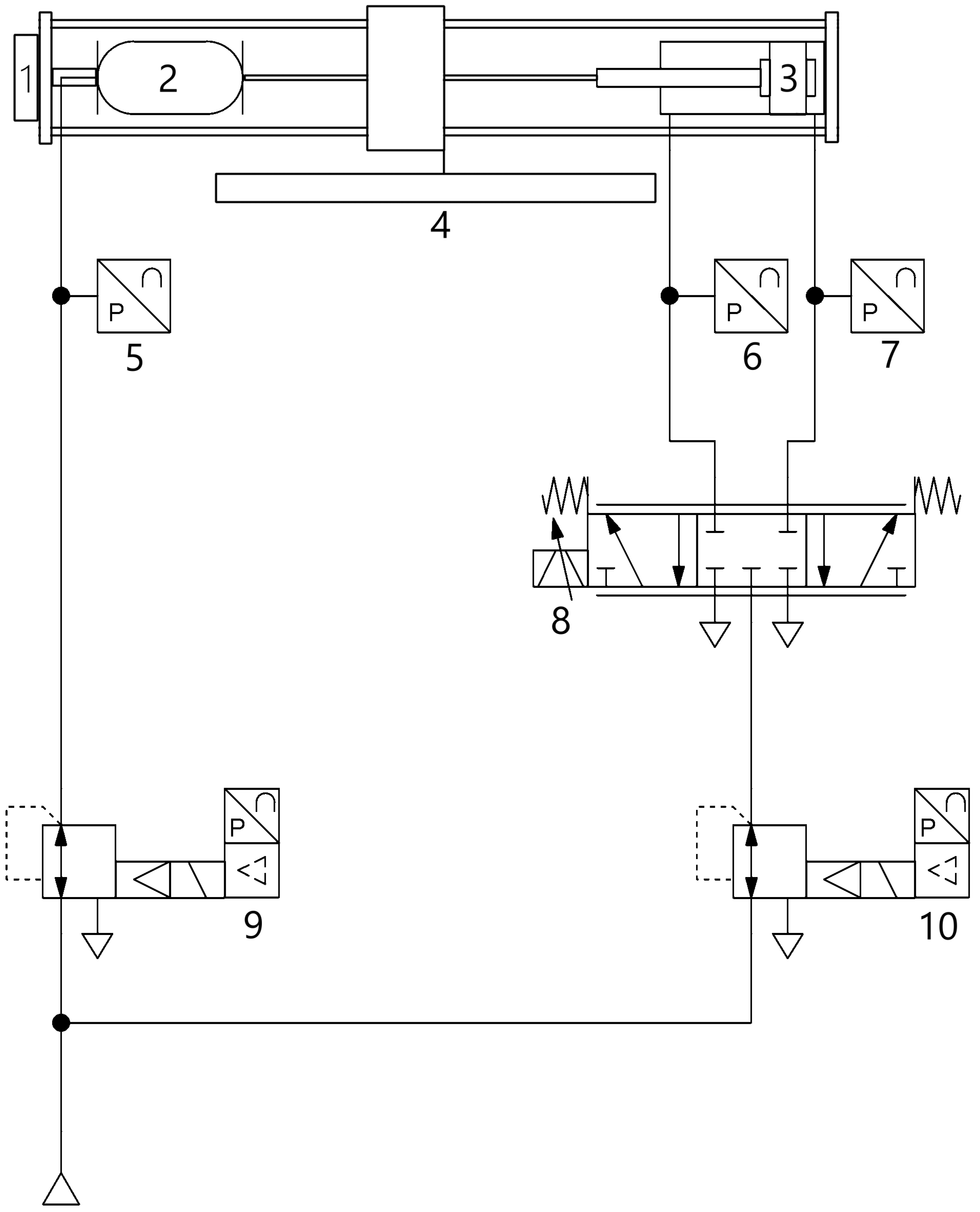
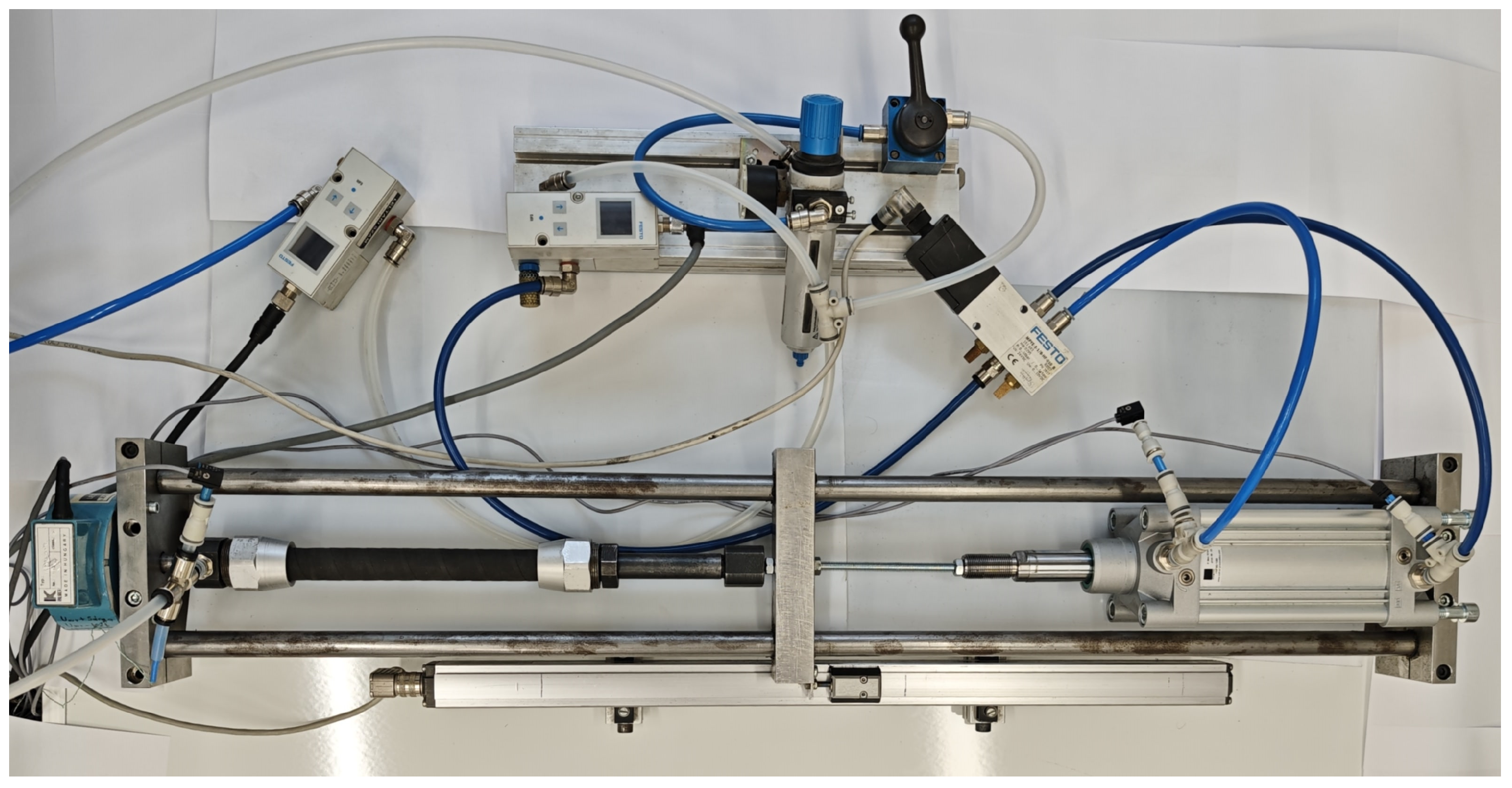
The actuator under study is a compact pneumatic artificial muscle based on a McKibben-type outer structure with an internal spring-rod arrangement. The compact spring-rod architecture and the full force-controlled measurement rig were described in detail previously by Csikós et al. [20]. Therefore, only the features directly relevant to the present quasi-static hysteresis identification are summarized here. The model variables are the internal pressure p, the contraction ε , and the measured actuator force F. Throughout the paper, contraction is used as the independent kinematic coordinate along each measured branch, and pressure is treated as the external operating parameter. Figure 1 and Figure 2 show the experimental setup and its schematic representation.
The notation deliberately uses ε for contraction rather than k in order to avoid conflict with the standard stiffness symbol. In the identified equations below, ε is used exactly in the scaling adopted by the MATLAB fitting workflow.
The cart, piston rod, tested muscle, and load cell were aligned along a single axis on linear guide rails in order to minimize side loads and bending moments on both the muscle and the load cell. The numbered elements in Figure 2 are as follows:
(1)
Uniaxial load cell, type KALIBER 8923-200 kg (Budapest, Hungary); the load-cell signal was processed with a ClipX BM40 unit (Göttingen, Germany).
(2)
Tested muscle (CPAM).
(3)
Double-acting pneumatic cylinder, type HAFNER HIF80/100 (Halászi, Hungary), used to apply the controlled excitation force.
(4)
Linear position sensor, type BALLUF BTL5-S101-M0500-P-S32 (Veszprém, Hungary), used to determine the cart position and thereby the muscle contraction.
(5)
Pressure sensor, type FESTO SPTE-571484 B9 (Budapest, Hungary), mounted on one cylinder port.
(6)
Pressure sensor, type FESTO SPTE-571484 B9 (Budapest, Hungary), mounted on the other cylinder port.
(7)
Pressure sensor, type FESTO SPTE-571484 B9 (Budapest, Hungary), mounted on the tested muscle.
(8)
Proportional valve, type FESTO MPYE-5-1/8-HF-010 B (Budapest, Hungary).
(9)
Pressure regulator for the tested muscle, type FESTO VPPM-6L-L-1-G18-0L6H-V1N-S1C1 (Budapest, Hungary).
(10)
Electro-pneumatic pressure regulator for the cylinder supply, type FESTO VPPM-6L-L1-G18-0l6H-V1N-S1C1 (Budapest, Hungary).
By commanding the regulator output and the proportional valve, a prescribed net force was generated at the piston-rod interface. The pressure of the tested muscle was controlled independently, while the far end of the load cell was fixed to the stationary frame of the rig.
The excitation force produced by the pneumatic cylinder was calculated from the measured chamber pressures and piston areas, following the previous comparative CPAM study [20]. Let P pos and P neg denote the absolute pressures in the cap-end and rod-end chambers, respectively, and let A pos and A neg be the corresponding effective piston areas, with A neg = A piston A rod on the rod side. The net axial force exerted by the cylinder on the cart was then computed as
F excitation ( t ) = P pos ( t ) A pos P neg ( t ) A neg

3.2. Measurement Protocol

The dataset was recorded at a force-change rate of 4 N / s . The measurement protocol follows the previous comparative CPAM study [20]. Before the hysteresis measurements, the actuator was characterized under the maximum operating conditions used in that study. At the maximum loading condition, the compact PAM reached a stretched state of approximately 1.5 % relative to its free length at atmospheric pressure. This limited extension, compared with the larger extension of the commercial reference muscle reported in [20], was attributed to the internal spring-rod arrangement of the compact actuator, which produces a stiffer tensile response during extension. In the present manuscript, that stretched configuration is used as the repeatable pre-tensioned start state for each quasi-static hysteresis cycle.
The pressure range spans
p { 0 , 0.05 , 0.10 , , 0.60 } MPa ,
which gives 13 pressure levels in total. This pressure grid was selected for two reasons. First, it spans the rated operating range of the investigated CPAM under the quasi-static conditions considered here. Second, the same 0–0.6 MPa range with 0.05 MPa increments was used in our previous experimental characterization of the same actuator [20], which keeps the present results directly comparable with that earlier dataset.
At the beginning of each measurement sequence, the CPAM was brought close to its maximum stretched state and held there for 10 s . This dwell acted as a conditioning step to stabilize the braid and bladder configuration and to reduce short-term history effects before the excitation-force ramp started.
For each pressure level, the following sequence was applied:
1.
The muscle pressure was set to the prescribed level.
2.
The excitation force was adjusted so that the muscle returned to the pre-tensioned stretched state and was then held for 10 s .
3.
The unloading branch, which corresponds to contraction in the notation of this paper, was recorded by ramping the excitation force approximately linearly at 4 N / s from the stretched state toward the maximum contraction reachable at that pressure; the retained branch contains 32 sampled setpoints.
4.
The loading branch, which corresponds to expansion, was then recorded by reversing the ramp to approximately + 4 N / s until the pre-tensioned state was reached again; this retained branch also contains 32 sampled setpoints.
5.
Steps 1–4 were repeated five times.
As discussed in the previous paper [20], the first point immediately after the pre-tensioning dwell may deviate from the prescribed quasi-static ramp condition. The present manuscript therefore works with the retained quasi-static branch samples used for the MATLAB identification. For each retained branch position, the five repeated force measurements were reduced to a representative value by taking the median force. This yields one representative unloading curve and one representative loading curve for each pressure level.
The retained identification dataset is larger than the phrase “32 sampled setpoints” may suggest. The 32 points refer to one branch at one pressure level. Across the 13 pressure levels used here, this corresponds to 13 × 32 = 416 representative samples per branch after median reduction and 13 × 32 × 5 = 2080 raw samples per branch before reduction. Since each branch surface contains five fitted coefficients, the representative dataset provides approximately 416 / 5 = 83.2 samples per fitted parameter. The median was used to obtain a robust branch representative at each retained setpoint rather than to shrink the operating domain; however, it necessarily suppresses repeat-to-repeat dispersion near reversal, so uncertainty should be assessed separately from the point estimates reported below.

3.3. Branch-Wise Force Representation

The measured force-contraction relation was represented separately for unloading and loading using the five-parameter Sárosi–Fabulya function [21,22]
F ( ε , p ) = p + a 1 e a 2 ε + a 3 ε p + a 4 p + a 5
This structure combines an exponential dependence on contraction with a bilinear correction term in ε p and a linear pressure term. In the present manuscript, this branch function is used as a low-parameter analytical approximation rather than as a claim of universal optimality against all possible regressors. The main reason for this choice is pragmatic: the proposed hysteresis model requires smooth branch surfaces that are easy to identify, easy to evaluate numerically, and simple to embed in the internal-state blending law. Given the limited size of the available quasi-static dataset, a five-parameter analytical surface was considered more appropriate than a higher-capacity regression or machine-learning model.
It was fitted separately for the loading and unloading branches and retained for two surface families used in the MATLAB workflow:
  • Excitation force-contraction (EFC).
  • Measured force-contraction (MFC).
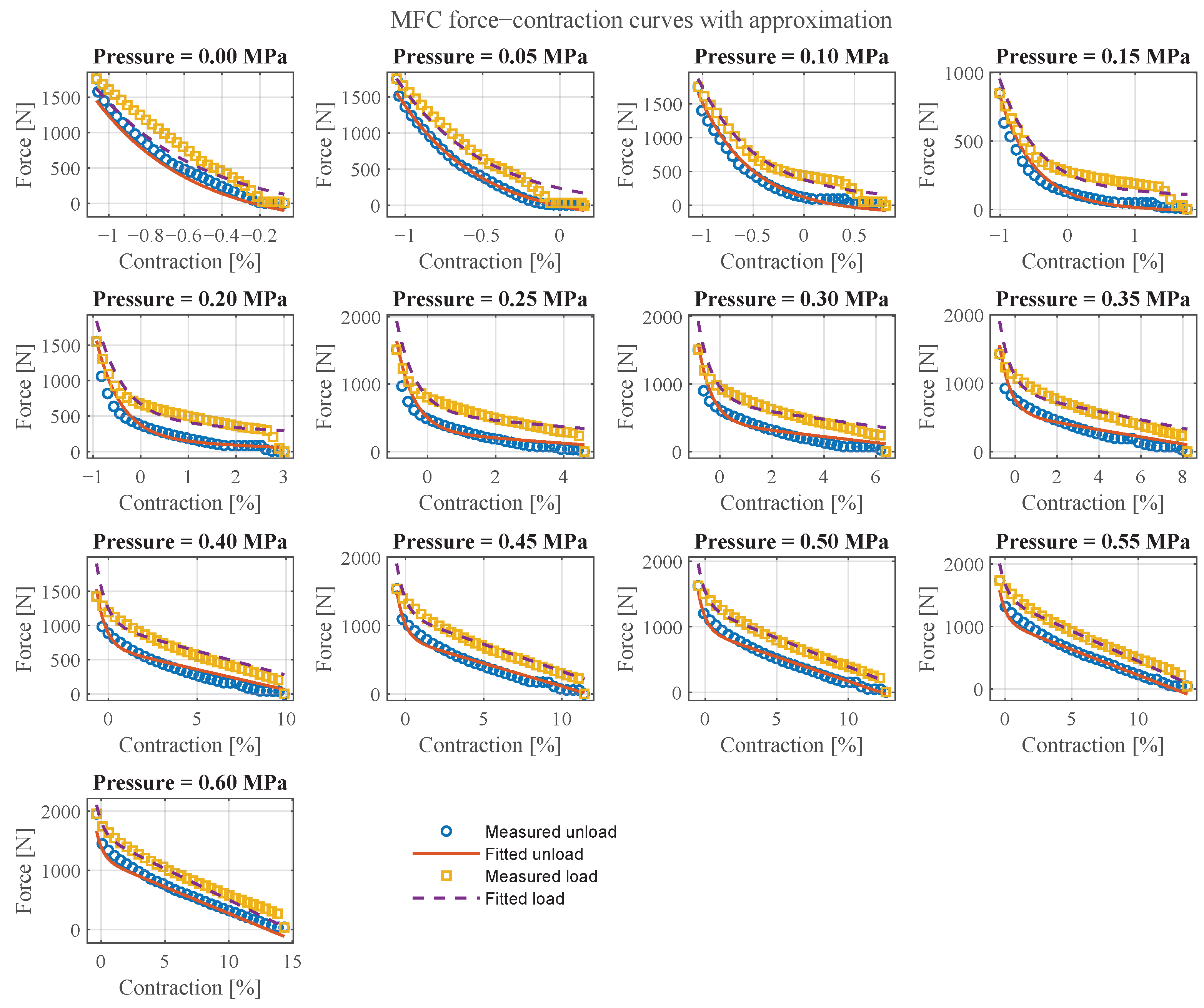
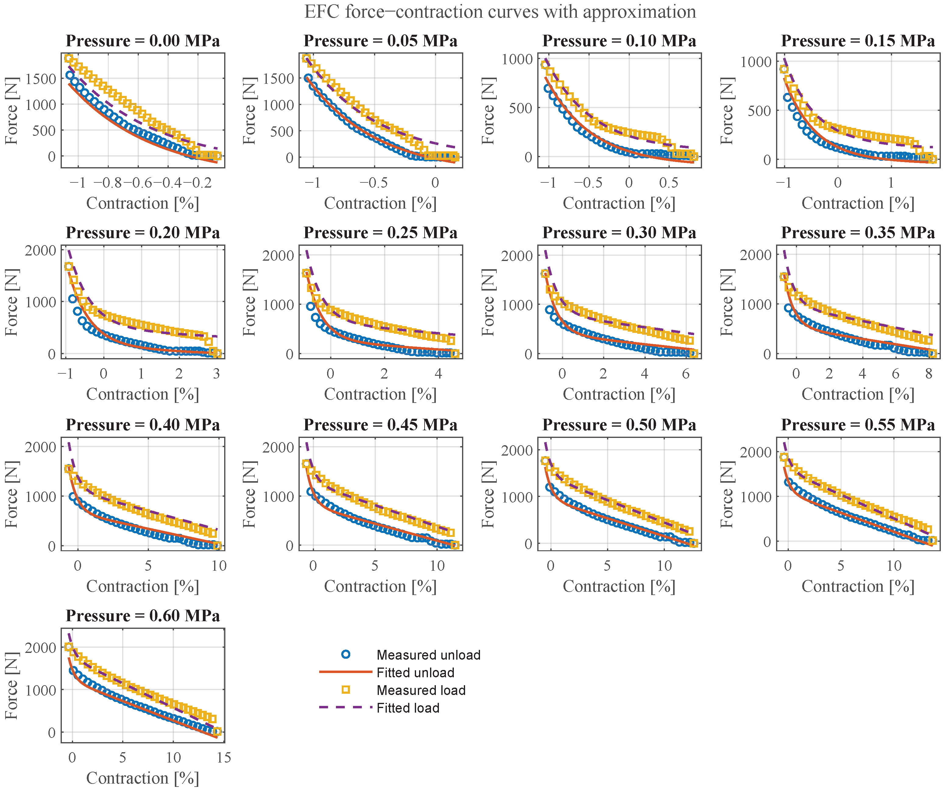
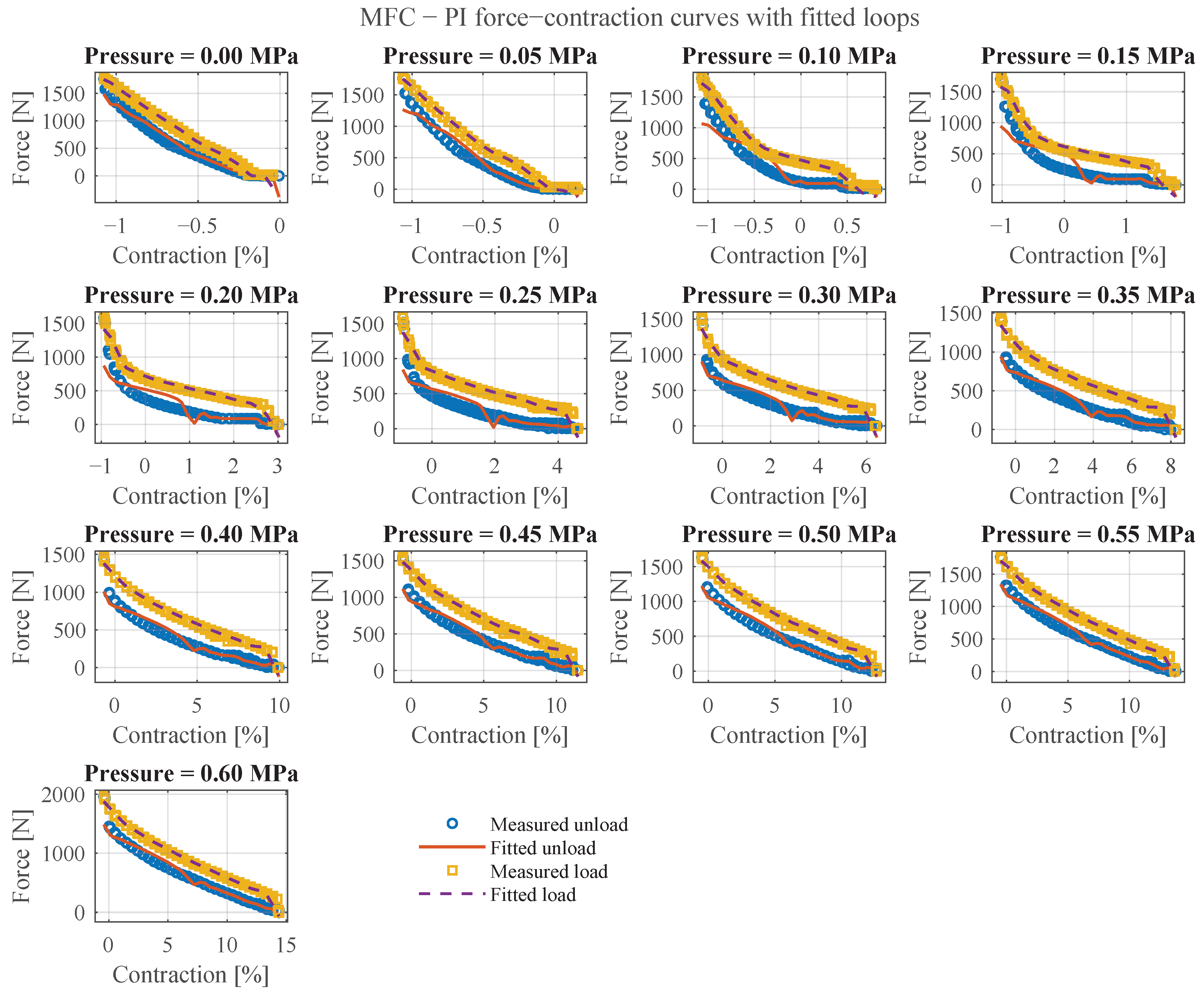
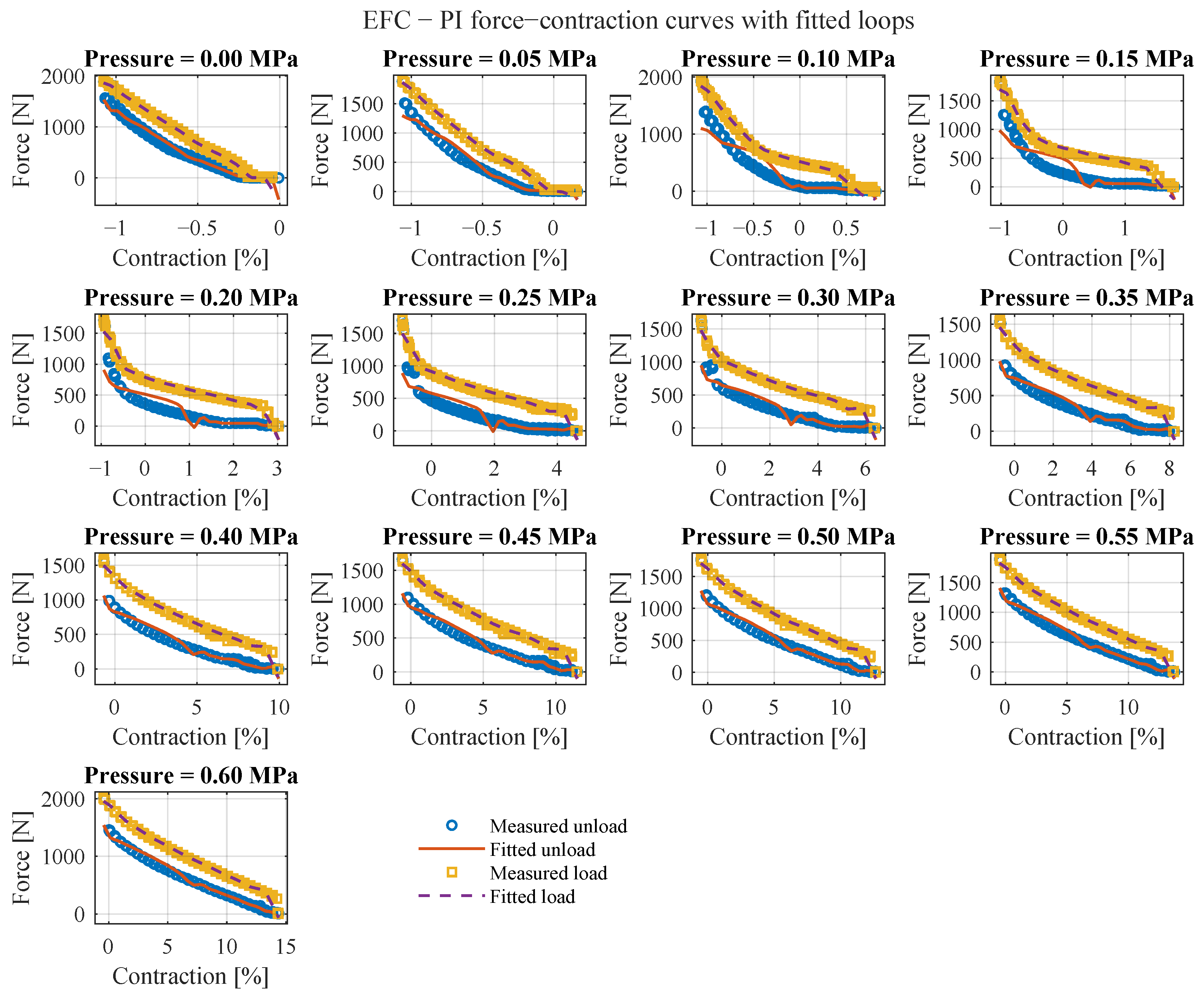
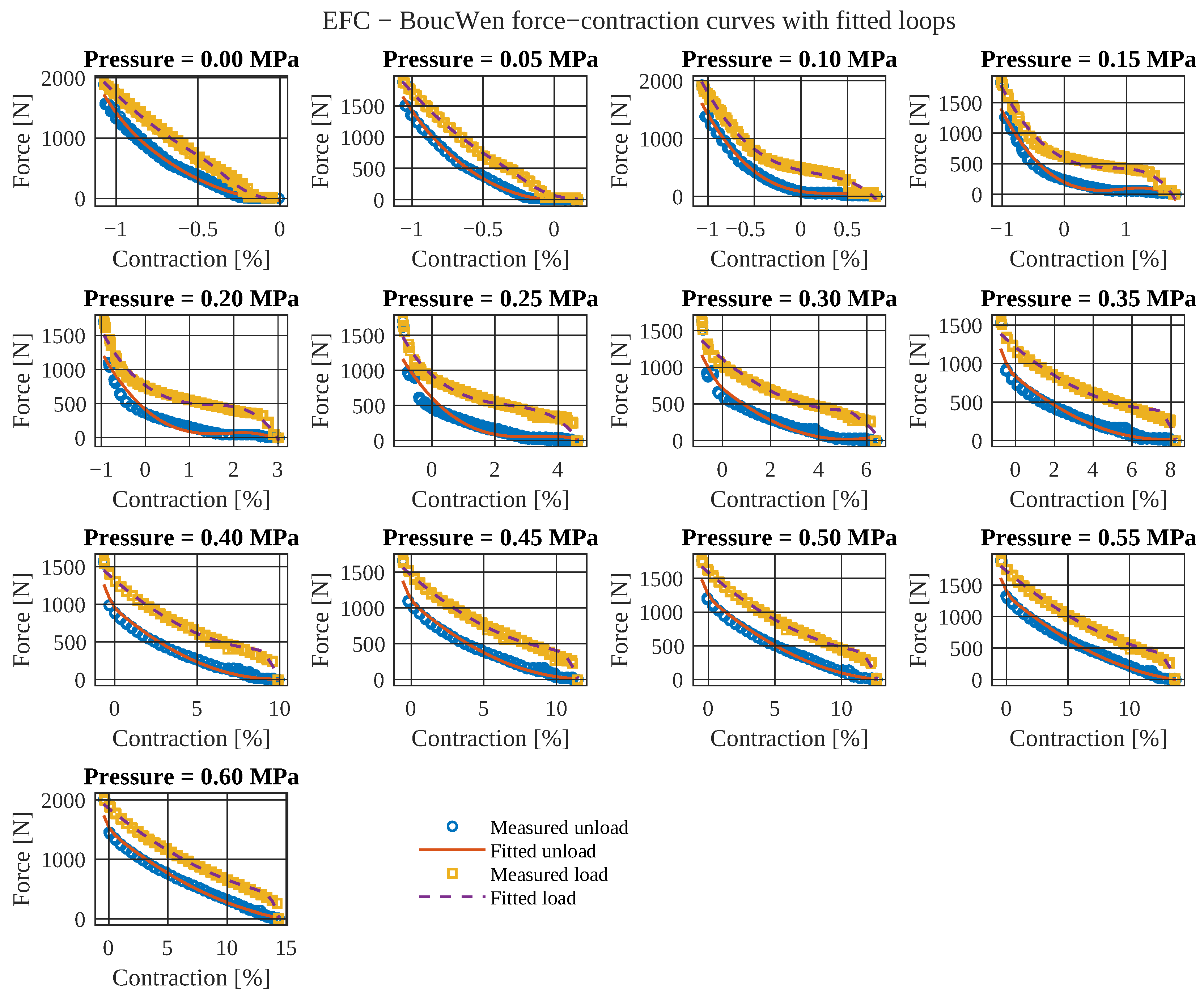
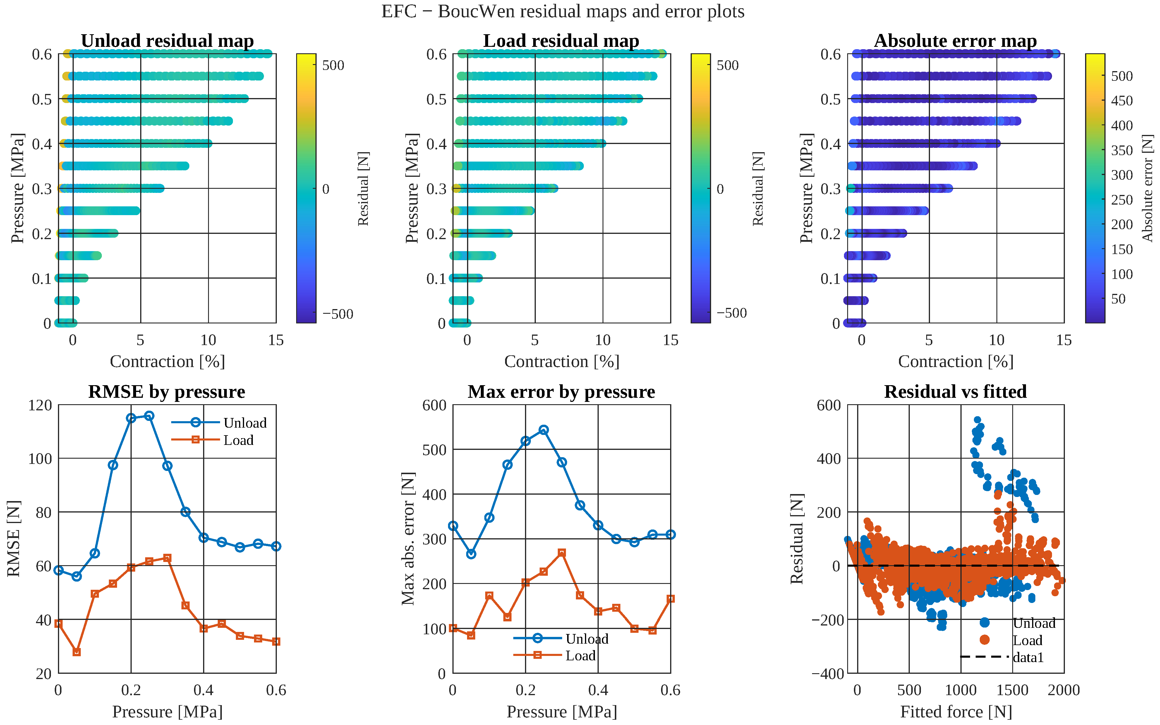
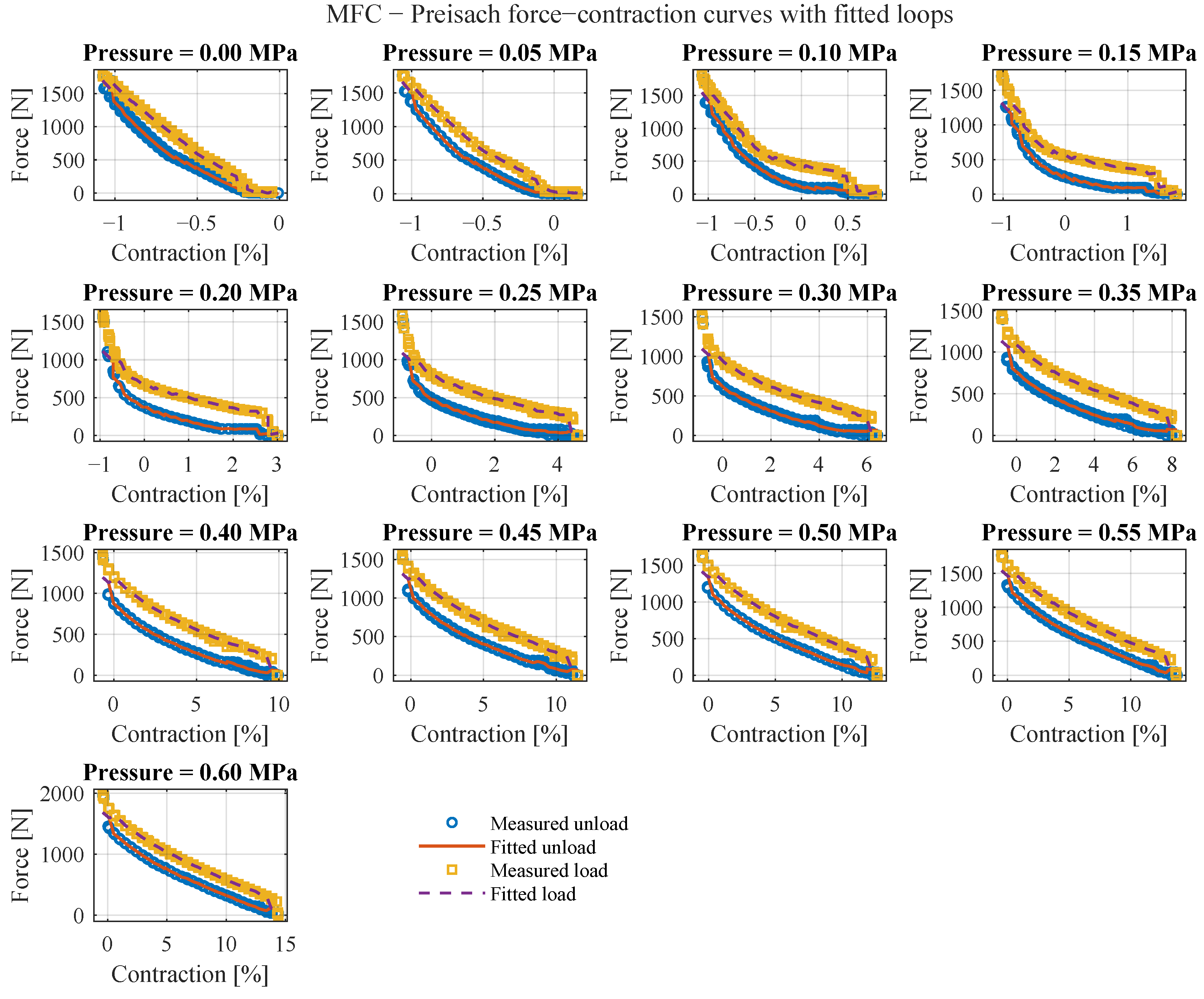
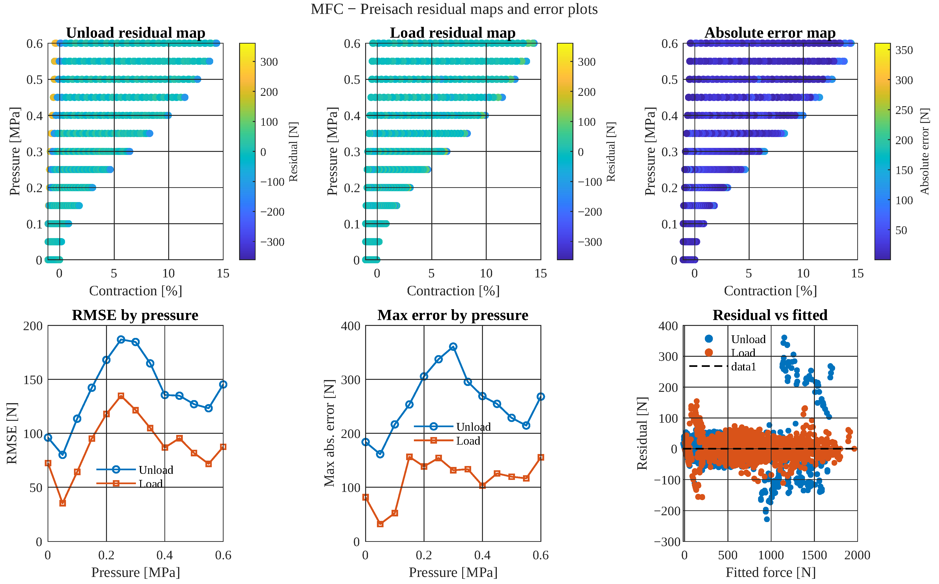
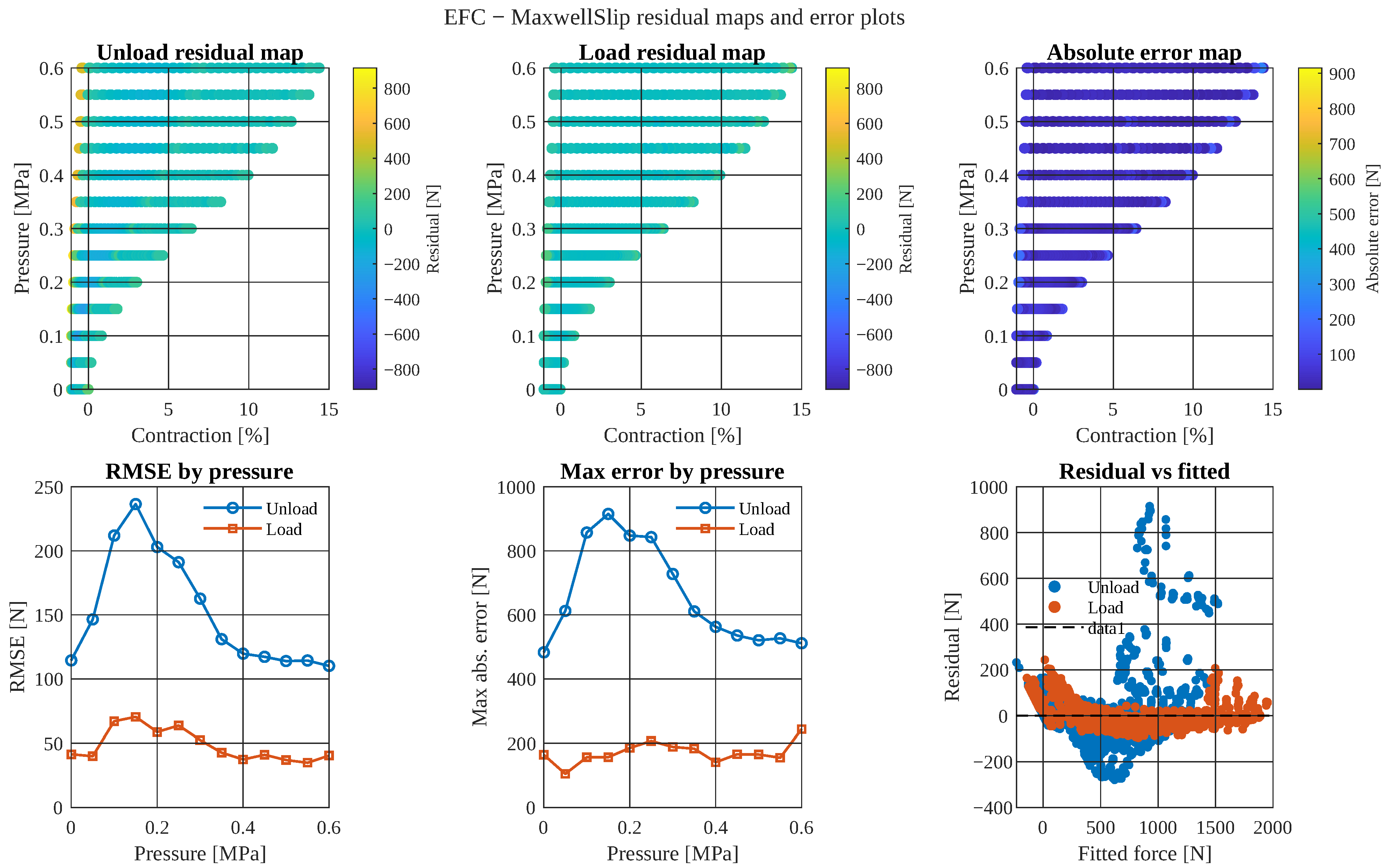
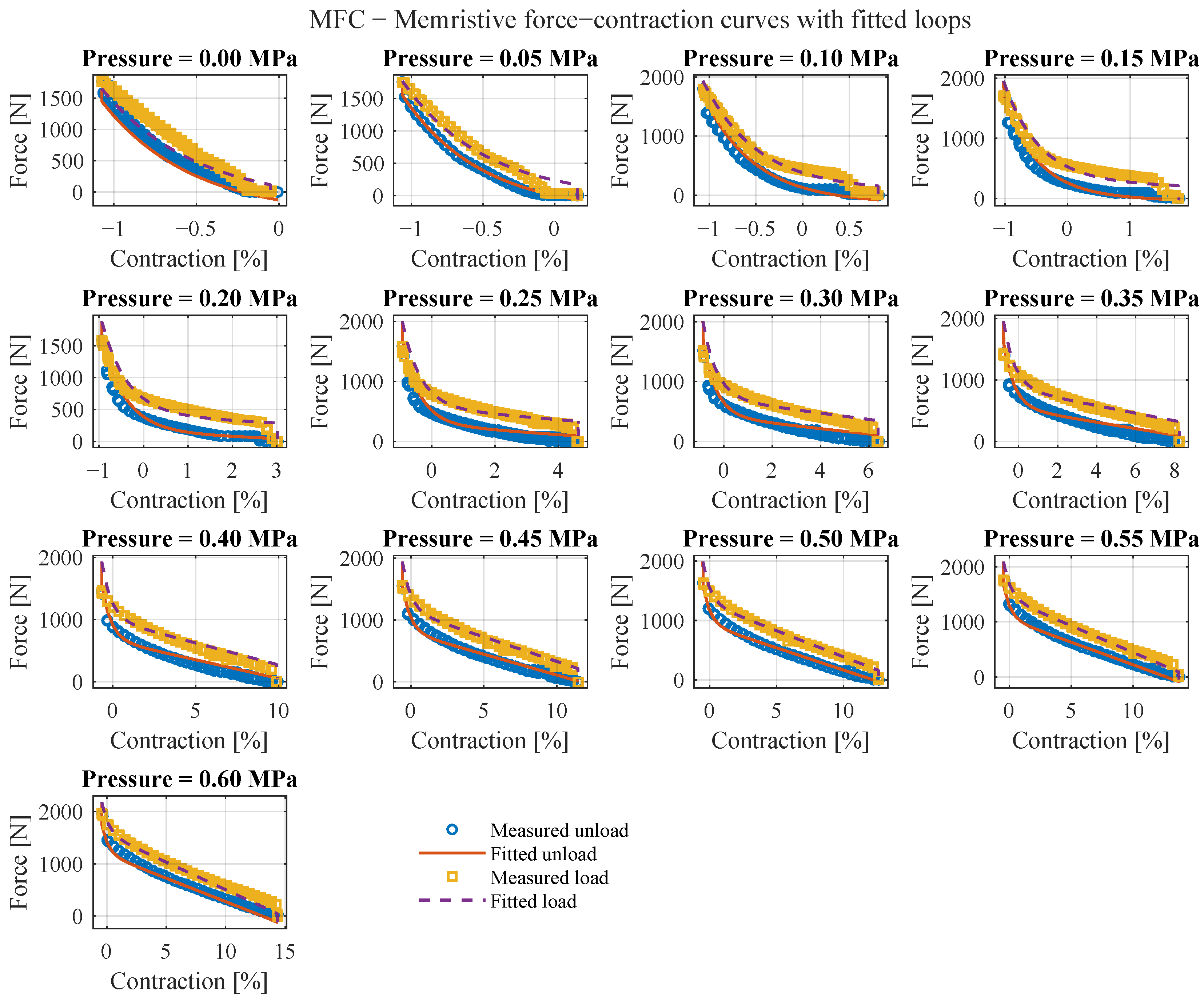
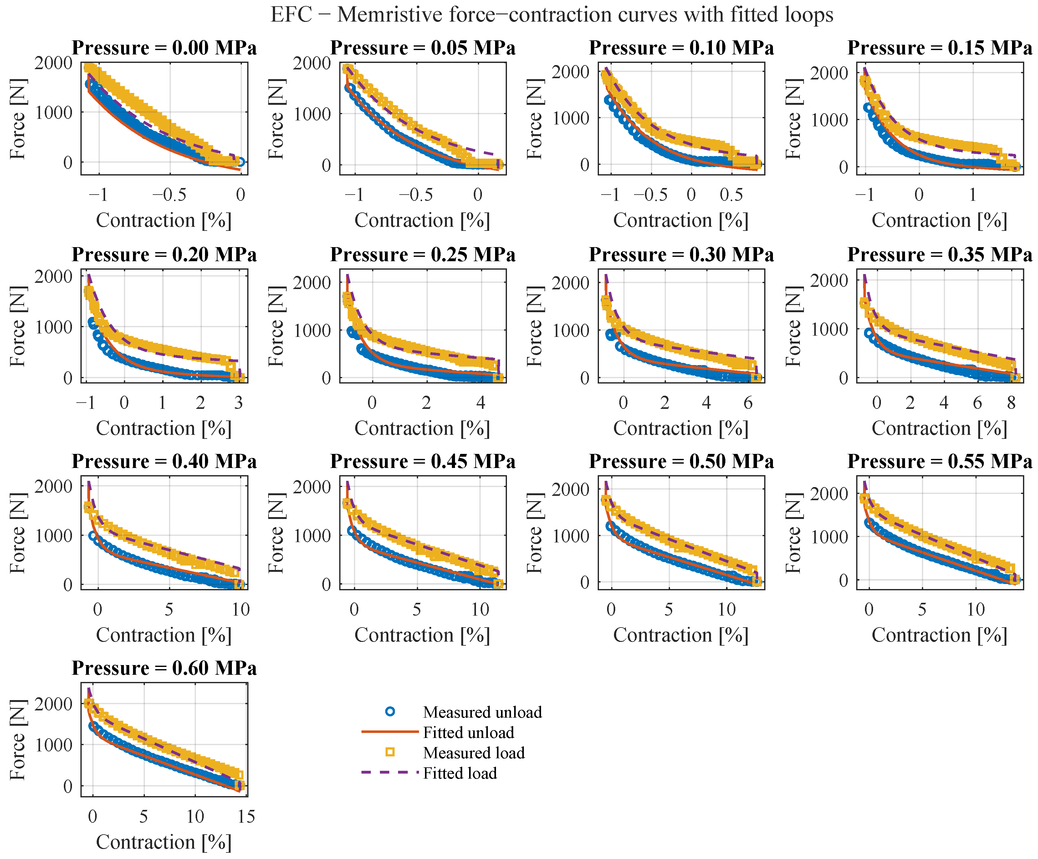
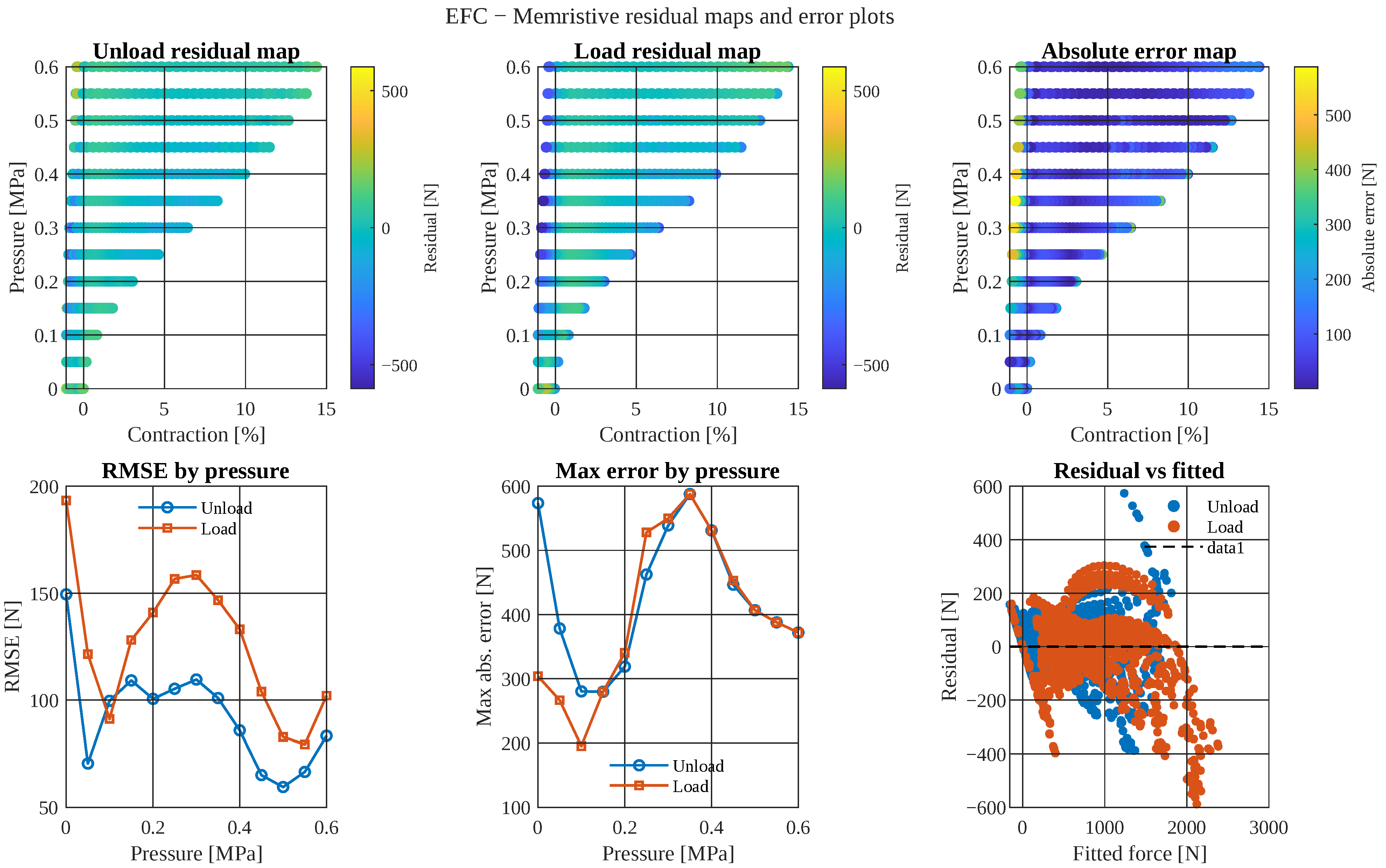
The corresponding coefficients were identified in the MATLAB Curve Fitter using the custom-equation option. The fitting method was nonlinear least squares, robustness was set to least absolute residuals (LAR), and the algorithm was trust-region. The parameters a 1 , a 2 , a 3 , a 4 , and a 5 were bounded during the fit as follows: 150 a 1 315 , 2 a 2 1 , 200 a 3 140 , 2500 a 4 3300 , and 500 a 5 0 . These bounds were imposed as practical identification constraints rather than as universal physical limits. Their role is to prevent numerically unstable or physically implausible branch-surface shapes during optimization. The intervals were selected from preliminary fitting trials, the scale of the measured force-pressure-contraction data, and the expected sign/magnitude behavior of the coefficients in the adopted Sárosi–Fabulya branch function. The identified values and their goodness of fit are listed in Table 2. Figure 3 and Figure 4 present the fit of the functions on the MFC and EFC data points, respectively. Figure 5 and Figure 6 show the goodness of the fit.

3.4. Identified Branch Equations

Substituting the coefficients from Table 2 into Equation (9) gives the four branch equations used in the current implementation:
F EFC u n l o a d ( ε , p ) = p + 283.5532 e 1.7535 ε 152.8966 ε p + 2719.0 p 444.4829
F EFC l o a d ( ε , p ) = p + 299.2673 e 1.7530 ε 189.3924 ε p + 3175.5 p 195.3742
F MFC u n l o a d ( ε , p ) = p + 253.8404 e 1.8403 ε 149.5208 ε p + 2591.3 p 383.4218
F MFC l o a d ( ε , p ) = p + 277.6454 e 1.7597 ε 175.9270 ε p + 2910.6 p 188.3115

4. Memristive-System-Based Hysteresis Model

4.1. Modeling Idea

A single-valued surface F ( ε , p ) cannot reproduce hysteresis because two different force values may correspond to the same ( ε , p ) pair depending on whether the actuator is on the loading or unloading path. To resolve this, the model uses the state-dependent branch mixture already introduced in Equation (6).
In that form, x = 0 corresponds to the unloading branch and x = 1 corresponds to the loading branch. Intermediate values allow a smooth transition if later datasets motivate gradual branch switching. In the current paper, the model is called memristive-system-based because the output force depends on both the present input pair ( ε , p ) and an internal state carrying branch memory.
Within this reduced formulation, the actuator is approximated as evolving between two experimentally identified quasi-static manifolds. The scalar state x is therefore the minimal memory variable required to distinguish which manifold is active. This role is narrower than in distributed-operator hysteresis models, because the branch geometry itself is supplied by the identified loading and unloading surfaces and the state variable is used only to select or blend between them.

4.2. State Update Law

The proposed hysteresis formulation combines the loading and unloading branch surfaces through a bounded internal state variable x n [ 0 , 1 ] , which represents the actuator’s branch memory at the nth sampled point. The estimated force is written as
F ^ n = x n F load ( ε n , p n ) + 1 x n F unload ( ε n , p n ) ,
where ε n and p n denote the measured contraction and pressure, respectively.
The state is updated in discrete time according to
x n + 1 = x n + α s n x n , 0 α 1 ,
where s n { 0 , 1 } is the branch indicator and α controls the transition sharpness between the unloading and loading surfaces. In the present implementation, s n = 0 corresponds to the unloading branch and s n = 1 corresponds to the loading branch. Accordingly, for 0 < α < 1 the internal state evolves gradually toward the active branch, whereas α = 1 corresponds to the hard-switching limit.
The use of the discrete-time update law is consistent with the scope of the present study. The model is identified and evaluated from sampled quasi-static experimental data, and the objective is hysteresis-loop reconstruction rather than continuous-time dynamic modeling or controller synthesis. Therefore, the proposed formulation is presented here as a discrete-time branch-memory model for the measured CPAM behavior.
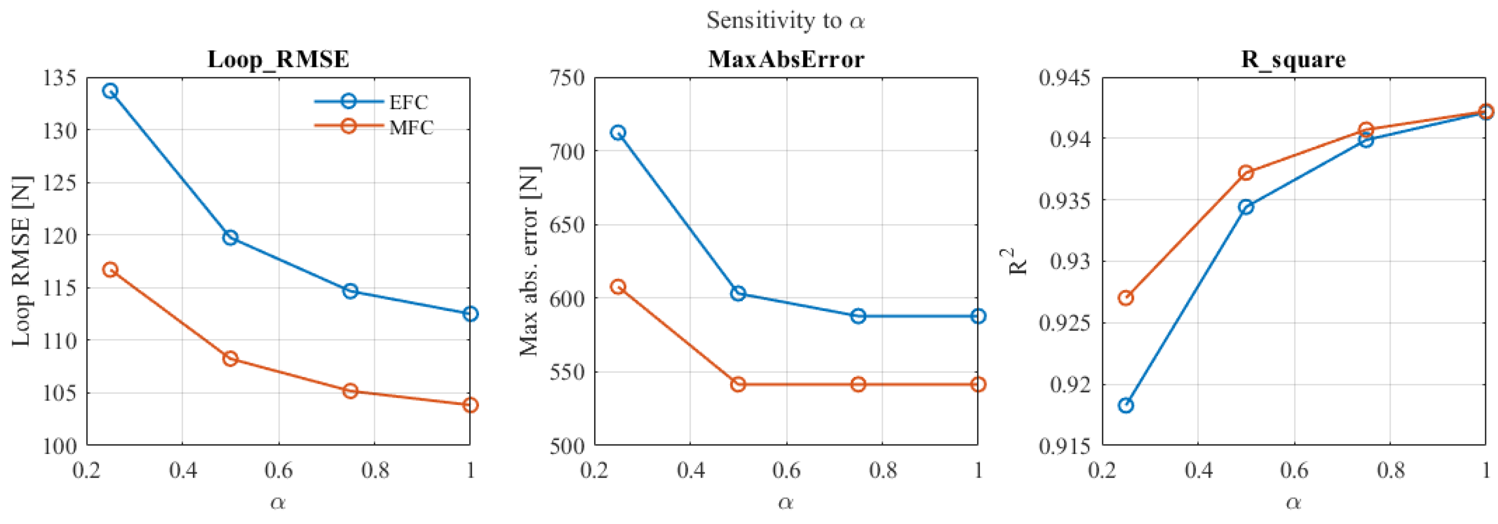
The parameter α was not fixed a priori. Instead, it was evaluated over a prescribed range during identification, and the best agreement with the measured quasi-static loops was obtained for α = 1 . Smaller values of α produced smoother transitions between the branch surfaces, but reduced the overall reconstruction accuracy on the available dataset. For this reason, the hard-switching case is retained in the present paper as the best-performing discrete-time setting for the investigated operating condition.
Since the update law in (15) is a convex combination of the previous state and the branch indicator, the interval x n [ 0 , 1 ] is forward invariant provided that the initial value satisfies x 0 [ 0 , 1 ] . The state therefore remains bounded throughout the loop reconstruction process.

4.3. Cycle Construction

For each pressure level, the measured hysteresis cycle is assembled from the branch data in the same order as the model evaluation:
1.
The unloading branch is ordered by increasing contraction.
2.
The loading branch is ordered by decreasing contraction.
3.
The turning point is included only once to avoid duplication.
The resulting cycle therefore contains
N = 32 + ( 32 1 ) = 63
points per pressure level when the turning point is shared. This matches the current evaluation logic in the MATLAB script.

4.4. Model Variants

Two variants are evaluated in the current manuscript:
  • Variant A: the EFC model generated by coupling F EFC u n l o a d and F EFC l o a d ;
  • Variant B: the MFC model generated by coupling F MFC u n l o a d and F MFC l o a d .
The purpose of retaining both variants is not to introduce two unrelated model classes, but to keep both force-contraction representations that were used in the MATLAB workflow.

5. Results and Discussion

The present manuscript is intentionally restricted to the 4 N / s dataset. Under that restriction, the primary confirmed results are structural rather than broad claims of dynamic generalization: the compact actuator has consistent loading and unloading branch surfaces for both EFC and MFC representations, and those surfaces can be coupled by a bounded internal state to reproduce a hysteretic force predictor in memristive-system form.

5.1. Branch-Surface Identification

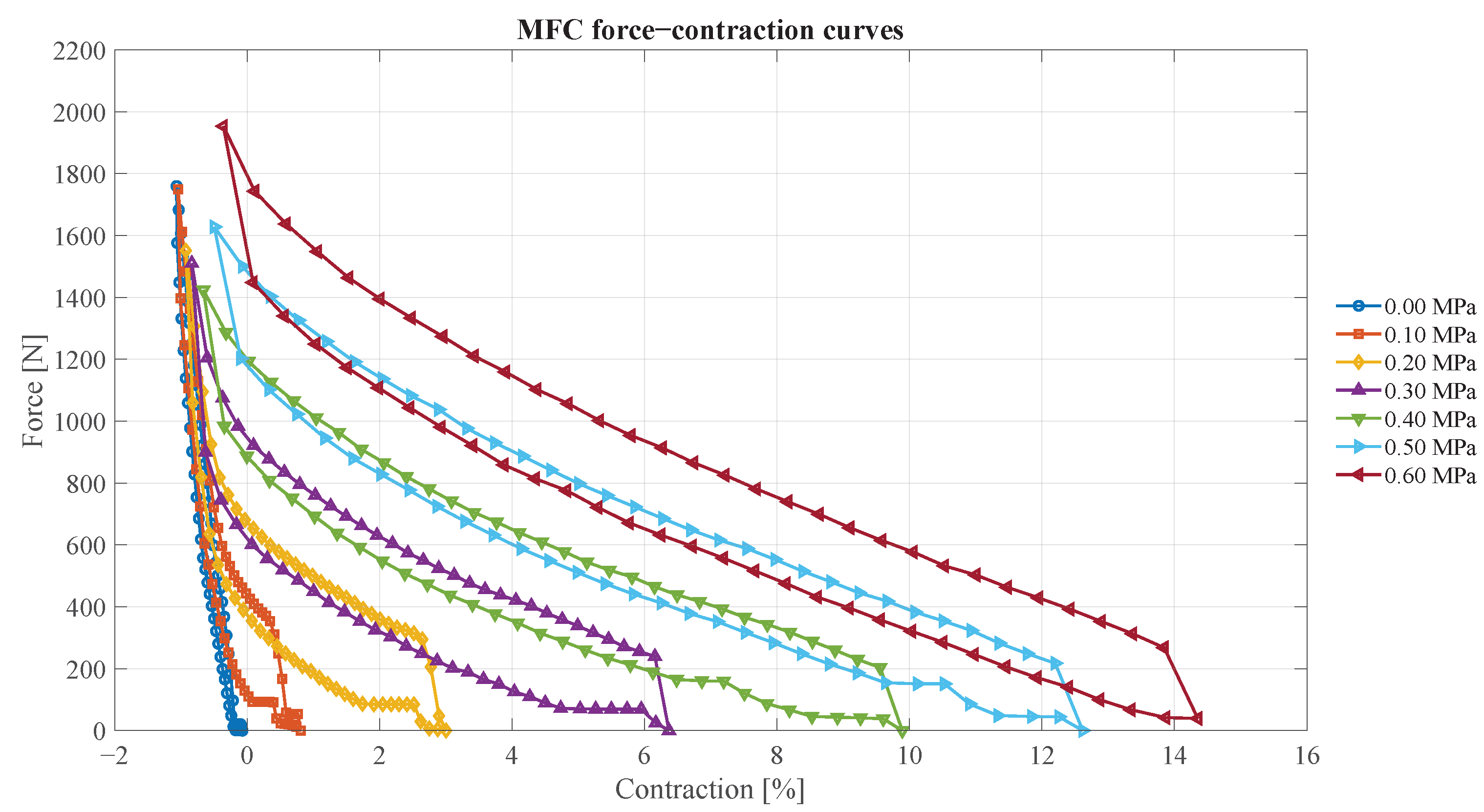
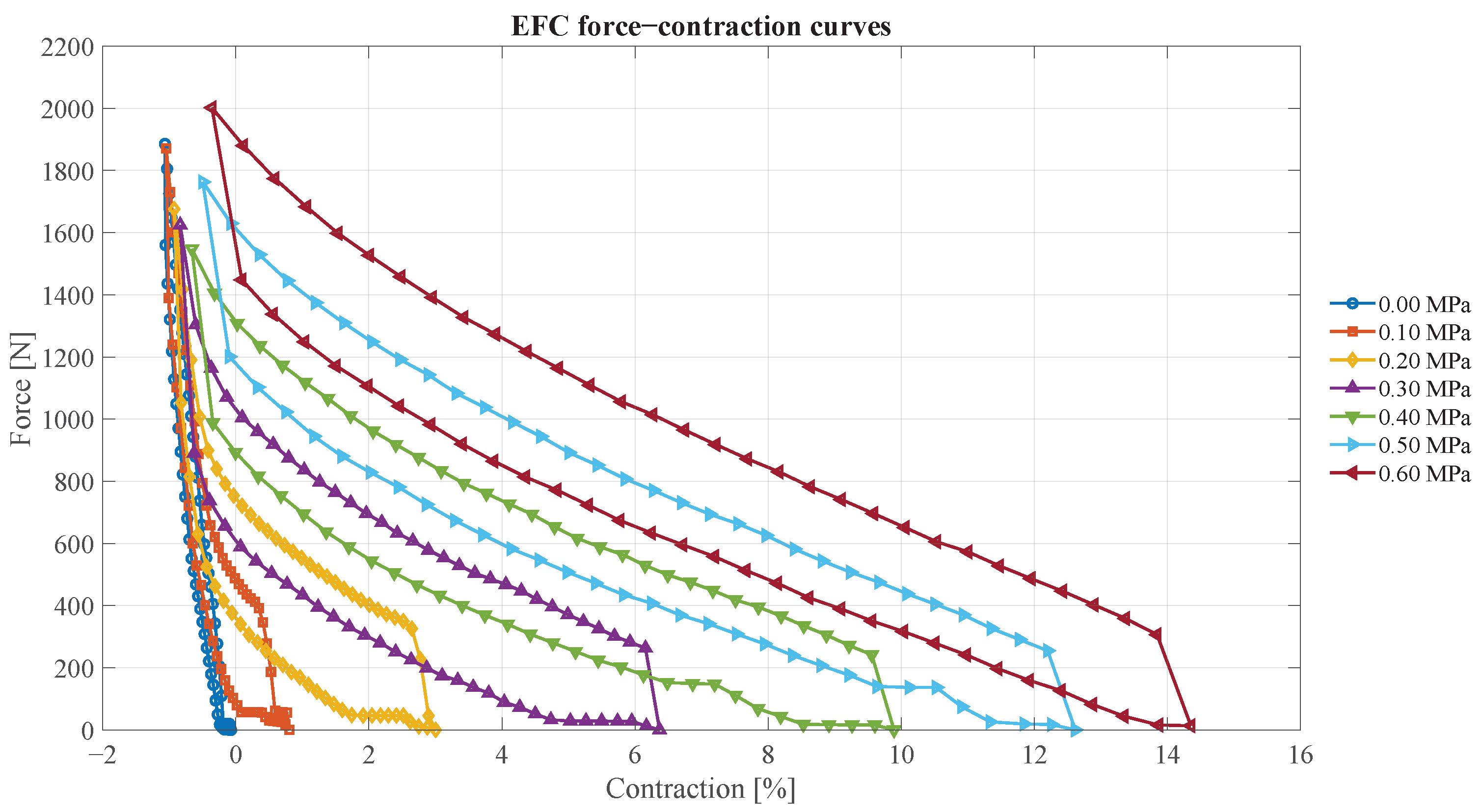
The first result is that the same five-parameter analytical form was sufficient for all four identified branches reported in Section 3. This is important because it keeps the modeling problem branch-dependent rather than model-family-dependent. At the same time, the current paper does not claim that the chosen Sárosi–Fabulya approximation is universally optimal among all possible branch regressors. Rather, it is retained here because it provides a low-parameter and interpretable surface for the available quasi-static dataset. The hysteresis representation does not require one functional form for unloading, another for loading, and yet another for a second force representation. Instead, the same analytical structure is preserved across all four identified surfaces. Figure 7 and Figure 8 show the MFC plots, while Figure 9 and Figure 10 show the corresponding EFC plots.
The branch coefficients also show directly that the actuator behavior is asymmetric. If the loading and unloading branches were identical, a single surface would have been sufficient and the internal memory state would be unnecessary. The need for separate loading and unloading equations is therefore already visible at the identification stage.

5.2. Quantified Hysteresis Asymmetry

The branch-wise plots show clear separation between loading and unloading, but that asymmetry should also be quantified explicitly. For consistency with our previous CPAM characterization study [20], the revised workflow will report a normalized hysteresis index (NHI) based on the enclosed loop area. For sampled data, the branch difference at pressure p is evaluated by subtracting the area under the branches and taking their absolute value as shown in Equation (17).
A h y s t e r e s i s ( p ) = A load ( p ) A unload ( p ) ,
A l o a d corresponds to the area under the load branch and A u n l o a d corresponds to the area under the unload branch. The corresponding branch area is approximated numerically by the trapezoidal rule, as seen in Equation (18)
A ( p ) i = 1 31 F i ( p ) + F i + 1 ( p ) 2 ε i + 1 ε i ,
The normalized hysteresis index is then calculated as shown in Equation (19).
NHI ( p ) = 100 % , A hysteresis ( p ) F max ( p ) ε 32 ε 1 ,
where F max ( p ) is the maximum measured force at the given pressure level. The quantity NHI ( p ) is therefore reported in percent as shown in Table 3.

5.3. Benchmarking Against Established Hysteresis Models

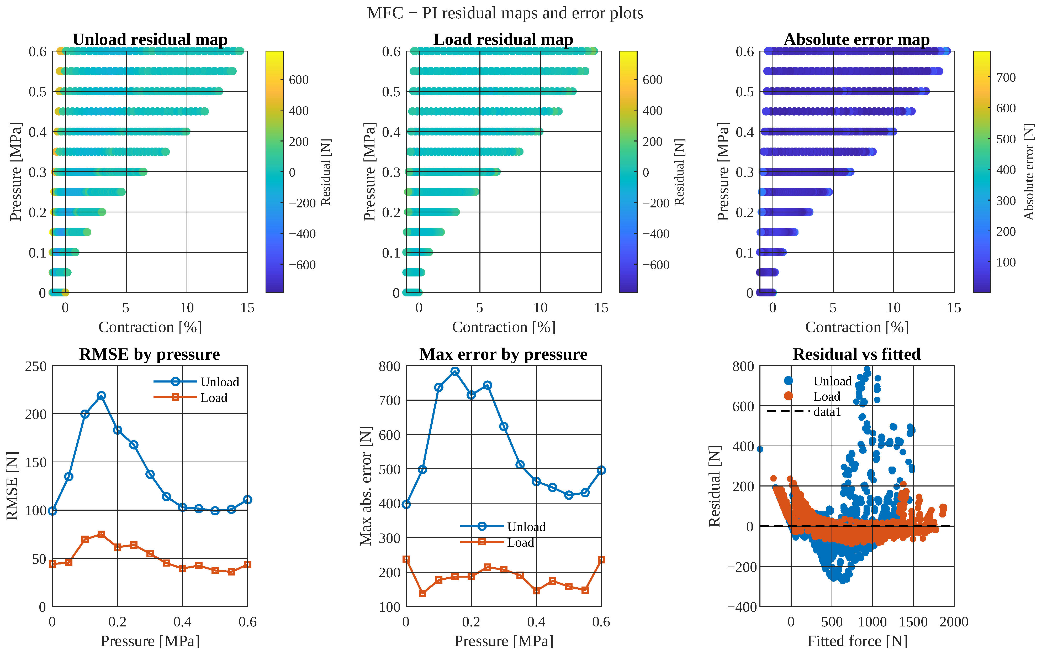
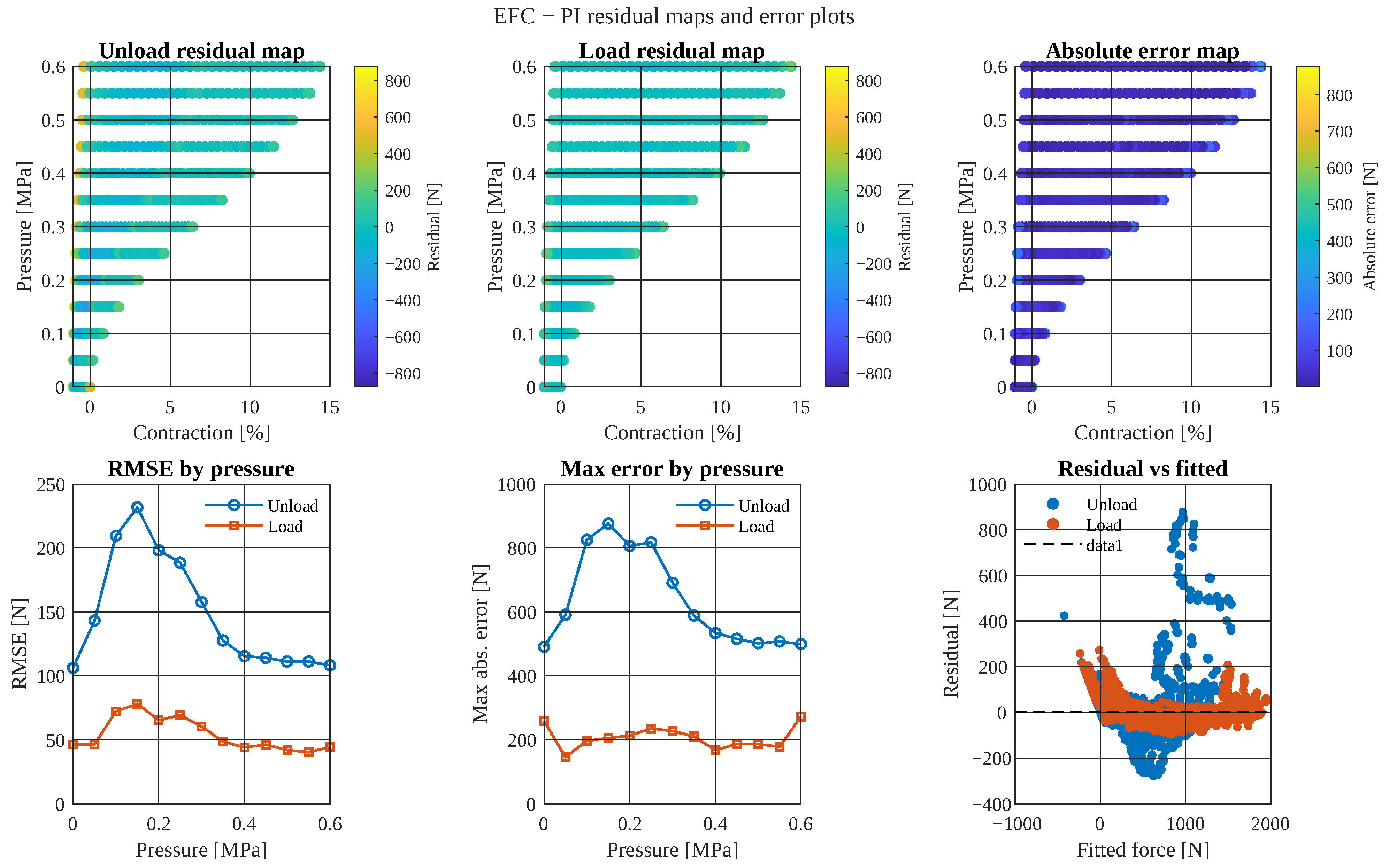
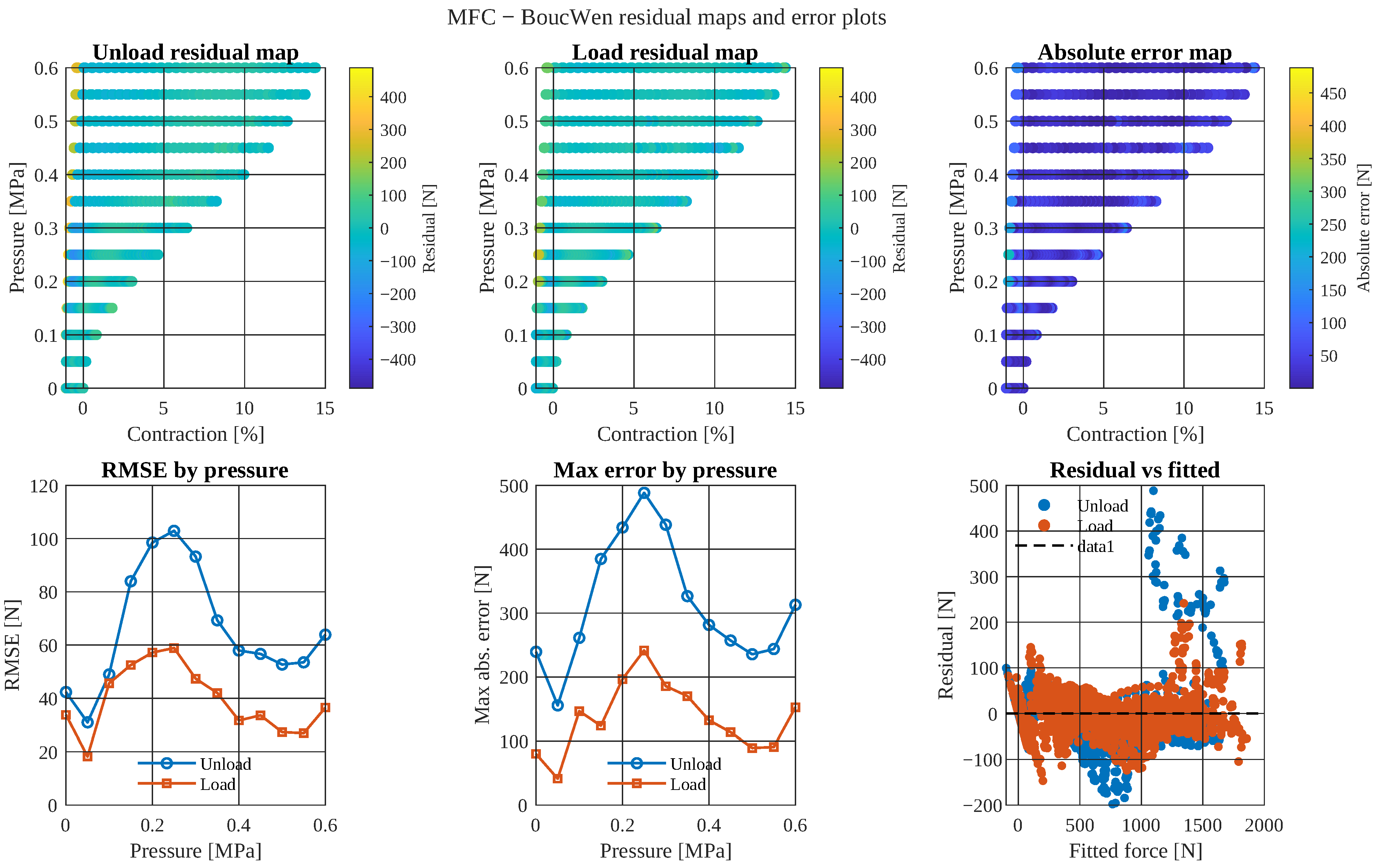
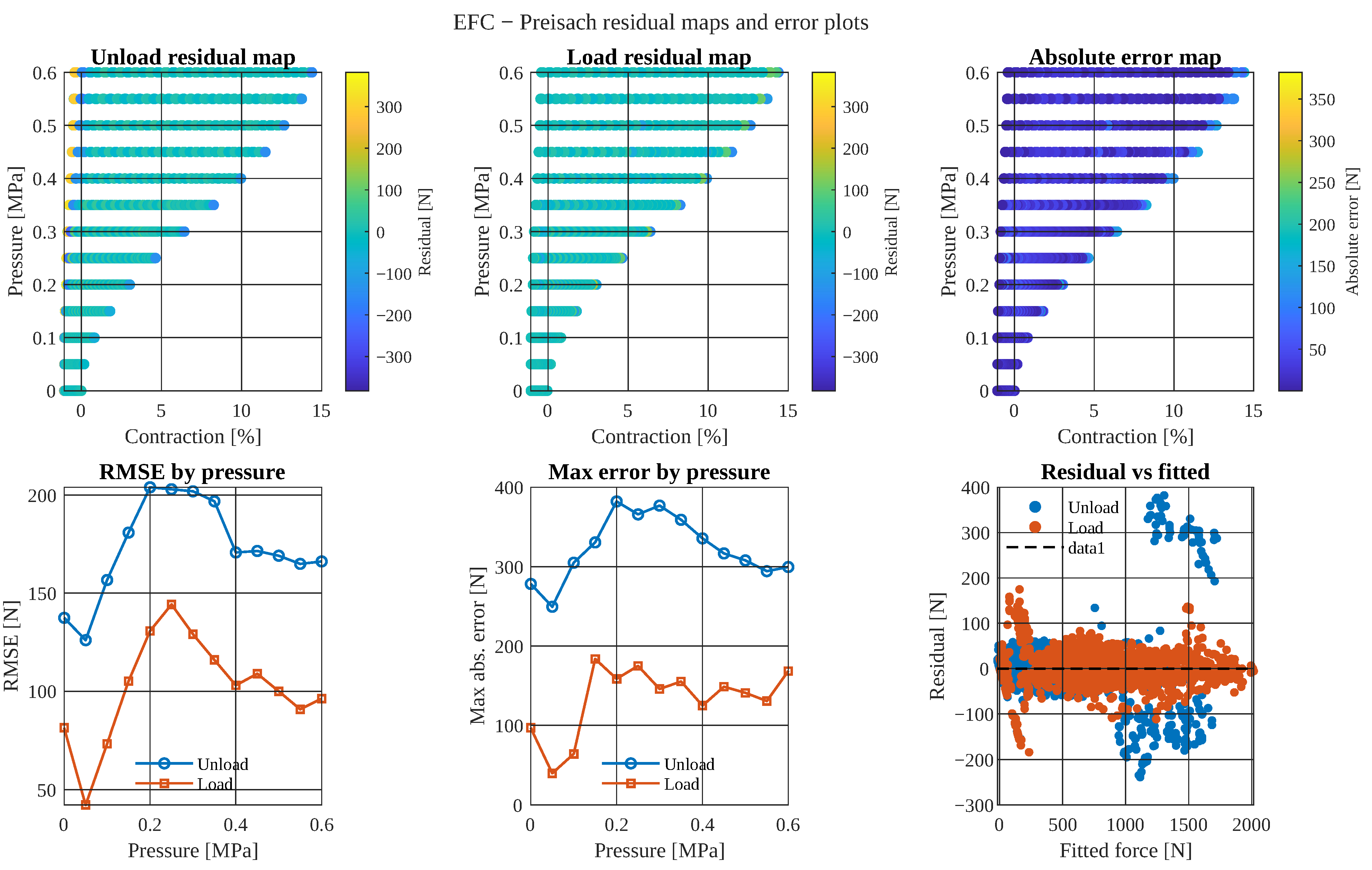
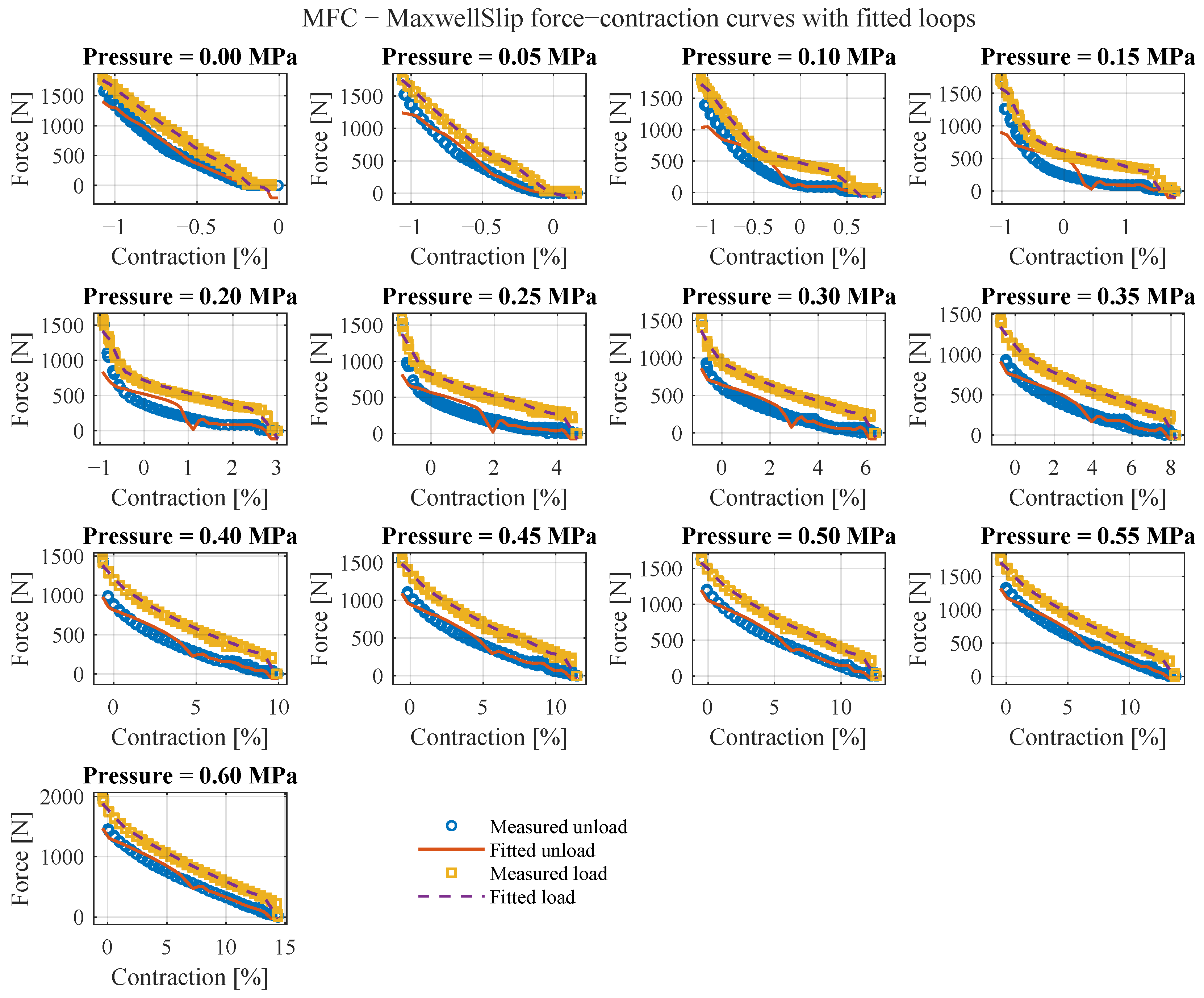
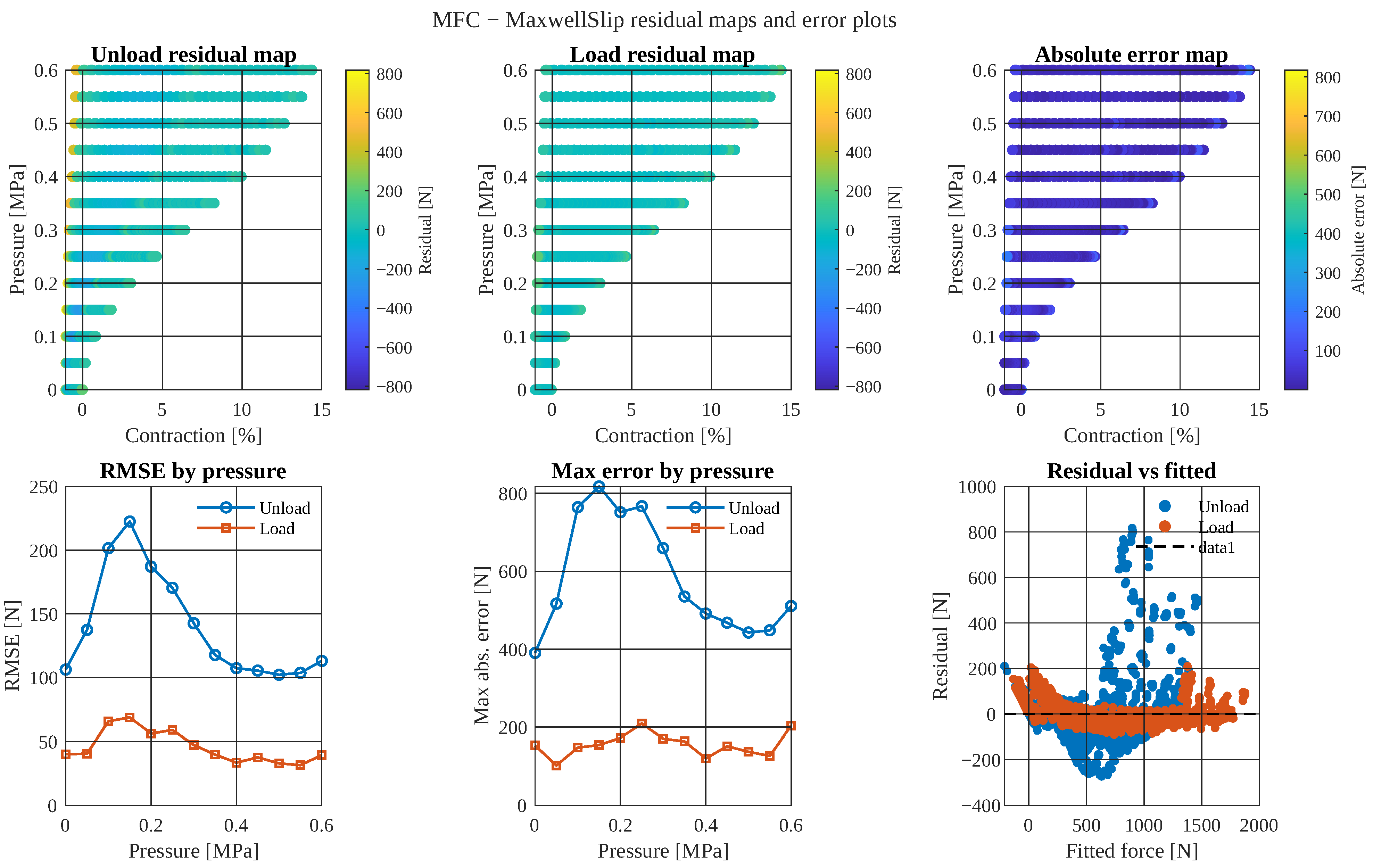
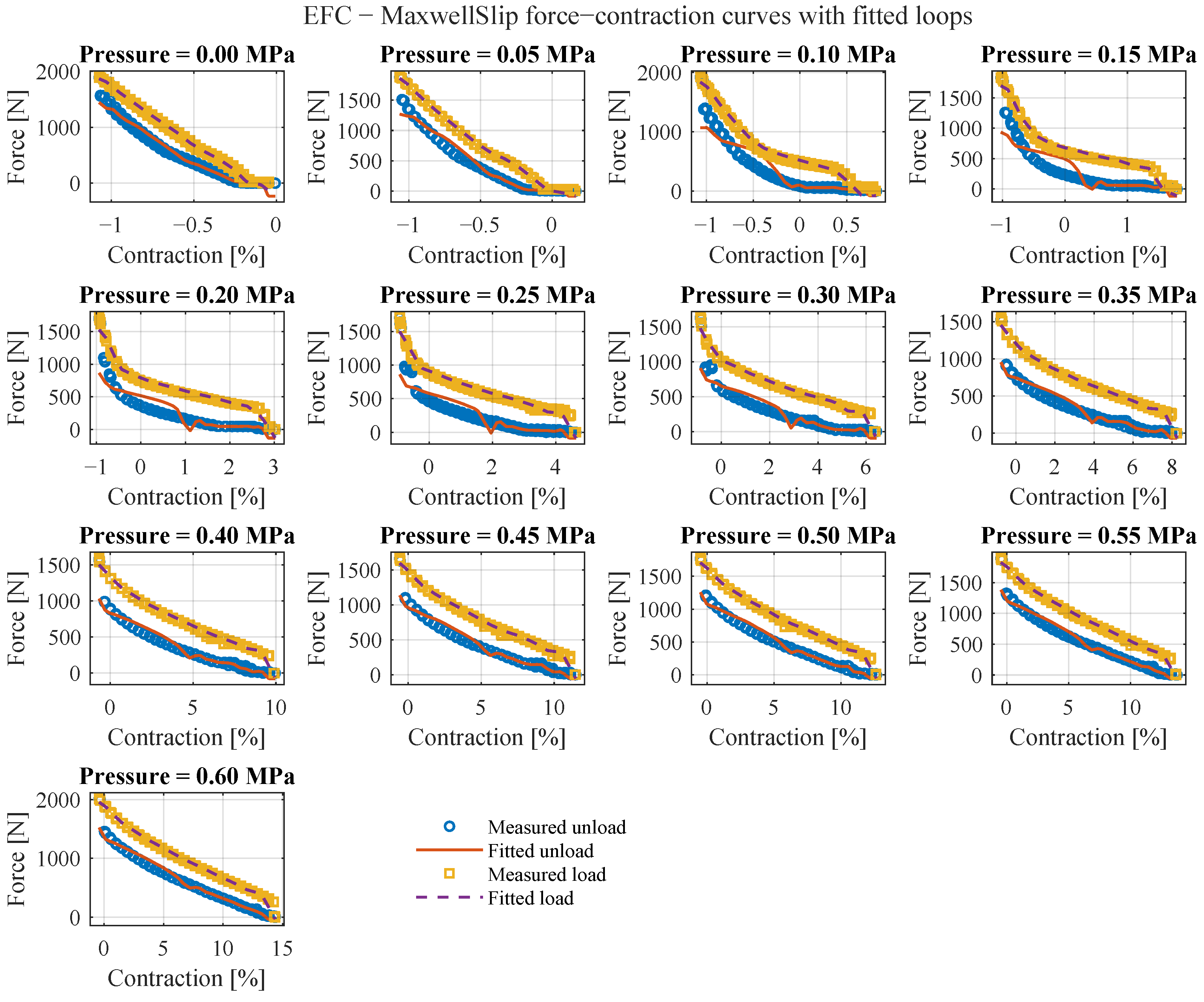
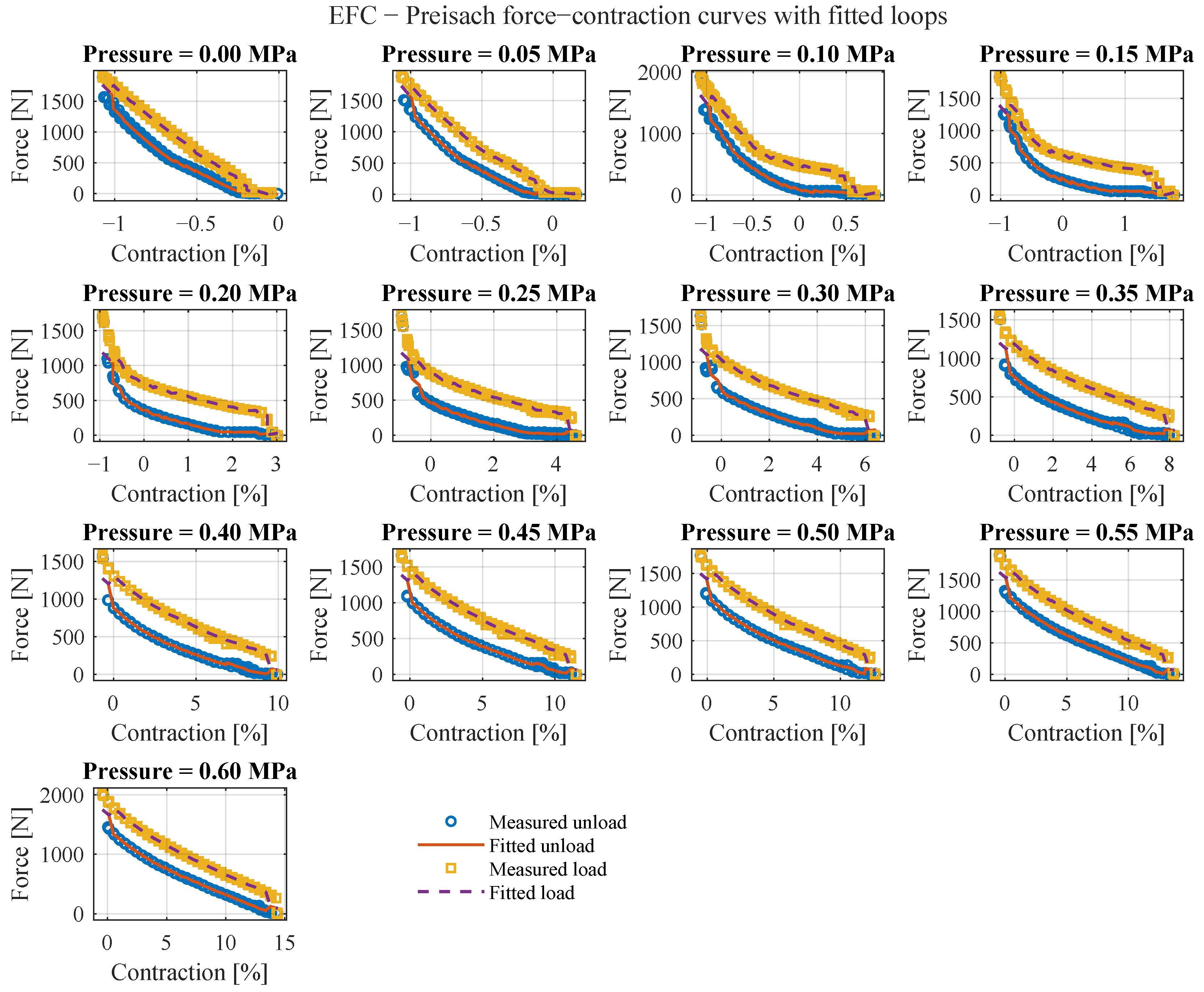
To position the proposed branch-memory formulation relative to established hysteresis-model families, additional benchmark models were evaluated on the same CPAM data sets. Specifically PI, discrete Preisach, Maxwell-slip, and sampled Bouc–Wen type models were fitted to the measured hysteresis loops of the EFC and MFC cases. In contrast to the proposed memristive formulation, which combines globally identified loading and unloading branch surfaces over the pressure-contraction domain, these benchmark models were used in their standard loop-modeling role, i.e., as hysteresis models for the measured force-contraction loops. The fitted models and their residuals are shown in Figure 11, Figure 12, Figure 13, Figure 14, Figure 15, Figure 16, Figure 17, Figure 18, Figure 19, Figure 20, Figure 21, Figure 22, Figure 23, Figure 24, Figure 25, Figure 26, Figure 27, Figure 28, Figure 29 and Figure 30. The coefficients for the models can be found in Appendix A. The resulting overall error metrics are summarized in Table 4.
For the EFC data set, the best reconstruction accuracy was obtained by the discrete Preisach model, with R 2 = 0.98774 and RMSE = 51.958 N , followed by the sampled Bouc–Wen-type model, with R 2 = 0.98123 and RMSE = 64.278 N . The proposed memristive model yielded R 2 = 0.94488 and RMSE = 110.160 N . For the MFC data set, the same ranking was observed: the discrete Preisach model provided the best fit, with R 2 = 0.99000 and RMSE = 43.364 N , followed by the sampled Bouc–Wen-type model, with R 2 = 0.98360 and RMSE = 55.541 N , whereas the proposed memristive model yielded R 2 = 0.94589 and RMSE = 100.88 N . The benchmark therefore shows that the proposed memristive formulation is not the most accurate loop-reconstruction model among the evaluated hysteresis-model families. In terms of average reconstruction accuracy, the Preisach and Bouc–Wen benchmarks outperform the proposed model on both EFC and MFC data. The PI and Maxwell-slip benchmarks also produce comparable or slightly better global R 2 values than the proposed model, although in the present implementation they exhibit larger maximum absolute errors than the memristive formulation. This indicates that the main weakness of the proposed approach is its lower average approximation accuracy rather than extreme localized mismatch alone. The comparison should also be interpreted in light of the different modeling objectives. The benchmark models are used here as loop-reconstruction models, whereas the proposed formulation is built from one analytical loading surface and one analytical unloading surface defined directly over the pressure–contraction domain, coupled through a single bounded internal memory variable. The proposed model should therefore be interpreted as a reduced-order global branch-memory representation rather than as a best-fit benchmark model. Its practical advantage is that the pressure dependence is embedded directly in the analytical branch surfaces, so the model remains available over the investigated quasi-static operating range without separate pressure-wise re-identification of the branch equations.

5.4. Memristive Coupling Interpretation

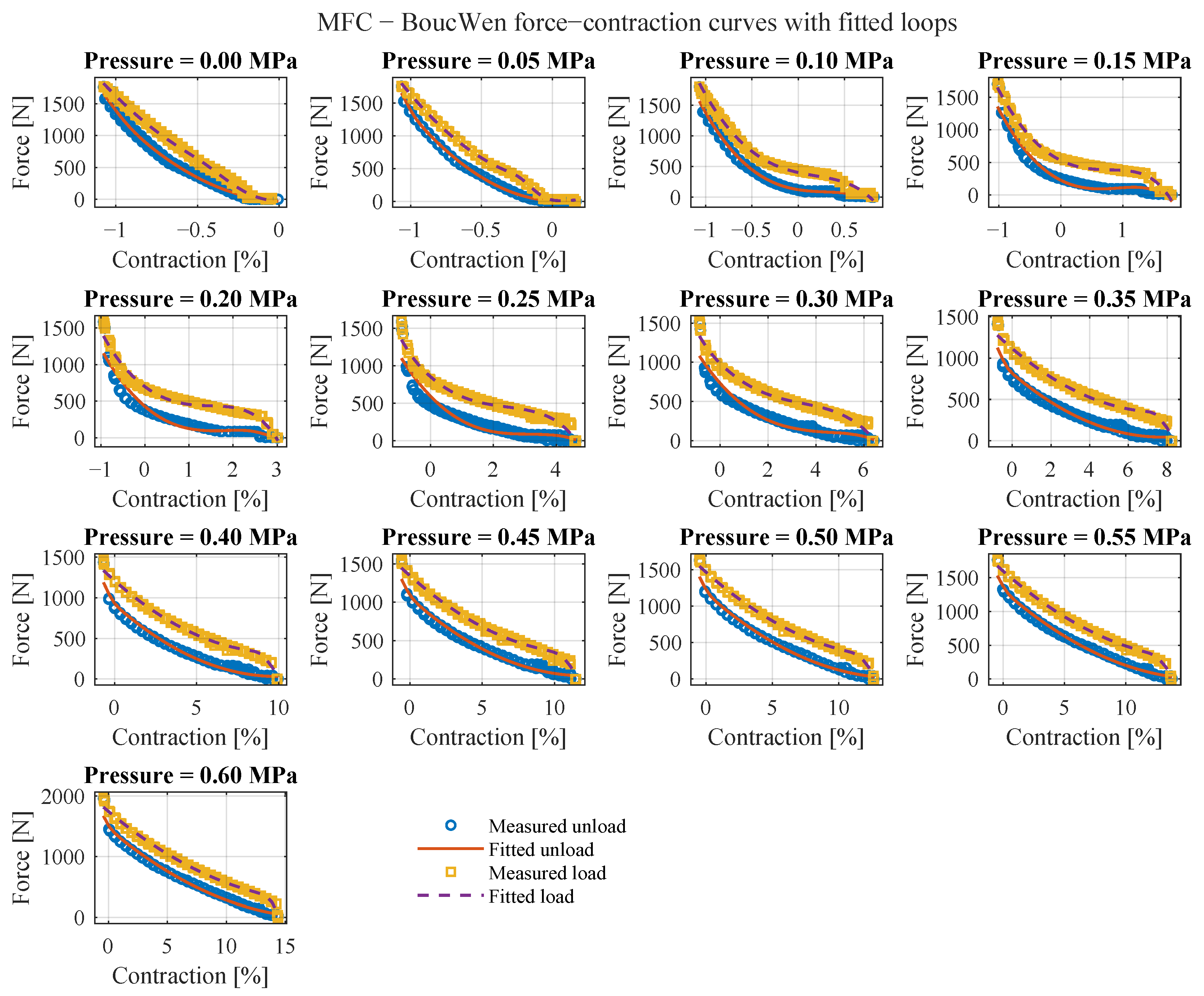
When the identified branch equations are embedded in Equation (6), the resulting predictor becomes a low-order hysteresis model with explicit branch memory. In the current implementation, α = 1 reduces the update law to a hard switch between the active branches. Even with that simplification, the model is useful because it ties the measured branch structure and the branch-selection logic into one state-dependent expression. The same state formulation can, in principle, also support smoother blending for 0 < α < 1 if later datasets justify it. The model’s sensitivity to α has been evaluated for values 0.25, 0.5, 0.75 and 1, the results of which are presented in Figure 31. Figure 3 and Figure 4 compare the fitted branch surfaces against the measured data for the MFC and EFC representations, while Figure 27 and Figure 29 show the corresponding memristive loop reconstructions.
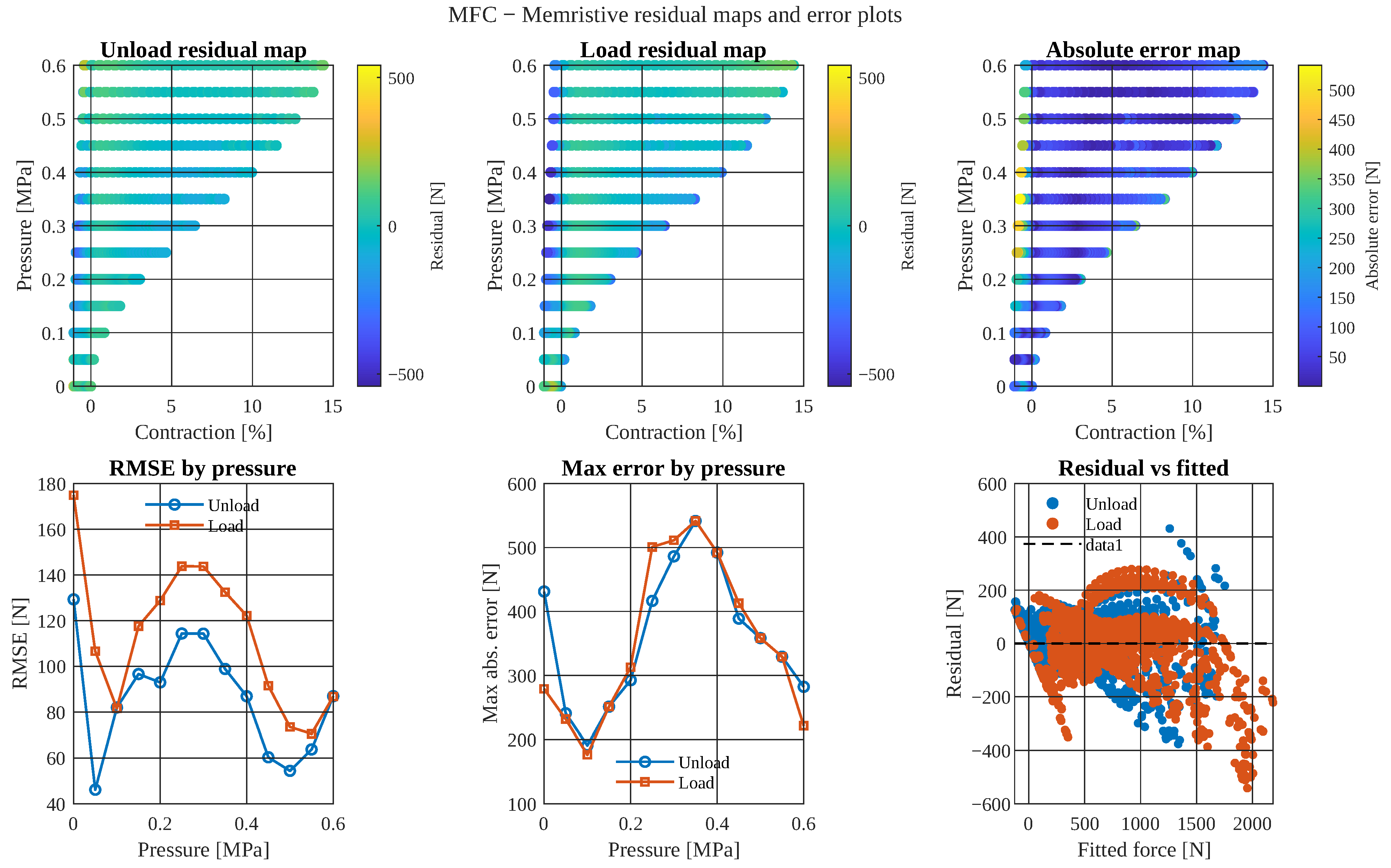
The drop from the branch-wise fit metrics in Table 2 to the loop-level metrics in Table 4 is expected. Each loading or unloading surface is fitted only to data from a single branch, so the fit quality is highest away from the reversal region. The full hysteresis predictor, however, must also pass through the change-of-direction region where the active description switches between two separately fitted functions. That transition region is therefore the least accurate part of the overall reconstruction, because it is governed by the crossover between the branch functions rather than by the interior of either well-fitted branch alone.
This point matters for the modeling claim of the paper. The contribution is not that the actuator behaves like an ideal electrical memristor. The contribution is that the hysteretic force response can be written in a generalized memristive-system form, in which the predicted output depends on both the present operating variables and an internal state carrying branch history.

5.5. Transition-Region and Spatial Residual Analysis

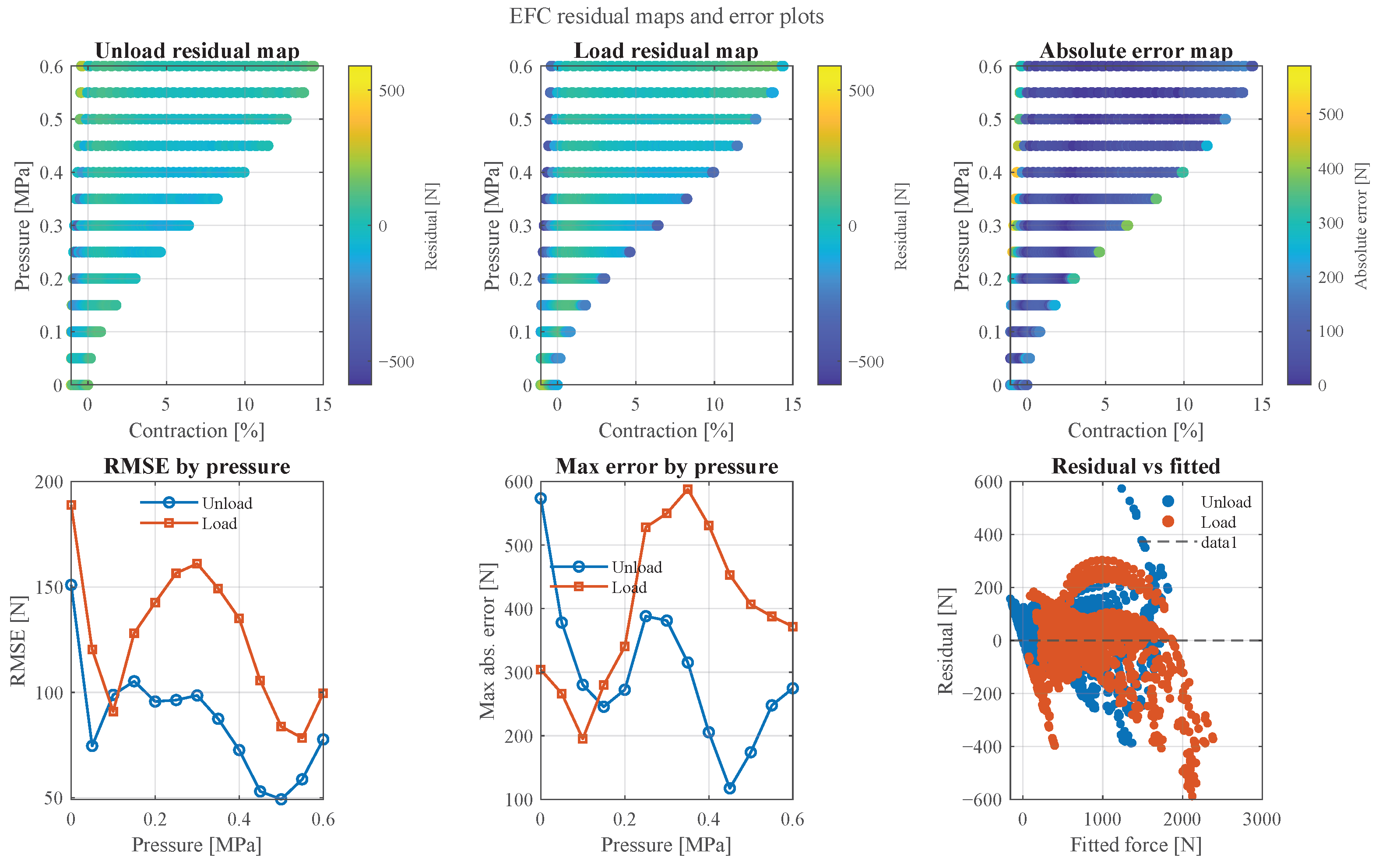
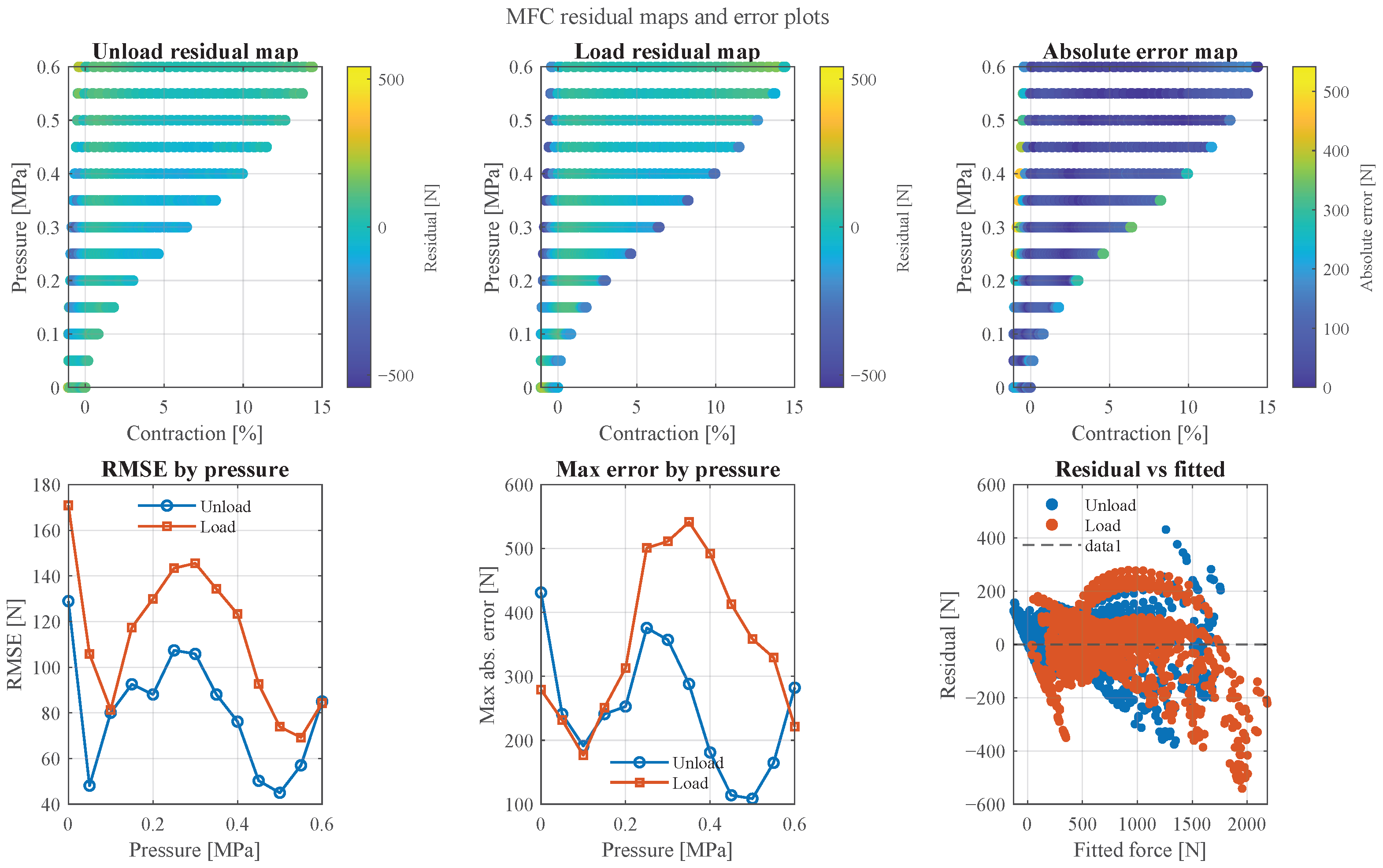
The loop-level metrics in Table 4 are aggregate indicators and do not show where the mismatch is concentrated. For the present model, the most likely error concentration is the loading/unloading reversal zone, because that is where the predictor crosses between two separately fitted branch surfaces. Examining the absolute error map of Figure 28 and Figure 30 we can observe that the greatest errors accumulate in the endpoints.

5.6. Current Validation Scope

The presented article is deliberately narrowed to only the quasi-static 4 N / s dataset, and the reported state law is branch-indicator driven rather than fully dynamic. The model should therefore be interpreted as a low-order phenomenological hysteresis representation at one operating rate. It does not yet support claims of multi-rate generalization or experimental validation of continuous dynamic state evolution.
No closed-loop controller is implemented in the present paper. The practical implication for control is therefore preparatory rather than demonstrative: the model provides a low-order hysteresis block that could later be embedded in feedforward compensation, force estimation, or control-oriented state-space formulations, but no tracking-performance improvement is claimed here.
Future work should extend the measurements to additional force-change rates and dynamic operating conditions and should then identify the continuous-time transition law directly from those richer datasets.

5.7. Strengths and Limitations

The main strength of the proposed formulation is its low structural complexity. It preserves the distinct loading and unloading force surfaces while introducing only one additional internal state. It is therefore more transparent than distributed-operator or many-element friction models and easier to align with the measured branch structure of the experiment.
The main limitations are equally clear. First, only one force-change rate is used, so rate robustness is not established. Second, the present state update is effectively instantaneous because α = 1, so the reported implementation should be interpreted as a discrete-time hard-switching branch-memory model under the tested quasi-static conditions. Third, the identified equations are phenomenological rather than uniquely mechanistic, so their coefficients should not be overinterpreted as direct estimates of braid friction, bladder elasticity, or end-effect deformation. Fourth, the available identification dataset is limited and the nominal branch surfaces are based on median-reduced repeated measurements; this reduces outlier sensitivity but may also conceal part of the cycle-to-cycle variability if not complemented by explicit uncertainty analysis. Fifth, the largest reconstruction errors occur near branch reversal, where the model crosses between two separately fitted branch surfaces. That transition region requires denser dedicated measurements and should be analyzed explicitly by residual maps, local uncertainty estimates, and smoother-transition identification. Finally, the low-order structure of the model makes it potentially attractive for future model-based compensation, but the present paper does not include closed-loop controller integration or tracking validation and therefore should not be interpreted as a demonstrated control-performance study.

6. Conclusions

This paper presents a low-order hysteresis model for a compact pneumatic artificial muscle using a memristive-system-based branch-coupling framework. Separate loading and unloading force surfaces were identified from force-contraction-pressure data recorded at a force-change rate of 4 N / s , and a bounded internal state formulation was used to combine those surfaces into a single hysteretic predictor.
The resulting manuscript supports a specific claim. At the fixed operating condition investigated here, branch-specific Sárosi–Fabulya surfaces can be embedded in a generalized memristive-system form and used to reconstruct hysteretic force behavior while retaining explicit mechanical variables. In the reported implementation, the state law is used in its hard-switching form with α = 1. The present implementation should therefore be read as a discrete-time quasi-static phenomenological model with branch memory, not as a continuous-time dynamic model and not as a demonstrated closed-loop control solution.

Author Contributions

Conceptualization, S.C.; methodology, S.C.; software, S.C.; validation, S.C.; formal analysis, S.C. and J.S.; investigation, S.C.; resources, J.S.; data curation, S.C.; writing—original draft preparation, S.C.; writing—review and editing, S.C. and J.S.; visualization, S.C.; supervision, J.S.; project administration, J.S.; funding acquisition, J.S. All authors have read and agreed to the published version of the manuscript.

Funding

This research received no external funding.

Institutional Review Board Statement

Not applicable.

Informed Consent Statement

Not applicable.

Data Availability Statement

Dataset available on request from authors.

Conflicts of Interest

The authors declare no conflicts of interest.

Appendix A. Compact Parameter Presentation for the Identified Models

The appendix avoids page-long coefficient dumps. The two operator-based models are summarized by coefficient heatmaps with rows corresponding to pressure levels and columns corresponding to coefficient indices. Bouc–Wen and branch-memory parameters are reported in compact tables because they are naturally low dimensional.
For the Prandtl–Ishlinskii and Maxwell-slip models, the common threshold vector is
r j = 0.04 j , j = 1 , , 24 .
For the Preisach model, the common relay lattice is
G = { ( α , β ) : α , β { 0 , 1 15 , 2 15 , , 1 } , β α } .
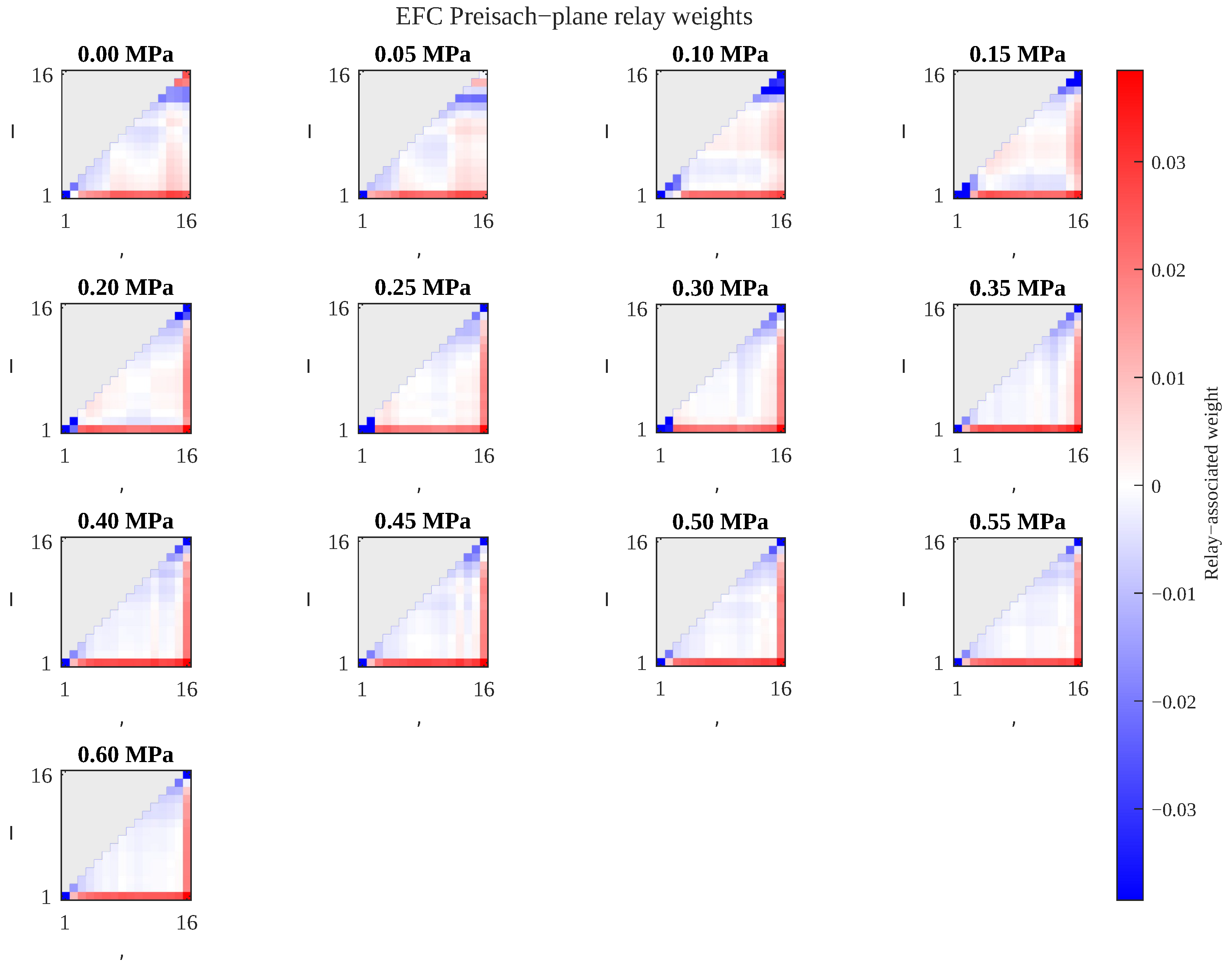
The Preisach-plane figures visualize only the relay-associated entries on this lattice.

Appendix A.1. EFC Dataset

Appendix A.1.1. Prandtl–Ishlinskii and Maxwell-Slip Representations
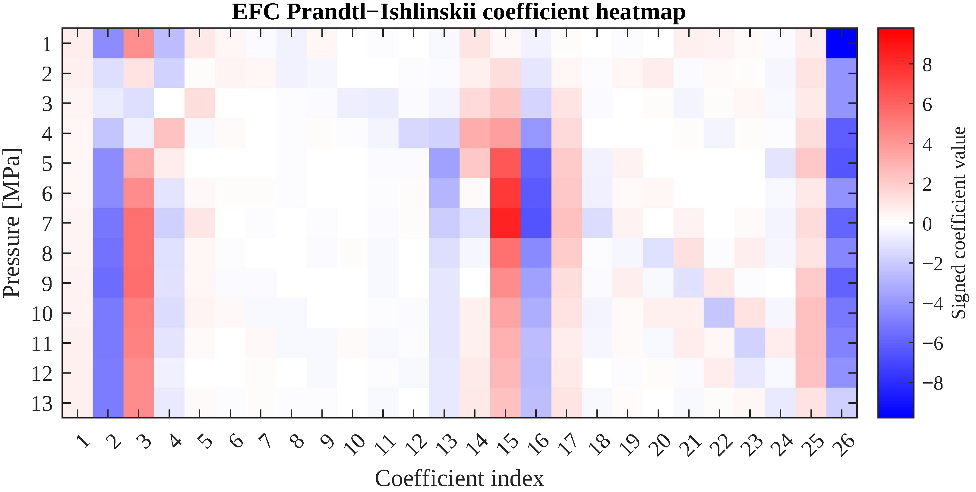
Figure A1 summarizes the pressure-wise coefficient vectors for the two operator-based models. The common threshold vector is not repeated in the figure because it is shared across all pressure levels.
Figure A1. Pressure-wise coefficient maps for the EFC dataset. The upper panel shows the Prandtl–Ishlinskii coefficient vector w, and the lower panel shows the Maxwell-slip coefficient vector w.
Actuators 15 00257 g0a1aActuators 15 00257 g0a1b

Appendix A.1.2. Preisach Representation

Figure A2 depicts the relay-associated Preisach weights on the common lattice G for all pressure levels. This representation follows the standard Preisach-plane view and replaces a much longer printed list of ( α , β , w ) triplets.
Figure A2. Preisach-plane relay-weight maps for the EFC dataset. Each panel corresponds to one pressure level.
Actuators 15 00257 g0a2

Appendix A.1.3. Bouc–Wen Parameters

Table A1 reports the identified Bouc–Wen parameter vector θ = [ A , β , γ , n , b 0 , b 1 , b 2 , k z ] for each pressure level.
Table A1. Identified Bouc–Wen parameters for the EFC dataset.
Pressure [MPa]A β γ n b 0 b 1 b 2 k z
0.008.966360.295194.999881.942010.851412−2.466431.19629−0.133995
0.053.924120.902184.9919110.819681−2.514771.4151−0.279839
0.101.312960.044909−0.5935231.686580.7756252.482894.99982−4.99999
0.151.464210.0370822−0.4881722.046450.6820992.944245−4.77722
0.200.9571310.18291−1.745761.17450.591575−1.640745−1.96542
0.250.8311070.242901−1.976351.000110.565375−1.730914.70215−1.78651
0.309.7527419.6614−3.161063.622480.593938−1.986721.19984−0.199895
0.3519.842115.998351.935160.65179−2.027221.08219−0.190875
0.402013.519351.702420.685264−2.075011.04664−0.175411
0.4519.999814.652651.406810.7228−2.127921.01811−0.175183
0.502016.031551.639290.738296−2.100290.929933−0.177954
0.5519.954715.620451.959240.752924−2.09010.868341−0.167315
0.603.0200619.992951.000070.766832−2.071940.795438−1.32964

Appendix A.2. MFC Dataset

Appendix A.2.1. Prandtl–Ishlinskii and Maxwell-Slip Representations
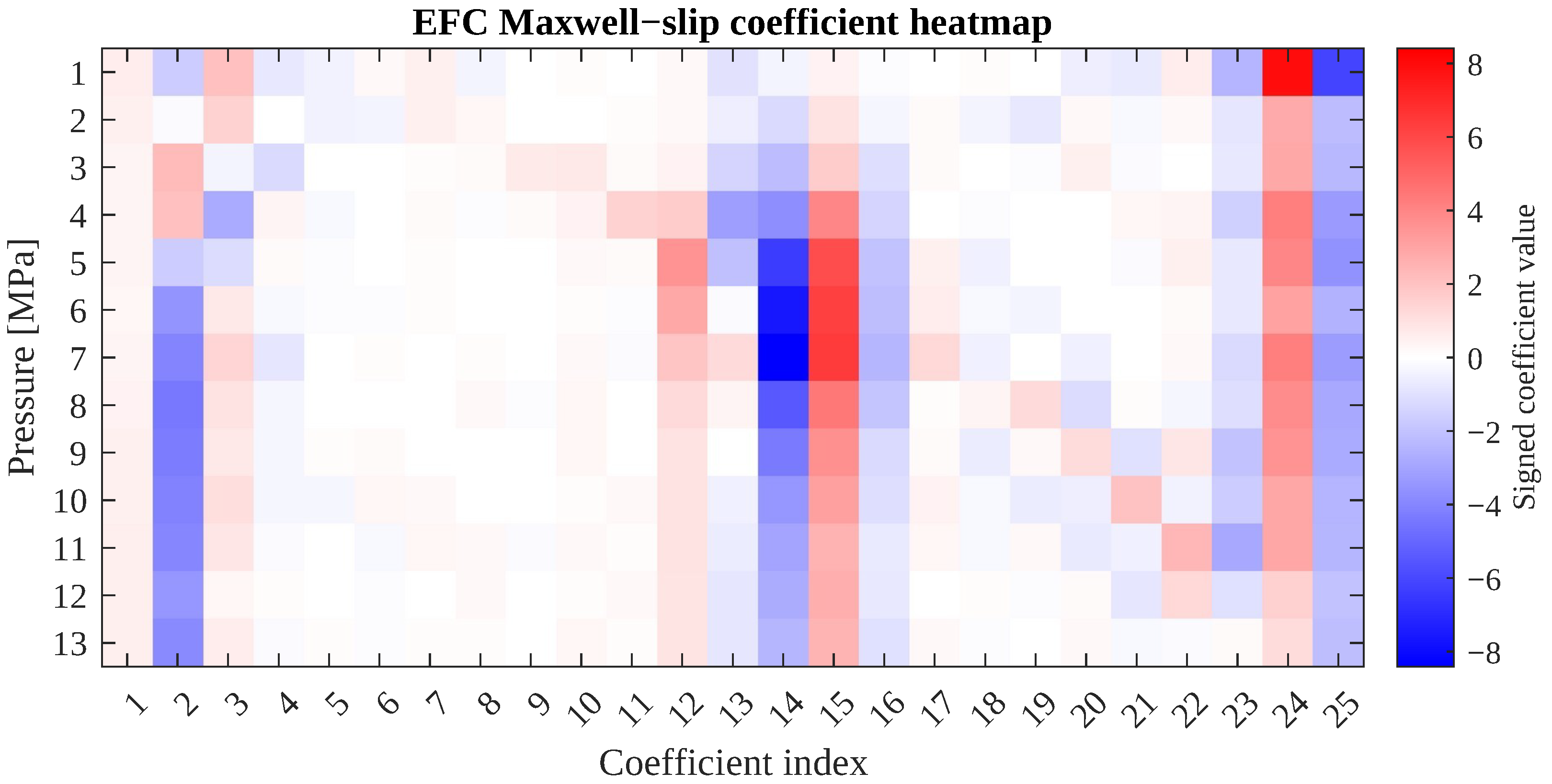
Figure A3 summarizes the pressure-wise coefficient vectors for the two operator-based models. The common threshold vector is not repeated in the figure because it is shared across all pressure levels.
Figure A3. Pressure-wise coefficient maps for the MFC dataset. The upper panel shows the Prandtl–Ishlinskii coefficient vector w, and the lower panel shows the Maxwell-slip coefficient vector w.
Actuators 15 00257 g0a3

Appendix A.2.2. Preisach Representation
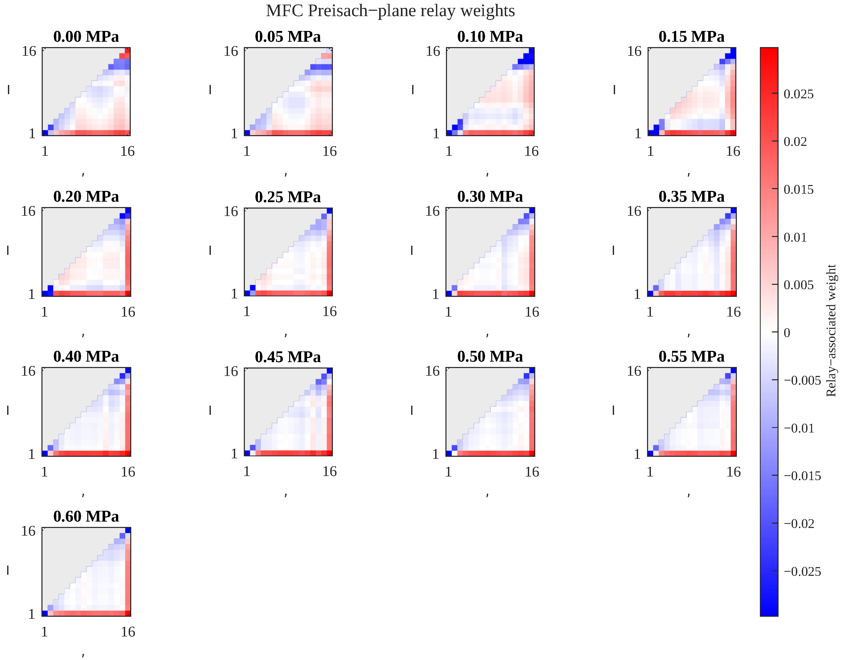
Figure A4 depicts the relay-associated Preisach weights on the common lattice G for all pressure levels. This representation follows the standard Preisach-plane view and replaces a much longer printed list of ( α , β , w ) triplets.
Figure A4. Preisach-plane relay-weight maps for the MFC dataset. Each panel corresponds to one pressure level.
Actuators 15 00257 g0a4

Appendix A.2.3. Bouc–Wen Parameters

Table A2 reports the identified Bouc–Wen parameter vector θ = [ A , β , γ , n , b 0 , b 1 , b 2 , k z ] for each pressure level.
Table A2. Identified Bouc–Wen parameters for the MFC dataset.
Pressure [MPa]A β γ n b 0 b 1 b 2 k z
0.007.166460.2530874.997752.716830.900393−2.600371.21952−0.126326
0.05200.012743752.86120.909773−2.832261.57029−0.0773727
0.101.47970.02873−0.4771141.805510.8168263.226275−4.99969
0.151.0660.0547901−0.8160161.949850.7179971.255065−4.99999
0.200.6394470.18405−2.01631.157310.627058−1.979425−2.48314
0.250.5948670.201875−2.004721.000050.578738−1.750134.76274−2.43202
0.300.5541620.157467−1.800441.000030.589907−1.32884.85895−3.32496
0.3513.707819.99964.420422.240660.667867−2.069831.09667−0.204684
0.4019.99911.0651.7820.706936−2.139531.07721−0.137255
0.4518.423113.069851.352970.742918−2.182291.03767−0.145723
0.5010.780819.91984.997831.561190.769178−2.189690.969008−0.245538
0.5513.244219.99943.79341.979930.781138−2.179820.915686−0.180087
0.602.5914419.950151.001830.753523−2.073070.834604−1.14468

References

  1. Chou, C.P.; Hannaford, B. Measurement and modeling of McKibben pneumatic artificial muscles. IEEE Trans. Robot. Autom. 1996, 21, 90–102. [Google Scholar] [CrossRef] [Scilit]
  2. Tondu, B.; Lopez, P. Modeling and control of McKibben artificial muscle robot actuators. IEEE Control Syst. 2000, 20, 15–38. [Google Scholar] [CrossRef] [Scilit]
  3. Ganguly, S.; Garg, A.; Pasricha, A.; Dwivedy, S. Control of pneumatic artificial muscle system through experimental modelling. Mechatronics 2012, 22, 1135–1147. [Google Scholar] [CrossRef] [Scilit]
  4. Zhang, Y.; Liu, H.; Ma, T.; Hao, L.; Li, Z. A comprehensive dynamic model for pneumatic artificial muscles considering different input frequencies and mechanical loads. Mech. Syst. Signal Process. 2021, 148, 107133. [Google Scholar] [CrossRef] [Scilit]
  5. Kalita, B.; Leonessa, A.; Dwivedy, S.K. A Review on the Development of Pneumatic Artificial Muscle Actuators: Force Model and Application. Actuators 2022, 11, 288. [Google Scholar] [CrossRef] [Scilit]
  6. Tondu, B. Robust and Accurate Closed-Loop Control of McKibben Artificial Muscle Contraction with a Linear Single Integral Action. Actuators 2014, 3, 142–161. [Google Scholar] [CrossRef] [Scilit]
  7. Nguyen, M.K.; Trinh, V.C.; Vo, N.Y.P.; Le, T.D. Restoring Model of a Pneumatic Artificial Muscle with Structure Parameters: Analysis and Identification. Actuators 2024, 13, 355. [Google Scholar] [CrossRef] [Scilit]
  8. Trinh, V.C.; Vo, N.Y.P.; Luu, T.T.; Le, T.D. Dynamic model of air spring based McKibben pneumatic artificial muscle. Commun. Nonlinear Sci. Numer. Simul. 2025, 147, 108829. [Google Scholar] [CrossRef] [Scilit]
  9. Andrikopoulos, G.; Nikolakopoulos, G.; Arvanitakis, I.; Manesis, S. Piecewise Affine Modeling and Constrained Optimal Control for a Pneumatic Artificial Muscle. IEEE Trans. Ind. Electron. 2014, 61, 904–916. [Google Scholar] [CrossRef] [Scilit]
  10. Andrikopoulos, G.; Nikolakopoulos, G.; Arvanitakis, I.; Manesis, S. Switching model predictive control of a pneumatic artificial muscle. Int. J. Control. Autom. Syst. 2013, 11, 1223–1231. [Google Scholar] [CrossRef] [Scilit]
  11. Zhao, L.; Cheng, H.; Zhang, J.; Xia, Y. Adaptive control for a motion mechanism with pneumatic artificial muscles subject to dead-zones. Mech. Syst. Signal Process. 2021, 148, 107155. [Google Scholar] [CrossRef] [Scilit]
  12. Qin, Y.; Xu, Y.; Shen, C.; Han, J. High-Precision Displacement and Force Hybrid Modeling of Pneumatic Artificial Muscle Using 3D PI-NARMAX Model. Actuators 2022, 11, 51. [Google Scholar] [CrossRef] [Scilit]
  13. Saito, N.; Satoh, T.; Saga, N. Double Air Chambers Pneumatic Artificial Muscle and Non-Hysteresis Position Control. Actuators 2024, 13, 282. [Google Scholar] [CrossRef] [Scilit]
  14. Lin, C.J.; Lin, C.R.; Yu, S.K.; Chen, C.T. Hysteresis modeling and tracking control for a dual pneumatic artificial muscle system using Prandtl-Ishlinskii model. Mechatronics 2015, 28, 35–45. [Google Scholar] [CrossRef] [Scilit]
  15. Liu, Y.; Zang, X.; Lin, Z.; Liu, X.; Zhao, J. Modelling Length/Pressure Hysteresis of a Pneumatic Artificial Muscle using a Modified Prandtl-Ishlinskii Model. Stroj. Vestn.-J. Mech. Eng. 2017, 63, 56–64. [Google Scholar] [CrossRef] [Scilit]
  16. Qin, Y.; Zhang, H.; Wang, X.; Han, J. Active Model-Based Hysteresis Compensation and Tracking Control of Pneumatic Artificial Muscle. Sensors 2022, 22, 364. [Google Scholar] [CrossRef] [Scilit]
  17. Xie, S.; Zhong, H.; Zhang, J.; Li, Y.; Xu, S. Modeling, identification, and compensation control of pneumatic muscle hysteresis based on an improved generalized Bouc-Wen model. Measurement 2025, 253, 117512. [Google Scholar] [CrossRef] [Scilit]
  18. Mishra, M.K.; Samantaray, A.K.; Chakraborty, G. Fractional-order Bouc-wen hysteresis model for pneumatically actuated continuum manipulator. Mech. Mach. Theory 2022, 173, 104841. [Google Scholar] [CrossRef] [Scilit]
  19. Soleymani, R.; Khajehsaeid, H. A mechanical model for McKibben pneumatic artificial muscles based on limiting chain extensibility and 3D application of the network alteration theories. Int. J. Solids Struct. 2020, 202, 620–630. [Google Scholar] [CrossRef] [Scilit]
  20. Csikós, S.; Mészáros, A.; Sárosi, J. Pressure-Dependent Hysteresis in a Spring–Rod Compact Pneumatic Artificial Muscle Compared with a Commercial McKibben Actuator. Actuators 2026, 15, 80. [Google Scholar] [CrossRef] [Scilit]
  21. Sárosi, J. Estimated Force-Contraction Curves of Fluidic Muscles by a Five-Parameter Function. In Proceedings of the 7th International Conference for Young Researchers and Ph.D. Students: Education, Research, Innovation (ERIN 2013), Bratislava, Slovakia, 15–17 May 2013; pp. 1–6. [Google Scholar]
  22. Sárosi, J.; Fabulya, Z. Mathematical Analysis of the Function Approximation for the Force Generated by Pneumatic Artificial Muscle. Sci. Bull. Politeh. Univ. Timis. Trans. Mech. 2012, 57, 59–64. [Google Scholar]
  23. Chua, L.O. Memristor-The Missing Circuit Element. IEEE Trans. Circuit Theory 1971, 18, 507–519. [Google Scholar] [CrossRef] [Scilit]
  24. Chua, L.O.; Kang, S.M. Memristive devices and systems. Proc. IEEE 1976, 64, 209–223. [Google Scholar] [CrossRef] [Scilit]
  25. Pershin, Y.V.; Ventra, M.D. Memory effects in complex materials and nanoscale systems. Adv. Phys. 2011, 60, 145–227. [Google Scholar] [CrossRef] [Scilit]
  26. Ventra, M.D.; Pershin, Y.V. On the physical properties of memristive memcapacitive and meminductive systems. Nanotechnology 2013, 24, 255201. [Google Scholar] [CrossRef] [Scilit]
  27. Singh, J.; Raj, B. Comparative analysis of memristor models and memories design. J. Semicond. 2018, 39, 074006. [Google Scholar] [CrossRef] [Scilit]
  28. Vongehr, S. The Missing Memristor has Not been Found. Sci. Rep. 2015, 5, 11657. [Google Scholar] [CrossRef] [Scilit] [PubMed]
  29. Chua, L. Resistance switching memories are memristors. Appl. Phys. A 2011, 102, 765–783. [Google Scholar] [CrossRef] [Scilit]
  30. Paulo, G.; Sun, K.; Di Muccio, G.; Gubbiotti, A.; Morozzo della Rocca, B.; Geng, J.; Maglia, G.; Chinappi, M.; Giacomello, A. Hydrophobically gated memristive nanopores for neuromorphic applications. Nat. Commun. 2023, 14, 8390. [Google Scholar] [CrossRef] [Scilit]
  31. Wei, X.; Wu, Z.; Gao, H.; Cao, S.; Meng, X.; Lan, Y.; Su, H.; Qin, Z.; Liu, H.; Du, W.; et al. Mechano-gated iontronic piezomemristor. Nat. Commun. 2025, 16, 1060. [Google Scholar] [CrossRef] [Scilit] [PubMed]
  32. He, Y.; LV, H.; Zhang, Y.; Si, W.; Sha, J.; Chen, Y.; Ma, J. Mechano-Gated Nanofluidic Piezomemristor: Elastic Nanochannel Bridging Dynamic Pressure Modulation and Neuromorphic Plasticity. ACS Appl. Mater. Interfaces 2025, 17, 50292–50301. [Google Scholar] [CrossRef] [Scilit]
  33. Robin, P.; Kavokine, N.; Bocquet, L. Modeling of emergent memory and voltage spiking in ionic transport through angstrom-scale slits. Science 2021, 373, 687–691. [Google Scholar] [CrossRef] [Scilit]
  34. Xiong, T.; Li, C.; He, X.; Xie, B.; Zong, J.; Jiang, Y.; Ma, W.; Wu, F.; Fei, J.; Yu, P.; et al. Neuromorphic functions with a polyelectrolyte-confined fluidic memristor. Science 2023, 379, 156–161. [Google Scholar] [CrossRef] [Scilit]
  35. Robin, P.; Emmerich, T.; Ismail, A.; Niguès, A.; You, Y.; Nam, G.H.; Keerthi, A.; Siria, A.; Geim, A.K.; Radha, B.; et al. Long-term memory and synapse-like dynamics in two-dimensional nanofluidic channels. Science 2023, 379, 156–161. [Google Scholar] [CrossRef] [Scilit]
  36. Emmerich, T.; Teng, Y.; Ronceray, N.; Lopriore, E.; Chiesa, R.; Chernev, A.; Artemov, V.; Ventra, M.D.; Kis, A.; Radenovic, A. Nanofluidic logic with mechano-ionic memristive switches. Nat. Electron. 2024, 7, 271–278. [Google Scholar] [CrossRef] [Scilit] [PubMed]
  37. Zhou, X.; Zong, Y.; Wang, Y.; Sun, M.; Shi, D.; Wang, W.; Du, G.; Xie, Y. Nanofluidic memristor based on the elastic deformation of nanopores with nanoparticle adsorption. Natl. Sci. Rev. 2024, 11, nwad216. [Google Scholar] [CrossRef] [Scilit] [PubMed]
  38. Wang, D.; Kvetny, M.; Liu, J.; Brown, W.; Li, Y.; Wang, G. Transmembrane Potential across Single Conical Nanopores and Resulting Memristive and Memcapacitive Ion Transport. J. Am. Chem. Soc. 2012, 134, 3651–3654. [Google Scholar] [CrossRef] [Scilit] [PubMed]
  39. Xu, G.; Zhang, M.; Mei, T.; Liu, W.; Wang, L.; Xiao, K. Nanofluidic Ionic Memristors. ACS Nano 2024, 18, 19423–19442. [Google Scholar] [CrossRef] [Scilit]
  40. Shi, D.; Wang, W.; Liang, Y.; Duan, L.; Du, G.; Xie, Y. Ultralow Energy Consumption Angstrom-Fluidic Memristor. Nano Lett. 2023, 23, 11662–11668. [Google Scholar] [CrossRef] [Scilit]
  41. Mayergoyz, I.D. The Classical Preisach Model of Hysteresis. In Mathematical Models of Hysteresis; Springer: New York, NY, USA, 1991; pp. 1–63. [Google Scholar] [CrossRef] [Scilit]
  42. Firestone, F.A. A new analogy between mechanical and electrical systems. J. Acoust. Soc. Am. 1933, 4, 249–267. [Google Scholar] [CrossRef] [Scilit]
  43. Bertuccio, G. On the physical origin of the electro-mechano-acoustical analogy. J. Acoust. Soc. Am. 2022, 151, 2066–2076. [Google Scholar] [CrossRef] [Scilit] [PubMed]
  44. Smith, M.C. Synthesis of mechanical networks: The inerter. IEEE Trans. Autom. Control 2002, 47, 1648–1662. [Google Scholar] [CrossRef] [Scilit]
  45. Chen, M.; Papageorgiou, C.; Scheibe, F.; Wang, F.c.; Smith, M. The missing mechanical circuit element. IEEE Circuits Syst. Mag. 2009, 9, 10–26. [Google Scholar] [CrossRef] [Scilit]
  46. Oster, G.F.; Auslander, D.M. The Memristor: A New Bond Graph Element. J. Dyn. Syst. Meas. Control 1972, 94, 249–252. [Google Scholar] [CrossRef] [Scilit]
  47. Pei, J.S.; Wright, J.P.; Todd, M.D.; Masri, S.F.; Gay-Balmaz, F. Understanding memristors and memcapacitors in engineering mechanics applications. Nonlinear Dyn. 2015, 80, 457–489. [Google Scholar] [CrossRef] [Scilit]
  48. Oster, G. A note on memristors. IEEE Trans. Circuits Syst. 1974, 2, 152. [Google Scholar] [CrossRef] [Scilit]
Figure 1. Experimental measurement setup used for the compact-PAM dataset.
Actuators 15 00257 g001
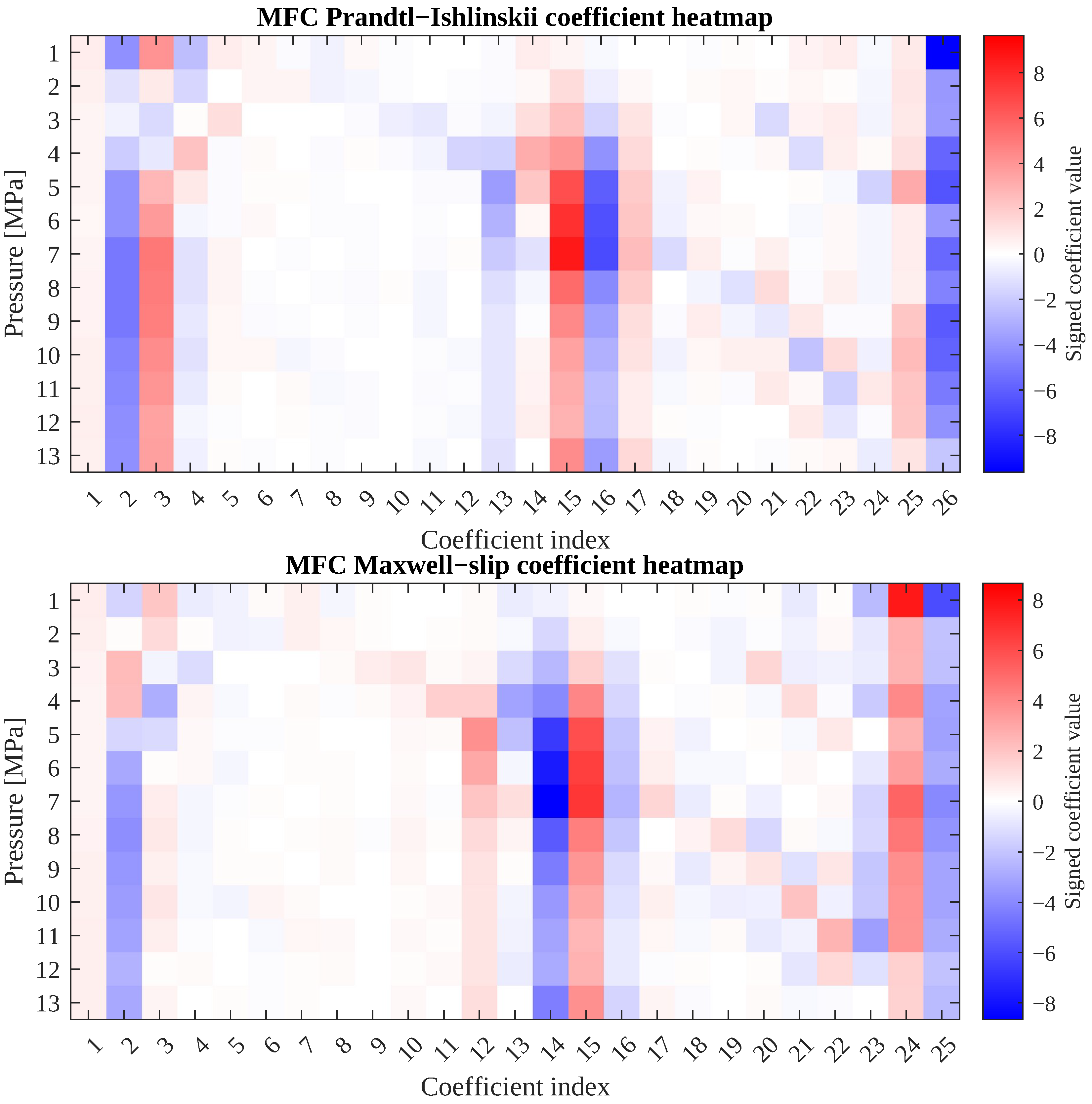
Figure 2. Schematic representation of the experimental measurement setup.
Actuators 15 00257 g002
Figure 3. Tiled fit comparison between the measured MFC data and the identified branch surfaces.
Actuators 15 00257 g003
Figure 4. Tiled fit comparison between the measured EFC data and the identified branch surfaces.
Actuators 15 00257 g004
Figure 5. Residuals and error maps for the MFC surfaces.
Actuators 15 00257 g005
Figure 6. Residuals and error maps for the EFC surfaces.
Actuators 15 00257 g006
Figure 7. Measured force–contraction curves at p = 0.00 , 0.10 , 0.20 , 0.30 , 0.40 , 0.50 , and 0.60 MPa .
Actuators 15 00257 g007
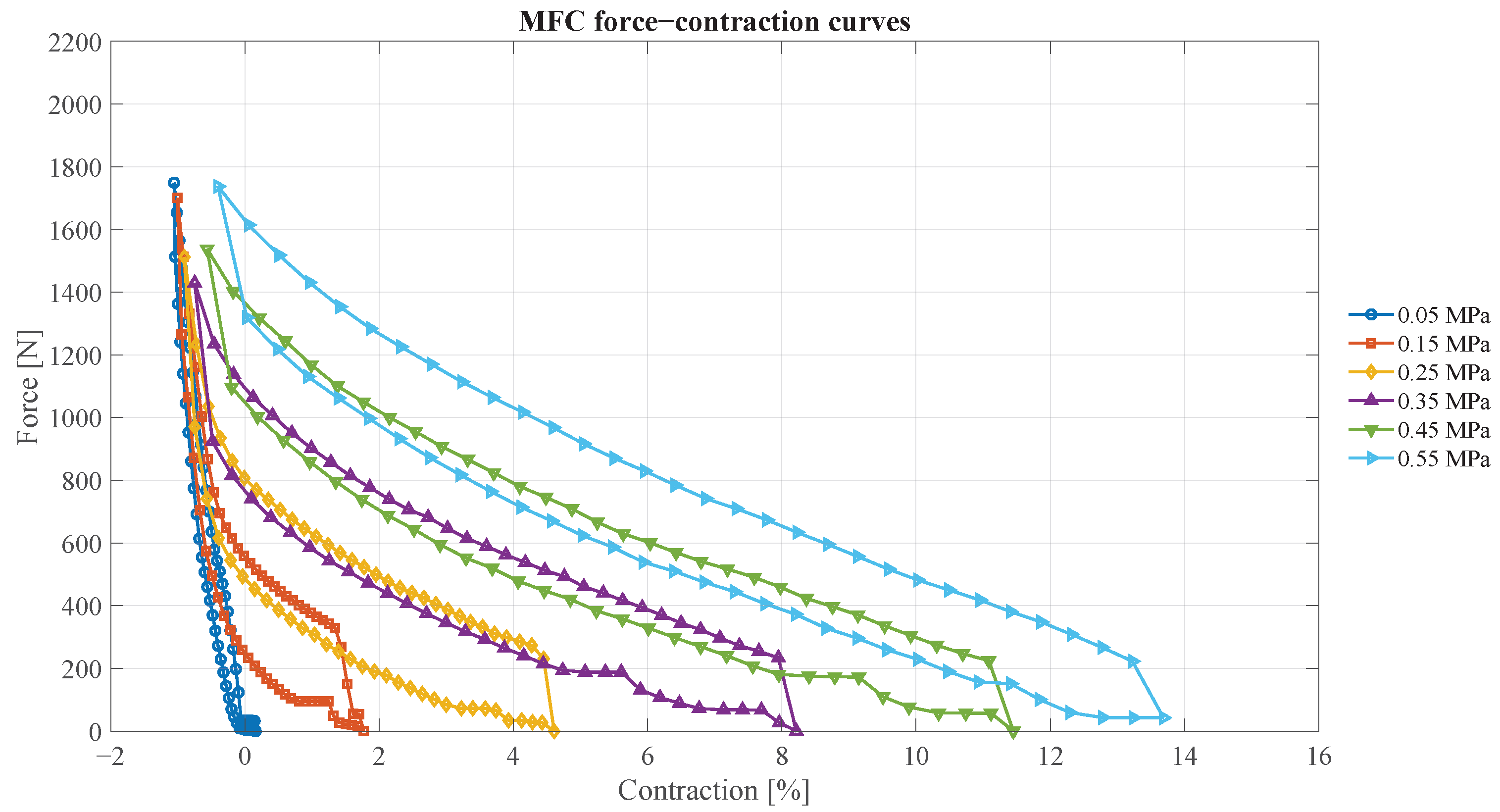
Figure 8. Measured force–contraction curves at p = 0.05 , 0.15 , 0.25 , 0.35 , 0.45 , and 0.55 MPa .
Actuators 15 00257 g008
Figure 9. Excitation force–contraction curves at p = 0.00 , 0.10 , 0.20 , 0.30 , 0.40 , 0.50 , and 0.60 MPa .
Actuators 15 00257 g009
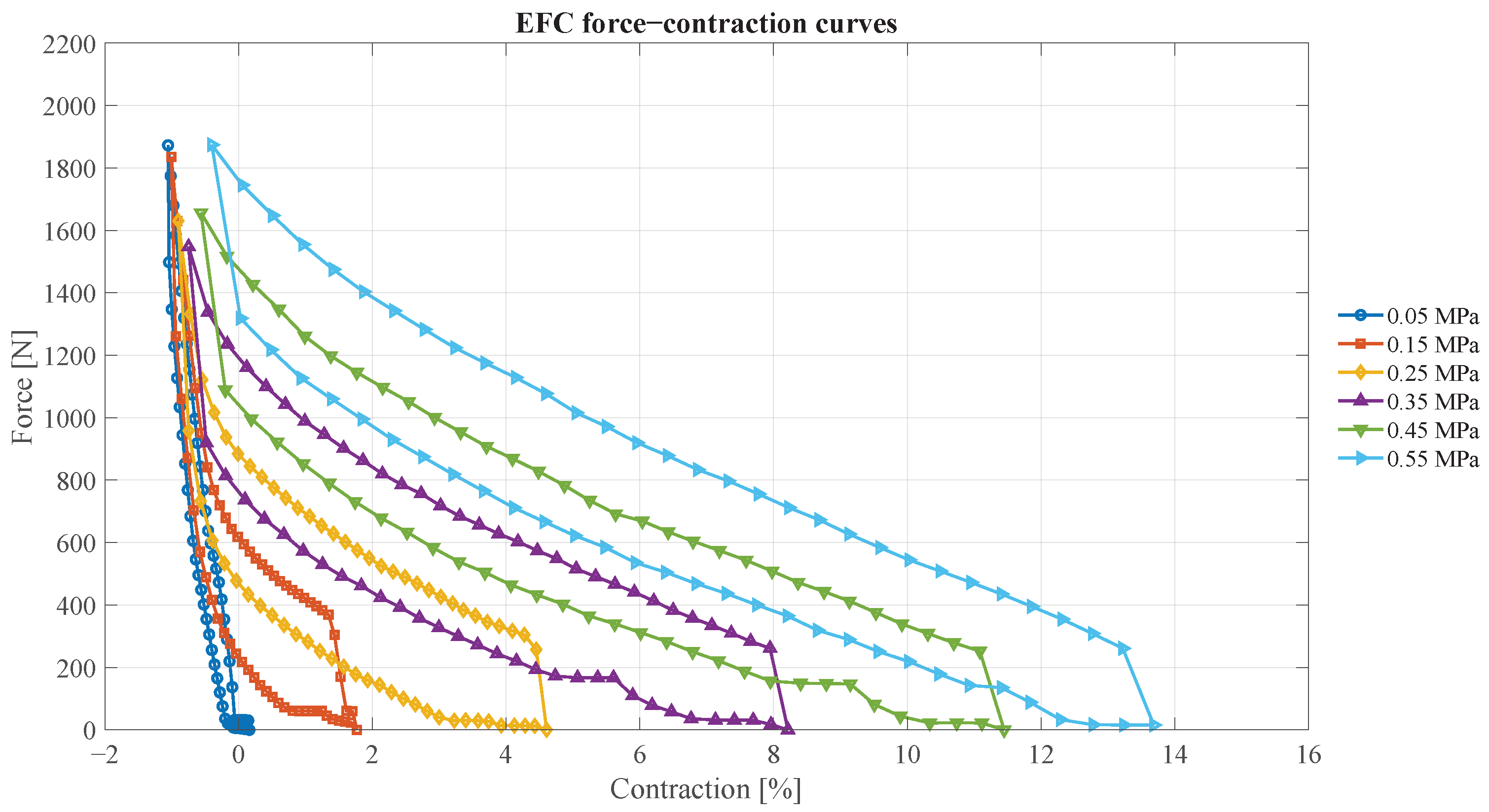
Figure 10. Excitation force–contraction curves at p = 0.05 , 0.15 , 0.25 , 0.35 , 0.45 , and 0.55 MPa .
Actuators 15 00257 g010
Figure 11. PI fit overlays for MFC values grouped by pressure.
Actuators 15 00257 g011
Figure 12. PI fit residuals for MFC values.
Actuators 15 00257 g012
Figure 13. PI fit overlays for EFC values grouped by pressure.
Actuators 15 00257 g013
Figure 14. PI fit residuals for EFC values.
Actuators 15 00257 g014
Figure 15. BoucWen fit overlays for MFC values grouped by pressure.
Actuators 15 00257 g015
Figure 16. BoucWen fit residuals for MFC values.
Actuators 15 00257 g016
Figure 17. BoucWen fit overlays for EFC values grouped by pressure.
Actuators 15 00257 g017
Figure 18. BoucWen fit residuals for EFC values.
Actuators 15 00257 g018
Figure 19. Preisach fit overlays for MFC values grouped by pressure.
Actuators 15 00257 g019
Figure 20. Preisach fit residuals for MFC values.
Actuators 15 00257 g020
Figure 21. Preisach fit overlays for EFC values grouped by pressure.
Actuators 15 00257 g021
Figure 22. Preisach fit residuals for EFC values.
Actuators 15 00257 g022
Figure 23. Maxwell-slip fit overlays for MFC values grouped by pressure.
Actuators 15 00257 g023
Figure 24. Maxwell-slip fit residuals for MFC values.
Actuators 15 00257 g024
Figure 25. Maxwell-slip fit overlays for EFC values grouped by pressure.
Actuators 15 00257 g025
Figure 26. Maxwell-slip fit residuals for EFC values.
Actuators 15 00257 g026
Figure 27. Memristive fit overlays for MFC values grouped by pressure.
Actuators 15 00257 g027
Figure 28. Memristive fit residuals for MFC values.
Actuators 15 00257 g028
Figure 29. Memristive fit overlays for EFC values grouped by pressure.
Actuators 15 00257 g029
Figure 30. Memristive fit residuals for EFC values.
Actuators 15 00257 g030
Figure 31. Sensitivity to alpha.
Actuators 15 00257 g031
Table 1. Electrical-mechanical correspondences used to interpret the compact-PAM hysteresis model. The impedance analogy column is the one adopted in this paper.
Electrical RelationAdopted Impedance AnalogyAlternative Mobility Analogy
U effort, I flow F effort, v flow v effort, F flow
q = I d t , φ = U d t s = v d t , p m = F d t s = v d t , p m = F d t
P = U I P = F v P = F v
U = R I or I = G U F = b v , so R b F = b v , so G b and equivalently R 1 / b
W R = U I d t = R I 2 d t W b = F v d t = b v 2 d t W b = F v d t = b v 2 d t
U L = L d I / d t F = m d v / d t , so L m v = c d F / d t with c = 1 / k , so L c
E L = 1 2 L I 2 = φ 2 2 L E kin = 1 2 m v 2 = p m 2 2 m E el = 1 2 c F 2 = s 2 2 c
I C = C d U / d t v = c d F / d t with c = 1 / k , so C c F = m d v / d t , so C m
E C = 1 2 C U 2 = q 2 2 C E el = 1 2 c F 2 = s 2 2 c E kin = 1 2 m v 2 = p m 2 2 m
U M = R ( x , I , t ) I , x ˙ = f ( x , I , t ) Generalized state-dependent one-port description for the CPAM
Notation used in Table 1: U and I denote electrical effort and flow variables, q electric charge, φ magnetic flux linkage, and P instantaneous power. The parameters R, G, L, and C denote resistance, conductance, inductance, and capacitance. On the mechanical side, F and v are force and velocity, s is displacement, and p m = F d t is the time integral of force. The parameters b, m, k, and c = 1 / k denote viscous damping, mass, spring stiffness, and compliance. The displacement symbol s in the table should not be confused with the branch indicator s n used later in the state-update law.
Table 2. Identified five-parameter Sárosi–Fabulya coefficients at 4 N / s together with fit-quality metrics.
Surface a 1 (95% CI) a 2 (95% CI) a 3 (95% CI) a 4 (95% CI) a 5 (95% CI) R 2 Adjusted R 2 RMSE
EFC unload283.5532 [281.6804; 285.4260]−1.7535 [−1.7601; −1.7470]−152.8966 [−153.4096; −152.3837]2719.0 [2713.3; 2724.7]−444.4829 [−446.6841; −442.2817]0.99870.998715.5383
EFC load299.2673 [296.7116; 301.8231]−1.7530 [−1.7617; −1.7444]−189.3924 [−190.0839; −188.7009]3175.5 [3167.8; 3183.2]−195.3742 [−198.3438; −192.4046]0.99790.997920.9446
MFC unload253.8404 [250.9353; 256.7456]−1.8403 [−1.8517; −1.8288]−149.5208 [−150.3456; −148.6961]2591.3 [2582.0; 2600.5]−383.4218 [−386.9346; −379.9091]0.99630.996325.1240
MFC load277.6454 [275.4956; 279.7953]−1.7597 [−1.7675; −1.7518]−175.9270 [−176.5101; −175.3438]2910.6 [2904.1; 2917.2]−188.3115 [−190.8145; −185.8085]0.99820.998217.6720
Table 3. Normalized hysteresis index as a function of pressure for the EFC and MFC cases. The index is reported in percent.
Pressure [MPa]EFC NHI [%]MFC NHI [%]
0.0014.71911.770
0.0515.15512.471
0.1016.30913.716
0.1518.04715.335
0.2020.23317.163
0.2521.07418.070
0.3021.48118.370
0.3523.29719.507
0.4022.50418.756
0.4520.65816.658
0.5020.13616.341
0.5518.74614.964
0.6018.03713.588
Table 4. Overall model comparison for the EFC and MFC cases. Lower RMSE and maximum absolute error (MaxAE) indicate better performance, whereas higher R 2 indicates better goodness of fit. The best value for each metric within each case is shown in bold.
EFCMFC
ModelRMSE [N]MaxAE [N] R 2 RMSE [N]MaxAE [N] R 2
Bouc–Wen64.278543.600.9812355.541488.350.98360
Maxwell-slip107.510915.270.9475099.456817.450.94740
Memristive110.160587.810.94488100.880541.530.94589
PI106.020876.490.9489598.066783.770.94886
Preisach51.958382.190.9877443.364360.760.99000
Disclaimer/Publisher’s Note: The statements, opinions and data contained in all publications are solely those of the individual author(s) and contributor(s) and not of MDPI and/or the editor(s). MDPI and/or the editor(s) disclaim responsibility for any injury to people or property resulting from any ideas, methods, instructions or products referred to in the content.