Numerical Investigation of Plasma-Based Active Flow Control on Heaving-Pitching NACA0015 Airfoil via Large Eddy Simulation

Abstract

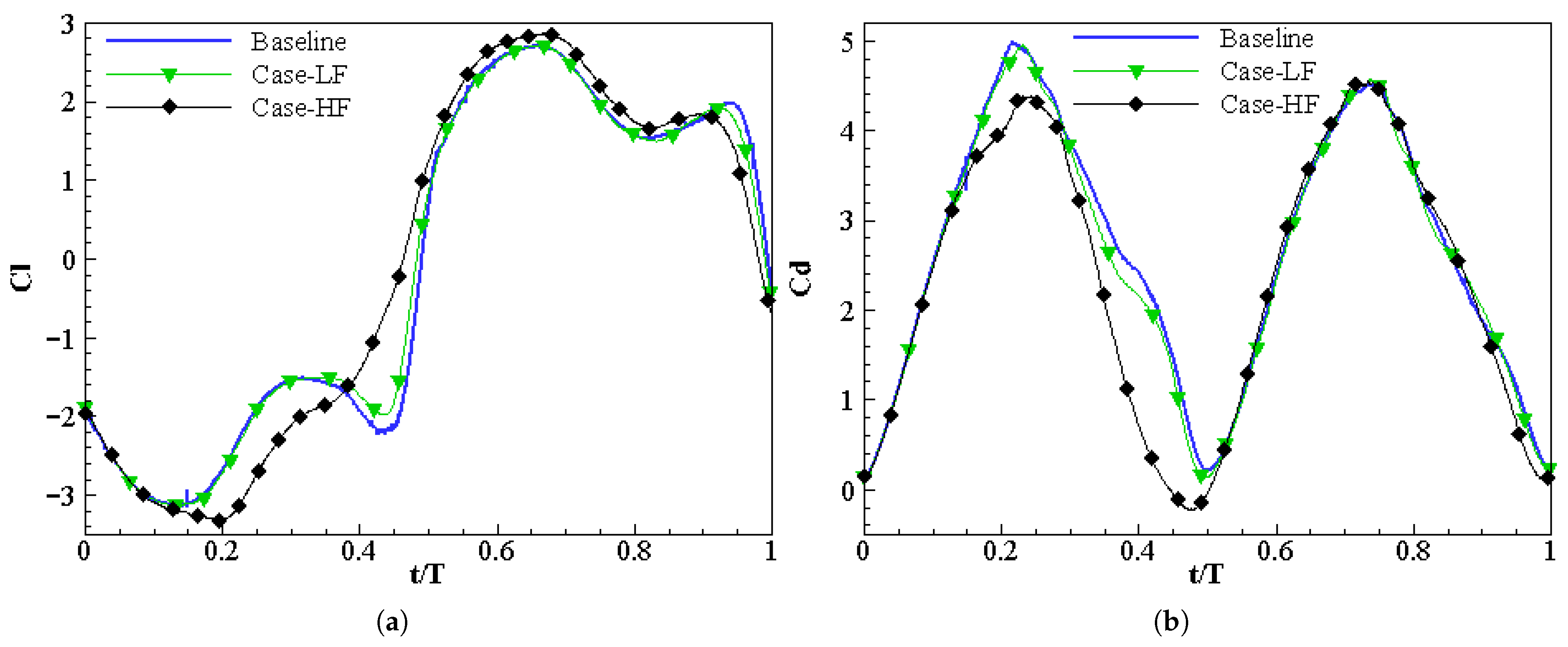
This study implements Active Flow Control (AFC) in the form of a dielectric barrier discharge (DBD) plasma actuator to enhance aerodynamic performance during heave–pitch motions on a three-dimensional NACA 0015 airfoil at a Reynolds number of $Re=5\times {10}^5$ using the Large Eddy Simulation (LES) turbulence method. The simulation at a reduced frequency of 0.14 incorporates two-degrees-of-freedom wing motion, allowing for simultaneous pitching and heaving motions with amplitudes of ${75}^{\circ }$ and a chord length ($1c$), respectively. We evaluate the impact of localized momentum injection via a phenomenological plasma actuator model across two force intensities. A low-force configuration (Case-LF) provides marginal control, whereas a high-force configuration (Case-HF) provides greater control than the baseline without plasma. After applying DBD plasma to the airfoil, flow-field analysis revealed that the plasma treatment significantly improved the lift coefficient. It showed that the lower plasma cases achieved a 1.46% improvement only on the $C{l}_{rms}$, a 14.57% reduction in the averaged $Cd$, and a 19.11% enhancement on the $C{l}_{rms}$-to-$C{d}_{avg}$ ratio. Furthermore, the cases with higher plasma forces resulted in significant improvements when compared to the Baseline and Case-LF; it showed a 11.65% improvement in $C{l}_{rms}$, 19.87% in $C{d}_{avg}$, and 39.8% in $C{l}_{rms}$-to-$C{d}_{avg}$ ratio when compared to the baseline. These results validate the effectiveness of plasma actuators in enhancing wing aerodynamic performance during such complex motions.

1. Introduction

Flapping wings in aerodynamic applications are based on the principles of birds and insects. Consequently, studies inspired by this have shown that the flapping wing motion is suitable for Micro Aerial Vehicles (MAVs), bio-inspired robotics, and advanced aerospace technologies [1], which led to an understanding of performance optimization and the interaction between the aerodynamics and the kinematic motions of the wing. A wide range of experimental and numerical research has also been conducted to achieve bionic mimicry flight, including pitching, heaving, and rolling motions. Advancements in CFD and experimental techniques for detailed investigations of heave–pitch motions are essential to improve aerodynamic performance, as explained in in the work of Mo et al. [2]. The first study on dynamic heave–pitch motion was conducted by Ham and Garelick [3] for the design of helicopter blades. The heave motion involves vertical oscillation, while the pitch motion refers to angular rotation around the wing’s axis, producing unsteady aerodynamic forces [4]. Kinsey and Dumas [5] performed 2D URANS at a Reynolds number of 500,000 and obtained an energy extraction efficiency of 43%, a center of rotation at $c/3$, a ${90}^{\circ }$ phase angle, a heaving amplitude of 1c, and a pitching amplitude of ${75}^{\circ }$. Similarly, He et al. [6] also performed a simulation of a 2D hydrofoil under comparable conditions using OpenFOAM, achieving an efficiency of 39.68% at a reduced frequency ($f^{*}$) of 0.14 and a pitch amplitude of ${80}^{\circ }$.

This study extends the 2D heave–pitch motion analysis by Mo et al. [2] to a 3D airfoil shape and examines the heave–pitch motion based on the same fluid flow parameters, with flow control by AFC. A more realistic motion of an airfoil can be addressed in this study, rather than a simple motion like 2D pure pitching. It is evident that as the motions become more complex, the flow around the airfoil requires more advanced treatment for enhanced aerodynamic performance. Various studies were conducted to delay flow separation, control dynamic stall, and improve aerodynamic performance by utilizing different passive and active flow control methods, as discussed in detail by Tayebi and Torabi [7]. Among these, AFC methods, such as plasma actuation, show promise for mitigating issues and enhancing aerodynamic performance across different applications [8]. In addition, Sato et al. [9] have shown that plasma actuators can be effective in pure pitching cases. They conducted experiments on a NACA 0015 airfoil with DBD plasma actuators to investigate dynamic stall control for sinusoidal pitching motions. Their results revealed a significant decrease in drag hysteresis and substantial improvements in aerodynamic performance. Omidi [10] discussed how plasma actuators delayed dynamic stall in pitching airfoils at low Reynolds numbers and reported that segmented plasma actuators outperform linear plasma actuators. Other research by Kong et al. [11], Woo and Glezer [12], Visbal [13] and others also shows how DBD plasma actuators effectively delay dynamic stall and enhance performance.

In recent years, the production and usage of aerospace engineering devices have increased, mainly with flapping wings. Inspired by the flapping mechanisms in birds and insects, however, the motions are exposed to dynamic stalls and early flow separations during the oscillation [14]. Helicopter rotors, drones, and surveillance vehicles mostly face the challenge. In light of various research studies on dynamic stalls that challenge the achievement of efficient flight without controlling stalls, the issue escalates when the wing’s angle of attack (AOA) is increased. Smart controlling methods are needed to reduce the effects of dynamic stalls on aerodynamic performance. AFC is one of the flow-controlling types, and DBD plasma actuators are widely used to control and improve the airfoil’s aerodynamic performance. Post and Corke [15] are among the first to apply this method and showed that plasma actuators were effective in dynamic stall control on a NACA 0012 airfoil at high angles of attack, demonstrating a significant delay in the onset of stall. Corke [16] also employed plasma actuation on a sinusoidal inclined airfoil and found an improvement in aerodynamic performance by increasing the lift and decreasing the drag coefficients. Plasma actuators generate body forces with ionized gases in the presence of electric fields, as seen in Figure 1. Their ability to control the behavior of the boundary layer has allowed them to minimize flow separation and successfully delay stalling.

However, previous plasma applications over an airfoil focused on pure pitching motions; the implementation of plasma actuators in combined heave–pitch motions has been minimal due to their complexity and the integration of plasma in the dynamic motion of the airfoils. The experimental complexity and computational cost are also another challenge for researchers. To address these gaps, the current study seeks to apply and evaluate an alternative current DBD (AC-DBD) plasma actuator to a NACA 0015 airfoil in dynamic heave–pitch motions. This work employs the LES turbulence model to capture unsteady flow phenomena, investigating how plasma actuators influence lift enhancement, flow separation control, and dynamic stall mitigation during heave–pitch motions. The results demonstrate the ability of AFC to control the dynamic motions of an airfoil.

2. Numerical Methodology

This study examines the flapping wing motion of a NACA 0015 airfoil. This symmetric airfoil is well-suited to studying these dynamic motions, as its design simplifies the analysis by removing the complexities associated with cambered airfoils. The combined heave–pitch motions were analyzed through computational simulation. Previous research by Lee and Gerontakos [17] has shown that airfoils generate different flow field variations at various AOA, and dynamic stall occurs when the AOA reaches a critical value. AFC in the form of DBD plasma actuators is therefore required to optimize the aerodynamic performance of the airfoil. This study utilizes the AFC technique to control dynamic stall in the heave–pitch motion of an airfoil, employing the open-source OpenFOAM (v4) software. This section introduces the governing equations, DBD plasma formation, solvers in the software, and computational environments used in this study.

2.1. Governing Equations

The Navier–Stokes equation is the governing equation in fluid motion, primarily used to describe the dynamics of viscous fluids [18]. It encompasses the conservation of mass and momentum, as expressed in Equations (1) and (2), respectively. This study uses the conservation of mass and momentum, and these equations are solved using the Finite Volume Method (FVM) with the following equations:

Continuity equation:

$${\displaystyle \frac{\mathsf{\partial }{u}_i}{\mathsf{\partial }{x}_i}}=0i=1\sim 3$$

(1)

Momentum equation:

$${\displaystyle \frac{\mathsf{\partial }{u}_i}{\mathsf{\partial }t}}+{\displaystyle \frac{\mathsf{\partial }\left(u_i{u}_j\right)}{\mathsf{\partial }{x}_j}}=-{\displaystyle \frac{1}{\rho }}{\displaystyle \frac{\mathsf{\partial }p}{\mathsf{\partial }{x}_i}}+\nu {\displaystyle \frac{{\mathsf{\partial }}^2{u}_i}{\mathsf{\partial }{x}_j\mathsf{\partial }{x}_j}}+Fi,j=1\sim 3$$

(2)

where $u_i$ and $u_j$ are components of velocity in x, y, and z directions, $\rho$ is density, p is pressure, $\nu$ is kinematic viscosity, and F is plasma-induced body force.

2.2. Large Eddy Simulation Turbulence Model

LES is an advanced turbulence modeling method that resolves large-scale, energy-containing turbulent eddies and simulates only the small, subgrid-scale motions, offering a balance between efficiency and accuracy for simulating unsteady, three-dimensional turbulent flows [19,20]. This makes LES an ideal model for capturing finer flow-field details and resolving complex fluid dynamics at high Reynolds numbers. In the LES model, numerical methods apply a low-pass filter to the velocity field as shown in Equation (3), separating flow vortices into large and small eddies. LES directly resolves large-scale turbulence eddies, while a subgrid-scale (SGS) model approximates smaller eddies. The low-pass filter excludes vortices with length scales smaller than $\Delta ={\left(\Delta x\Delta y\Delta z\right)}^{1/3}$, while cells within the remaining domain are solved using the Navier–Stokes equations [21], as shown in Equation (4).

The filtered velocity field is defined as follows:

$$\overline{u}\left(x\right)={\int }_{\Delta }G(x-x^{\prime })u^{\prime }\left(x\right)d{x}^{\prime }$$

(3)

The filtered incompressible momentum equation is the governing equation for large-scale flow, which includes a subgrid-scale stress tensor (${\tau }_{ij}$) for the effects of the unresolved scales of turbulence on the flow, as follows:

$${\displaystyle \frac{\mathsf{\partial }{\overline{u}}_i}{\mathsf{\partial }t}}+{\displaystyle \frac{\mathsf{\partial }\left({\overline{u}}_i{\overline{u}}_j\right)}{\mathsf{\partial }{x}_j}}=-{\displaystyle \frac{1}{\rho }}{\displaystyle \frac{\mathsf{\partial }\overline{p}}{\mathsf{\partial }{x}_i}}+\nu {\displaystyle \frac{{\mathsf{\partial }}^2{\overline{u}}_i}{\mathsf{\partial }{x}_j\mathsf{\partial }{x}_j}}-{\displaystyle \frac{\mathsf{\partial }{\tau }_{ij}}{\mathsf{\partial }{x}_j}}+\overline{F}$$

(4)

The equation $\overline{u_i{u}_j}$ in Equation (5), due to its complexity, requires an unfiltered velocity field and can be calculated using an approximate model, expressed as follows:

$${\tau }_{ij}=\overline{u_i{u}_j}-\overline{u_i}\overline{u_j}$$

(5)

In this context, the stress tensor ${\tau }_{ij}$ within the SGS model represents small-scale eddies not resolved by the LES model’s filtering process. This tensor accounts for the difference between actual momentum transfer and the filtered quantities as discussed by Justin and Jonathan [22]. The LES model in this study employs the Smagorinsky model for the SGS representation, for which ${\tau }_{ij}$ can therefore be expressed as

$${\tau }_{ij}-{\displaystyle \frac{1}{3}}{\tau }_{kk}{\delta }_{ij}=-2{\mu }_t\langle S_{ij}\rangle$$

(6)

where ${\delta }_{ij}$ denotes the Kronecker Delta, defining the relationship among various components, $\langle S_{ij}\rangle$ represents the strain rate tensor, as shown in Equation (6), and ${\mu }_t$ in Equation (8) is the eddy viscosity, expressed as

$${\overline{S}}_{ij}={\displaystyle \frac{1}{2}}\left({\displaystyle \frac{\mathsf{\partial }{\overline{u}}_i}{\mathsf{\partial }{x}_j}}+{\displaystyle \frac{\mathsf{\partial }{\overline{u}}_j}{\mathsf{\partial }{x}_i}}\right)$$

(7)

$${\mu }_t=C_s^2\rho {\Delta }^2{\left(\langle S_{ij}\rangle \langle S_{ij}\rangle \right)}^{1/2}$$

(8)

where $C_s$ represents the dimensionless model parameter called the Smagorinsky coefficient, generally between 0.1 and 0.2. In this study, OpenFOAM is used for simulations and $C_s$ can be calculated using Equation (9):

$$C_s=\sqrt{C_k(C_k/C_e}{)}^{1/2}$$

(9)

where $C_k$ in Equation (9) represents the Kolmogorov constant, which is assigned a value of 0.094, while $C_e$ stands for the Smagorinsky constant, set to 1.048. As a result, the value of $C_e$ is calculated to be 0.1678 [23].

2.3. Dynamic Mesh Formulation

A dynamic mesh is employed in OpenFOAM and primarily used to configure the dynamic behavior of objects. Through settings such as sixDoFRigidBodyMotion and solidBodyMotion, etc., the motion of objects within the domain can be specified and constrained [24]. The study uses the sixDoFRigidBodyMotion setting in the dynamicMeshDict, employing the Arbitrary Lagrangian–Eulerian (ALE) method for dynamic mesh processing. Lagrangian methods are commonly used in solid deformation to follow object motion. In contrast, the Eulerian approach fixes the mesh, allowing the fluid to move relative to it, which is ideal for fluid simulations. ALE combines these approaches, permitting the mesh to move either partially as the object moves or entirely with the object as it deforms. This reduces the need to generate new meshes by calculating the rigid body’s position at each time step. As a result, a mesh is deformed and calculated, allowing the object to have degrees of freedom in the flow [25]. This study defines the heave and pitch motions by $\omega$, frequency, heave amplitude, and pitch angle parameters. The pimpleFoam solver combines the PISO and SIMPLE methods, making it suitable for simulating unsteady states in incompressible transient turbulence. The main distinction between pimpleFoam and pimpleDyMFoam lies in “DyM,” which stands for dynamic mesh [24]. As suggested by the name, pimpleDyMFoam supports dynamic meshes, allowing for the inclusion of object motion in fluid simulations while accounting for its effects on the fluid. In our study, the “pimpleDyMFoam” used for the Baseline case, the custom plasma solver “lfpimpleDyMFoam” for the lower force-based plasma actuation case, and “hfpimpleDyMFoam” for the higher force of the plasma actuation case, and accuracy is validated based on the experimental model of Singh et al. [26], and Mukherjee et al. [27].

To resolve the high-fidelity LES framework to allow for it to accurately capture the fragmented shear layers at the $Re=5\times {10}^5$ regime, a constant time step size $\Delta t=5\times {10}^{-4}$ s is utilized for the temporal discretization. This is to ensure that the maximum Courant number is always less than one (CFL < 1) throughout the $T=2.69$ s cycle, resulting in 5385 time steps per cycle to resolve the vortex regularization and pressure fluctuations. This temporal discretization was maintained throughout all cases, including the grid study, validation, and all flow control cases.

3. Computational Setup

3.1. Motion Kinematics

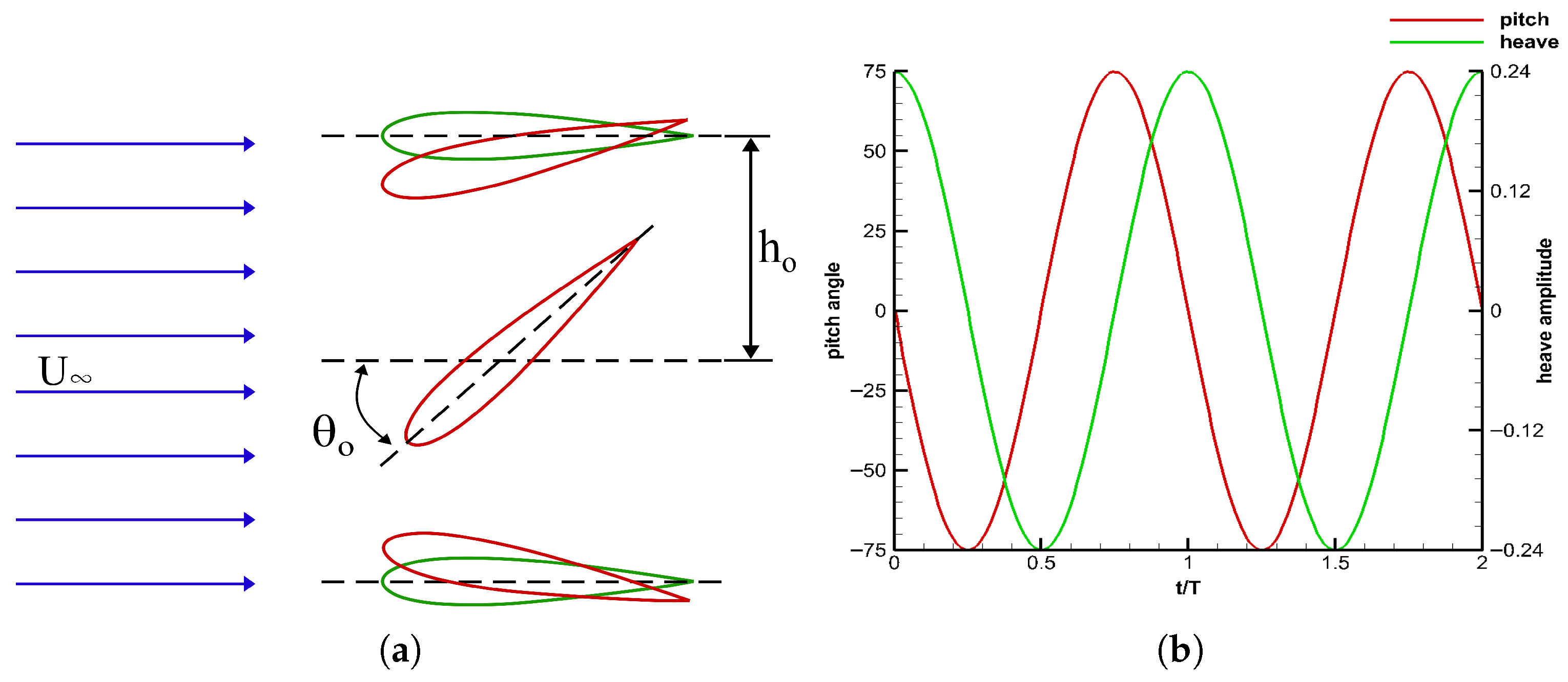
The two degrees of freedom (2-DOF) airfoil motion is expressed by heave and pitch motion equations, as shown in Equation (10), and the heave motion is expressed by Equation (11) [28]. These motions can be represented by distinct sinusoidal waveforms, as illustrated in Figure 1.

The pitch motion is defined as

$$\theta \left(t\right)={\theta }_{0}sin\left(\omega t\right)$$

(10)

The heave motion is defined as

$$h\left(t\right)=h_{0}sin(\omega t+{\phi }_0)$$

(11)

The pitch angle shown as $\theta \left(t\right)$ begins at $0^{\circ }$, shifts to $-{75}^{\circ }$, and then transitions to ${75}^{\circ }$, oscillating cyclically in this range. The pitch amplitude is set to be ${75}^{\circ }$ and shown as ${\theta }_0$, as seen in Figure 1. In heave motion, the heave value $h\left(t\right)$ varies with time, beginning at the maximum value of 0.24 m and initially moving downward, oscillating periodically between 0.24 m and −0.24 m. Heave amplitude is shown as $h_0$, and set to be $h_0$ = 1c = 0.24 m, as in Figure 2. The phase angle ${\phi }_0$ is set to ${90}^{\circ }$ between the two motions.

When expressing the wing’s unsteady motion by the non-dimensionalization of unsteady motion, it is controlled by the chord-based Reynolds number $Re$ and the reduced frequency $f^{*}$. The equations for these are expressed below in Equations (12) and (13), respectively:

$$Re={\displaystyle \frac{U_{\infty }c}{\nu }}$$

(12)

$$f^{*}={\displaystyle \frac{\omega b}{U_{\infty }}}$$

(13)

where $U_{\infty }=2$ m/s is the freestream velocity and $b=c/2=0.12$ m is the half-chord. To achieve the target $Re$, the kinematic viscosity was set to $\nu =9.6\times {10}^{-7}$ m²/s, and the angular velocity is $\omega =2.33$ rad/s, resulting in a full oscillation period of $T=2.69$ s.

3.2. Computational Domain and Mesh Generation

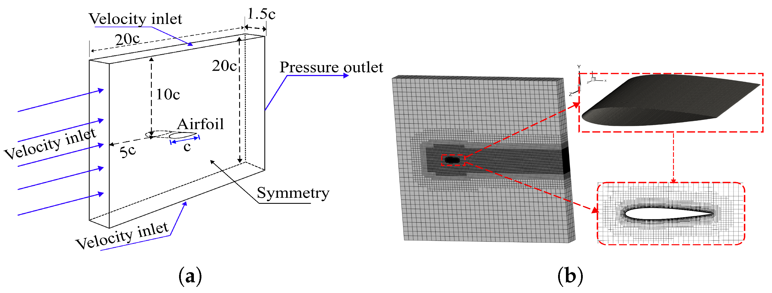
The 3D NACA 0015 airfoil includes a chord length of 0.24 m and a span of 0.375 m. The computational domain extends $20c\times 20c\times 1.5c$ in the streamwise (X-axis) direction, lateral (Y-axis) direction, and spanwise (Z-axis) direction, respectively. The airfoil is placed $5c$ at the inlet and $10c$ at the top and bottom, respectively. To enable detailed observation of downstream flow behavior, the airfoil is located near the front center of the domain. The layout of the computational domain is shown in Figure 2. The blockMesh and snappyHexMesh functions in OpenFOAM were used for grid generation, creating a mesh with 2,168,949 cells, as shown in Figure 2 (the grid independent test is discussed in detail in Section 3.3). As seen in Figure 2b, a crossed dual-refinement approach has been implemented to capture the high velocity gradients induced by plasma body forces. Within the first 1% of the chord (0.01c), the surface is discretized by 50 cells in the chordwise direction, where the plasma is implemented, thereby accurately capturing the resulting velocity gradients and suction peaks without numerical smearing. Then, the simulations for all three cases (Baseline, Case-LF, and Case-HF), each with approximately 2.17 million cells, were run on 64 cores, resulting in a total simulation time of about 1.8 days per cycle.

3.3. Grid-Independent Test

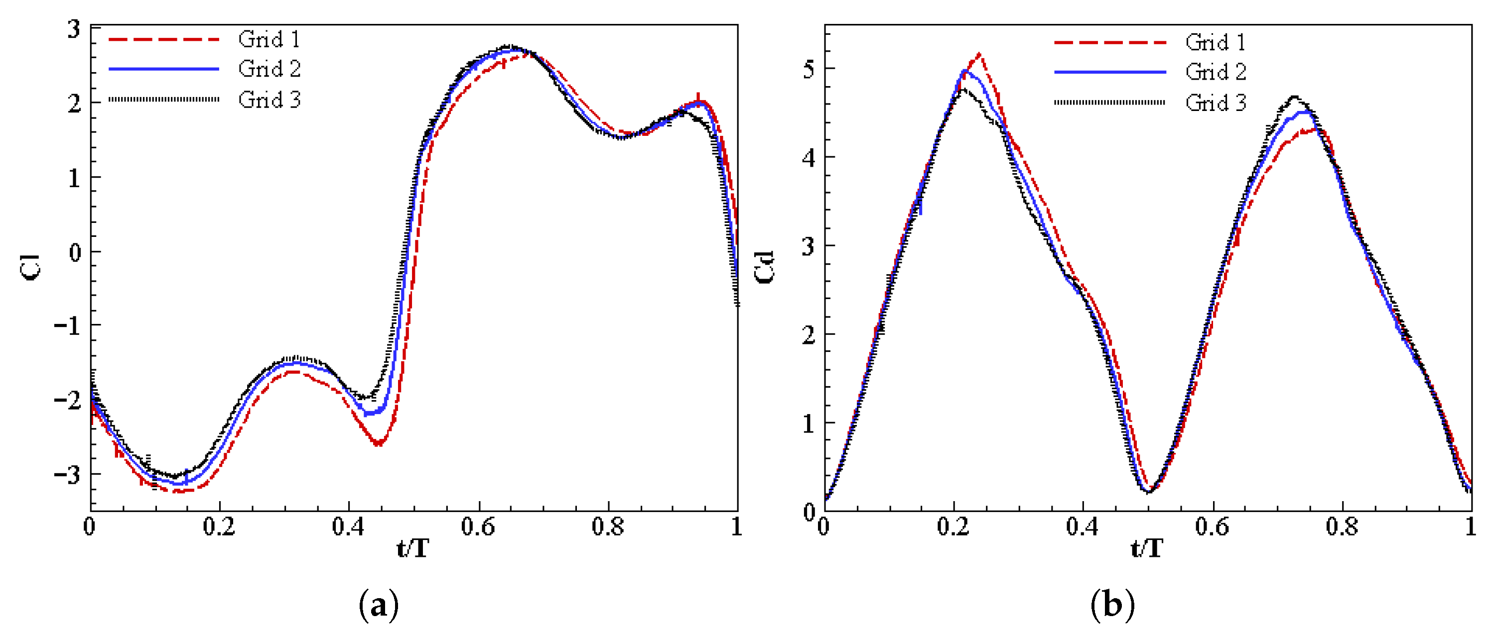
To verify the numerical accuracy of the LES turbulence method for the complex heave-pitch motion, a grid independence study was conducted at three different grid densities. As shown in

Table 1. Dynamic grid independent test with the results of $C{l}_{rms}$ and $C{d}_{avg}$ for numerical stability.

Name	Total Grids	${\mathit{Cl}}_{\mathit{rms}}$	Change (%)	${\mathit{Cd}}_{\mathit{avg}}$	Change (%)	Max. ${\mathit{y}}^{+}$
Grid 1	1,629,273	2.03	-	3.00	-	2.45
Grid 2	2,168,949	2.06	1.48%	3.02	0.33%	1.15
Grid 3	3,452,780	2.07	0.48%	3.02	0.00%	1.02

, the transition from Grid 1 to Grid 2 results in 0.33% and 1.48% changes in $C{d}_{avg}$ and $C{l}_{rms}$, respectively. When increasing the grid density to Grid 3 (3.45 million cells), no variation in the average drag coefficient and a very low 0.48% variation in the $C{l}_{rms}$ are observed, indicating that the solution is essentially grid-independent. This is also visually confirmed in Figure 3a,b, where the instantaneous $Cl$ and $Cd$ coefficient profiles over a normalized cycle ($t/T$) show that Grid 1 in the first half of the cycle from t/T = 0.05 to 0.65 shows underpredicted $Cl$ and also coasts larger $Cd$ from t/T = 0.2 to 0.4, with a peak value of 5.3 at t/T = 2.1. On the other hand, Grids 1 and 2 show nearly identical agreement in both $Cl$ and $Cd$. Moreover, the maximum value for $y^{+}$ was reduced from 2.45 on Grid 1 to 1.15 on Grid 2, thereby fulfilling the requirements of $y^{+}$ in LES to resolve boundary-layer turbulence without excessive damping. Although Grid 3 provides the highest theoretical accuracy, the incremental benefits are negligible (less than 0.5%), while the increased numerical costs are high compared to these benefits.

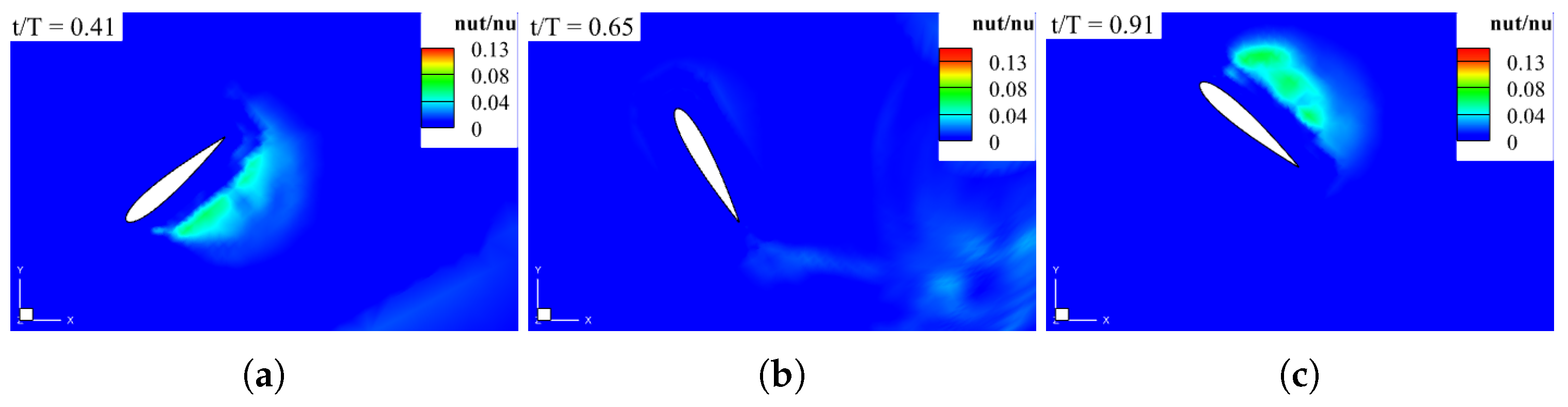
The effectiveness of the chosen grid (Grid 2) in resolving the small-scale vortical structure expected at $Re=5\times {10}^5$ was also tested by the ratio of the sub-grid scale eddy viscosity to the molecular viscosity (${\nu }_t/\nu$). As shown in Figure 4, the viscosity ratio is very low throughout the entire flow domain, not exceeding 0.13 even in the most turbulent instances of the vortex shedding process. However, the viscosity ratio is zero on the airfoil surface, which verifies that the flow within the viscous sub-layer is resolved rather than modeled. Based on the criteria given by Pope [20], this viscosity ratio confirms that the chosen grid is sufficiently fine to directly resolve the energy-containing range of the turbulent spectrum. While a finer grid will, in theory, improve this ratio even further, the minimal difference in aerodynamic coefficients between Grid 2 and Grid 3 verifies that this level of calculation is sufficient for the physics of this Reynolds number, and a finer grid will only provide unnecessary computational costs. Therefore, Grid 2 was determined to be the optimal mesh for all subsequent simulations, given its trade-off between accuracy and computational cost.

3.4. Validation of the Heave–Pitch Motions

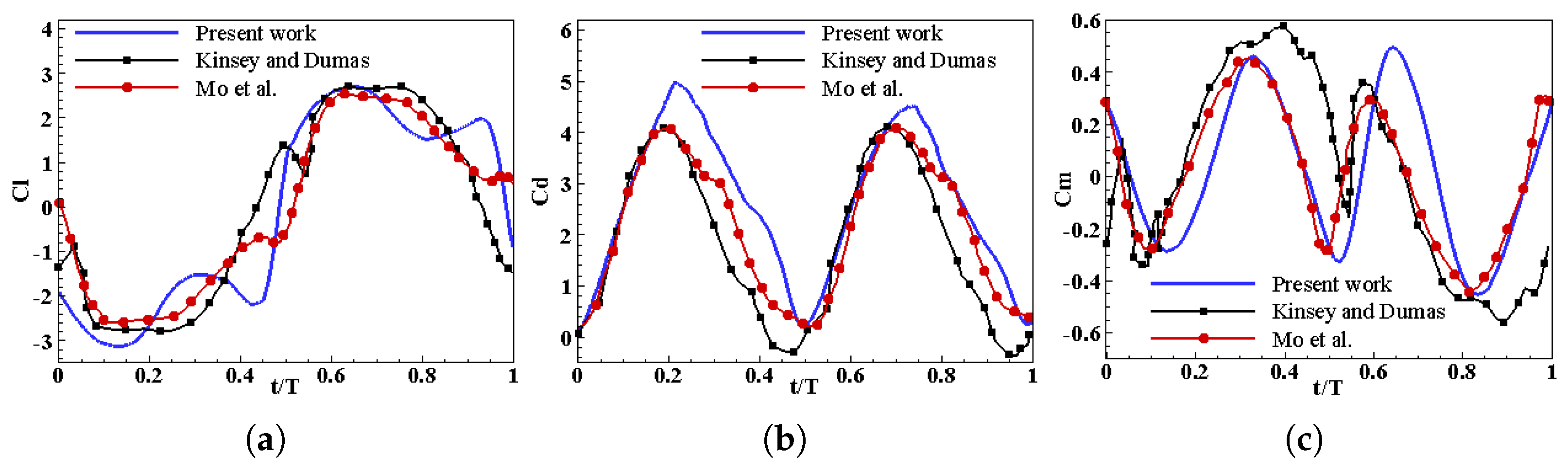
To ensure numerical accuracy, the present computational model is first validated against available benchmarks at $Re=5\times {10}^5$. As shown in Figure 5, the results are compared with the Ansys Fluent 13 (URANS-SA)-based solution of Kinsey and Dumas [29] and the OpenFOAM-based solution of Mo et al. [2]. As shown in the figures, the current high-fidelity LES-based simulation demonstrates excellent temporal synchronization, capturing the periodic nature of the lift, drag, and moment aerodynamic coefficients. Although RANS-based solutions yield smooth curves due to the eddy-viscosity model, LES simulations resolve with transient vortex dynamics, resulting in a peak drag coefficient of 5.0, as seen in Figure 5b, compared to the reference value of 4.0. Similarly, in Figure 5a, the peak lift force $C_l$ = 2.8 at $t/T=0.65$ matches well. The $C_m$ in Figure 5c is referenced to the $c/3$ point, showing the numerical results have accurately captured the periodic oscillations in the results, as well as the specific peaks in the results at $t/T=0.35$ and $t/T=0.65$, which are synchronized with the primary and secondary leading edge vortex shedding events in the lift and drag results. The matching results for the three aerodynamic coefficients $C_l$, $C_d$, and $C_m$ have therefore confirmed that the numerical framework is reliable for analyzing unsteady flow control mechanisms. However, the LES simulation captures higher fluctuations during stroke reversal at $t/T=0.2$ and 0.8. These discrepancies are expected because the LES simulation resolves the Leading Edge Vortex (LEV) dynamics at higher resolution, whereas the URANS formulation typically damps the sub-grid-scale dynamics.

3.5. Plasma Implementation Method

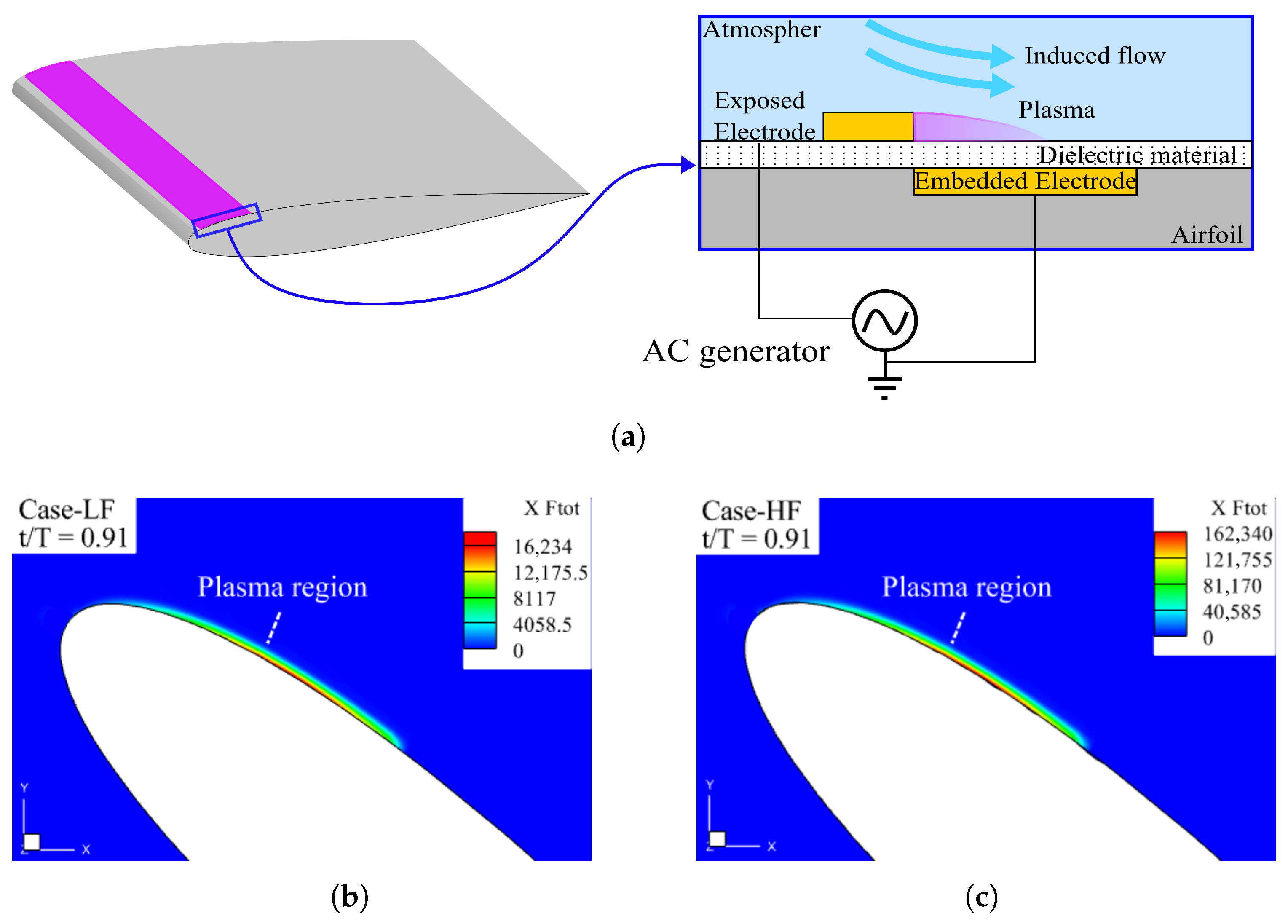
To mitigate the dynamic stall and enhance aerodynamic performance during the complex heave–pitch motions of the NACA 0015 airfoil, a DBD plasma actuator is installed at the leading edge. The plasma model is based on a phenomenological model, followed by the experimental and numerical setup by Singh et al. [26]. The body force $\mathbf{F}$ due to the plasma actuator is added as a source term to the momentum equation as seen in Equation (2); see Figure 6a. now the body force is split into its streamwise ($f_x$) and wall-normal ($f_y$) components, which are modeled with Gaussian decay functions to strictly localize the force in a thin region near the leading-edge surface, as shown in Equations (14)–(16) and Figure 6a below.

$$F=\left(f_x\right)\widehat{i}+\left(f_y\right)\widehat{j}$$

(14)

$$f_x=F_{x0}{\varphi }_0^{4}exp\left[-{\left({\displaystyle \frac{(-x-x_0)-(y-y_0)}{y}}\right)}^2-{\beta }_x{(y-y_0)}^2\right]$$

(15)

$$f_y=F_{y0}{\varphi }_0^{4}exp\left[-{\left({\displaystyle \frac{-x-x_0}{y}}\right)}^2-{\beta }_y{(y-y_0)}^2\right]$$

(16)

where F is the body force, $F_{x0}$ = $1.04\times {10}^{-5}$ and $F_{y0}$ = $-6.65\times {10}^{-5}$ are force constants, ${\varphi }_0$ denotes the voltage (in volts), which serves as the control parameter for the voltage magnitude, and is configured at 7000 volts. ${\beta }_x$ = $8\times {10}^{15}$, ${\beta }_y$ = ${10}^7$ are the decay constants, x is the center point between the exposed electrode and embedded electrode, and $y_0$ is the height of the dielectric surface.

The wing employed in this study undergoes changes in motion at different times, requiring the plasma position to adjust accordingly, as seen in Figure 6b,c. The parameter y in the equation plays a key role in this process. Based on the reference and the work of Moran [30], the NACA airfoil used in this work can be determined through a fourth-order equation to derive the wing shape, as expressed in Equation (17).

$$y=5ct\left[0.2969\sqrt{{\displaystyle \frac{x}{c}}}-0.1260\left({\displaystyle \frac{x}{c}}\right)-0.3516{\left({\displaystyle \frac{x}{c}}\right)}^2+0.2843{\left({\displaystyle \frac{x}{c}}\right)}^3-0.1015{\left({\displaystyle \frac{x}{c}}\right)}^4\right]$$

(17)

where y is the surface of the NACA 0015 airfoil, c is the chord length, and t = 0.036 m is the maximum thickness as a fraction of the chord.

To provide physical context to these dimensional values, the control authority is quantified via the momentum coefficient ($C_{\mu }$), as seen in Equation (18); this parameter scales the integrated plasma force against the freestream dynamic pressure ($q={\displaystyle \frac{1}{2}}\rho U_{\infty }^2$) [31], where ($U_{\infty }=2$ m/s). This provides a clear comparison between the actuator’s momentum injection and the inertial forces of the heave–pitch motion:

$$C_{\mu }={\displaystyle \frac{{\int }_V{f}_{x}dV}{\frac{1}{2}\rho U_{\infty }^2·c^2}}$$

(18)

where $C_{\mu }$ is the non-dimensional momentum coefficient, and V is the volume of the plasma discharge region where the body force is active.

The actuator schematic is shown in Figure 6a, and the AC-DBD technique induces a wall-parallel flow, designed to re-energize the boundary layer during complex heave–pitch motion [32]. The spatial distribution of the force is also presented for two cases at $t/T=0.91$ for demonstration purposes. Figure 6b shows the results for Case-LF, where the peak $f_x$ is 16,334 N/m³ while the $C_{\mu }$ is $0.050$. Figure 6c shows the results for the high-authority regime (Case-HF), where the force is tenfold higher, 163,340 N/m³, while $C_{\mu }$ is $0.508$. Additionally, the impact of the force is also shown as the rise in the induced pressure, $\Delta p_{plasma}=\int f_{x}dx$, for Case-HF, where the induced pressure reaches about 3267 Pa, while the freestream dynamic pressure $q_{\infty }={\displaystyle \frac{1}{2}}\rho U_{\infty }^2=2.45$ Pa, for $U_{\infty }=2$ m/s, indicating that the high-intensity direct drive configuration is strategically set for the imposition of the required local pressure gradient for the suppression of the large-scale dynamic stall vortex. When including the effect of $C_{\mu }$ non-dimensional based on the observed aerodynamic recovery, the aerodynamic enhancements are detailed in

Table 2. Aerodynamic performance analysis of baseline and plasma-based cases.

Parameters	Baseline	Case-LF	Improvement (%)	Case-HF	Improvement (%)
Peak $f_x$ (N/m3)	0	16,334	-	163,340	-
$C_{\mu }$	0	0.050	-	0.508	-
$C{l}_{rms}$	2.06	2.09	1.46	2.30	11.65
$C{d}_{avg}$	3.02	2.58	14.57	2.42	19.87
$C{l}_{rms}/C{d}_{avg}$	0.68	0.81	19.11	0.95	39.8

.

$C_{\mu }=0.508$ in the high-authority case is artificially elevated above the typical values observed in high-speed flight applications [31]. This is a mathematical consequence of the low freestream velocity, which is necessary to achieve the target Reynolds number of $5\times {10}^5$ for the given chord length. This artificially high coefficient is a mathematical artifact arising from the fact that the momentum coefficient is inversely proportional to the square of the freestream velocity (Equation (18)), and the non-dimensional forcing term appears artificially high even at the moderate strength of the body force. Phenomenologically, the high-momentum coefficient is necessary to access the high-authority limit and to explore the asymptotic limit of control authority. By over-powering the separation bubble, we can distinguish the various flow phenomena responsible for the flow transition from the stalled to the attached state. Although we recognize the need for optimal design to minimize energy expenditure for the application, in addition to enhancing aerodynamic performance, the goal of this work is to map the actuator’s maximum physical impact on the turbulent flow field.

4. Results and Discussion

In the previous sections, the computational environment was verified for the heave–pitch motion of NACA 0015, and after that, the plasma configurations at the leading edge of the airfoil were also verified; it remains attached at any position of the dynamic motion. Furthering these discussions, this section presents flow visualizations of an aerodynamic performance analysis for the heave–pitch motion of the airfoil. We compare the results for the cases with and without plasma actuation—baseline, without plasma; Case-LF, with a lower amount of plasma force; and Case-HF, with a larger amount of plasma force—at critical phases of the cycle (separation point at t/T = 0.41, peak Cl value at t/T = 0.65 and reattachment points at t/T = 0.91).

4.1. Aerodynamic Force Analysis

The unsteady aerodynamic behavior of the NACA 0015 airfoil during a full oscillation cycle is illustrated in Figure 7a,b, which shows variations in force production across three test cases. The quantification analysis of performance metrics is presented in Table 2. As seen in Figure 7a, the lift coefficient ($Cl$) of the blue solid line (Baseline) shows a local breakdown between $t/T=0.35$ and $0.45$, reaching a minimum of about $-2.02$ at $t/T=0.41$. Although the green line with triangle markers (Case-LF) closely follows the baseline trend, the black line with diamond markers (Case-HF) strongly mitigates this lift coefficient breakdown, maintaining a high value of about $-1.01$ at $t/T=0.41$. During this downstroke phase, the suction side becomes effective on the lower surface of the airfoil; the divergence in Case-HF indicates that the actuation effectively alters the flow topology on the lower surface, helping to avoid the strongest suction loss observed in the baseline case. The first two cases have a maximum lift of $Cl=2.75$ at $t/T=0.65$, and for the Case-HF, $Cl=2.8$ at the same point, which indicates the maximum impact of the dynamic stall vortex (DSV) on the upper surface during the upstroke phase. The drag coefficient ($Cd$) in Figure 7b also further emphasizes the effectiveness of the control strategy, where the black line (Case-HF) indicates a significantly lower peak value at $t/T=0.49$ compared to the baseline, which contributes to a $39.8\%$ enhancement in the overall $C{l}_{rms}/C{d}_{avg}$ ratio (Table 2). To understand these surface-specific phenomena, three key points have been selected for flow visualization: $t/T=0.41$ (suppression of the lower surface separation), $t/T=0.65$ (peak $Cl$ on the upper surface), and $t/T=0.91$ (the flow reattachment region) points in the following sections.

4.2. Spatiotemporal Flow Field Analysis

4.2.1. Velocity Contours Overlaid with Streamlines and Quantitative Assessment

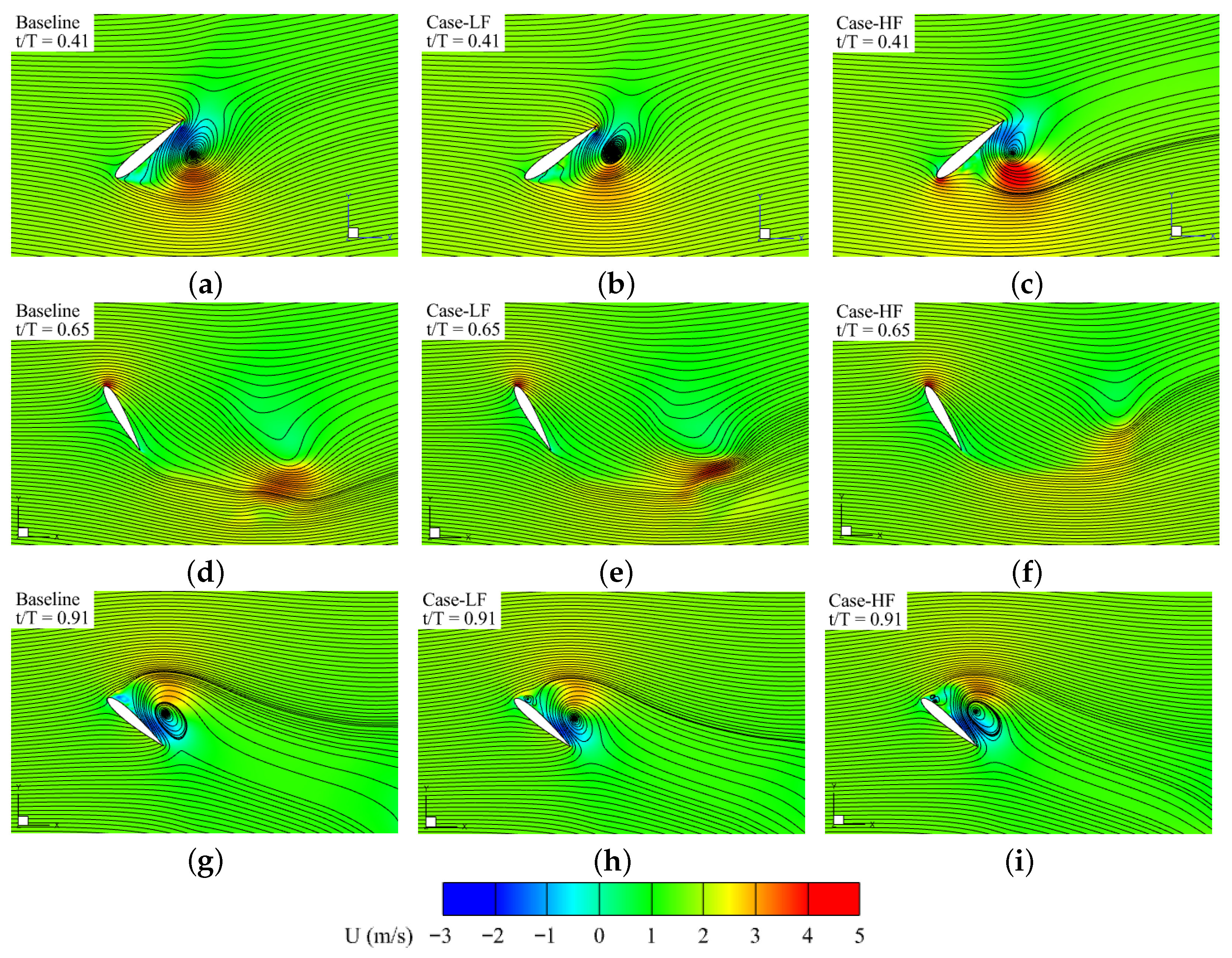
The velocity contours with the streamline are shown in Figure 8 indicating the flow topology at three critical points (flow onset, peak $Cl$, and reattachment points) in the three cases (baseline, Case-LF, and Case-HF). The increased plasma force in Case-HF fundamentally governs the dynamic stall life cycle, imposing a structural order on the phenomenon that the baseline and low-force Case-LF configurations lack. At the onset of stalling at $t/T=0.41$, both configurations exhibit the initiation of flow separation near the leading edge of the airfoil. However, in Case-HF, the developing vortex is fixed much closer to the upper surface of the airfoil, maintaining a coherent velocity core of magnitude exceeding $U=3$. As the life cycle progresses towards the maximum lift phase at $t/T=0.65$, both the baseline (Figure 8d) and Case-LF (Figure 8e) configurations exhibit massive vertical wake expansion and disordered high-velocity bumps, indicating a total breakdown of the shear layer. By contrast, the enhanced force of Case-HF (Figure 8f) converts these fragmented structures into a continuous, high-energy stream, preventing the widespread dispersal of the wake. This regularization of the dynamic stalled life cycle results in a remarkable recovery at $t/T=0.91$, where Case-HF (Figure 8i) exhibits a strikingly compact and flattened vortex core, while the other configurations remain obstructed by high-altitude re-circulation bubbles that hinder the return of the freestream.

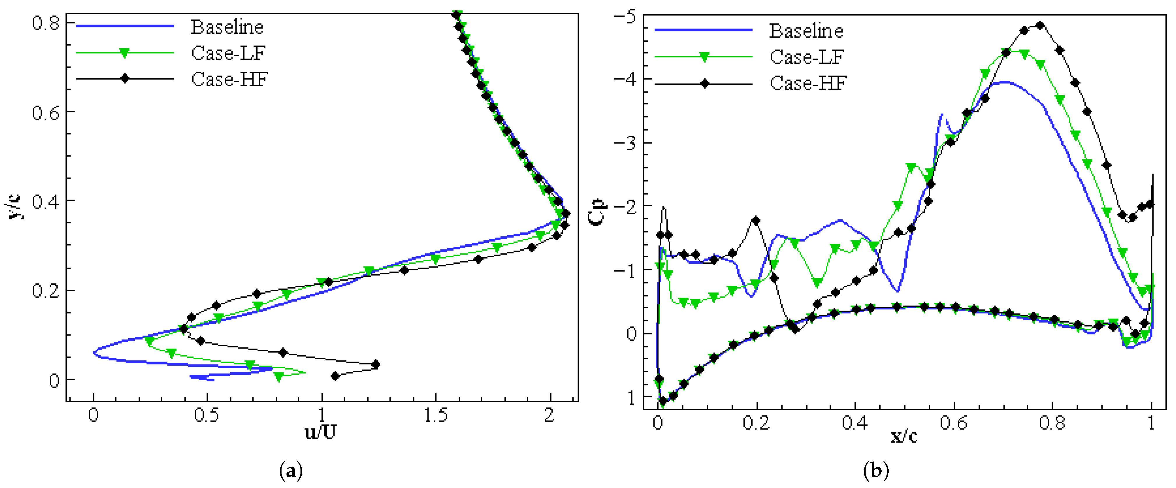
Figure 9 shows the quantitative results of the plasma’s effect on the flow at the specific reattachment point at $t/T=0.91$. The velocity profile shown in Figure 9a includes the extraction location $x/c=0.18$ from the top surface and immediately after the plasma position ends (the plane slice is taken from z = 0 (mid of the span)), and this velocity profile shows a significant level of momentum injected into the inner boundary layer, with a velocity nearly twice that of the baseline flow. This re-energizes the flow so that it can re-engage back towards the surface, and an effect is visually evident through the flattened velocity streams provided in Figure 8i. This resulted in the sharp recovery of the suction peak in the $Cp$ distribution shown in Figure 9b, where the baseline and Case-LF are still in the flat pressure state associated with the deep stall condition. By using the increased force required to counteract the high velocity of the velocity field, the actuator can shorten the stall period, transitioning the flow into an efficient high-lift state, whereas the lower force associated with Case-LF has no appreciable effect on aerodynamics.

4.2.2. Spatiotemporal Evolution of the Pressure Coefficient

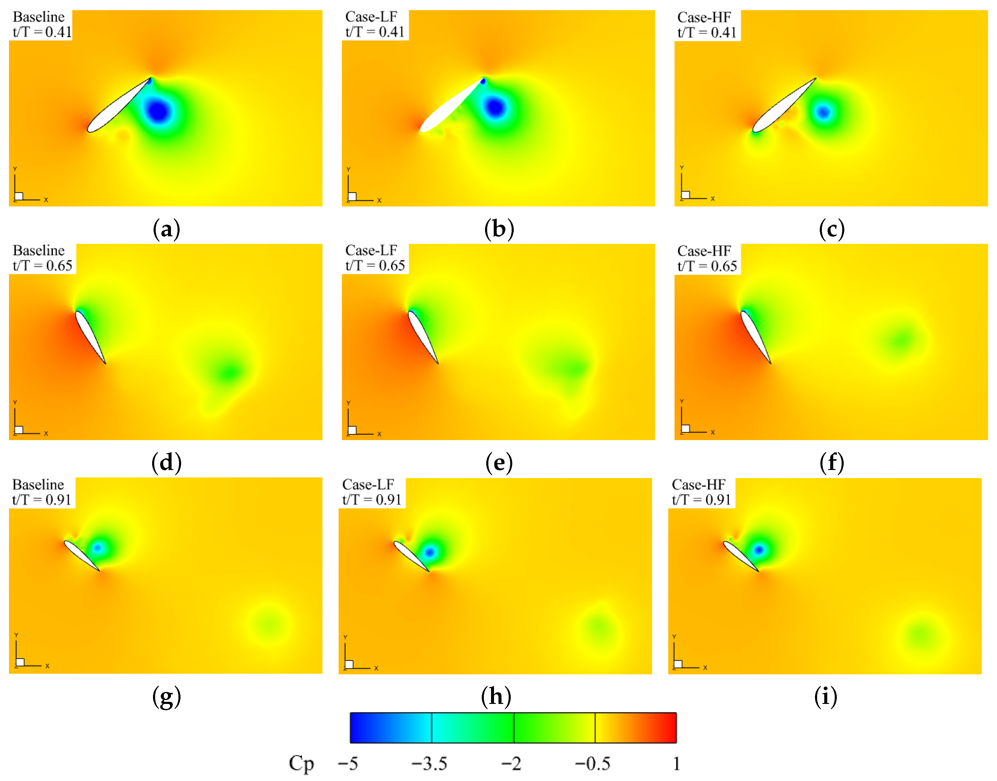
The pressure coefficient field is shown in Figure 10. It is evident that the fundamental change introduced by high-force plasma actuation is the reconfiguration of aerodynamic loading through the stabilization of the leading-edge suction at the onset of ($t/T=0.41$) (see the lower pressure region on the lower side of the leading edge in Figure 10c), while the baseline shown in Figure 10a and Case-LF, shown in Figure 10b, present a diffused and migrated low-pressure core in their configuration, while Case-HF’s configuration, shown in Figure 10c, presents a focused suction footprint with local $C_p$ values reaching a minimum of −8. Considering the freestream dynamic pressure of 2.45 Pa, the strong suction effect indicates a robust localized pressure drop. At the start of the downstroke, the lift coefficient is still developing; therefore, a focused low-pressure core is beneficial. During maximum lift development ($t/T=0.65$), the baseline was as shown in Figure 10d, and Case-LF was as shown in Figure 10e, presenting a dispersed pressure field, while Case-HF, shown in Figure 10f, presents a focused low-pressure core directly supporting the peak $Cl$ of 2.8. At the reattachment point $t/T=0.91$, the dominance of the high-force controls is again most apparent, with uncontrollable and low-force configurations impeded by the lingering presence of high-altitude low-pressure spots. In Case-LF, shown in Figure 10h, the rapid convergence and low-pressure bubbles can be observed, while in Case-HF, shown in Figure 10i, the swift formation of a pressure field is visible. This, in turn, causes the swift re-establishment of a sharp suction bulb ($Cp=-2$) at the leading edge, effectively shortening the trend of the deep stall and allowing the flow to re-engage with the surface much more aggressively than in the stagnant response of the low-force configuration and the baseline.

4.2.3. Vorticity Dynamics and Flow Structure

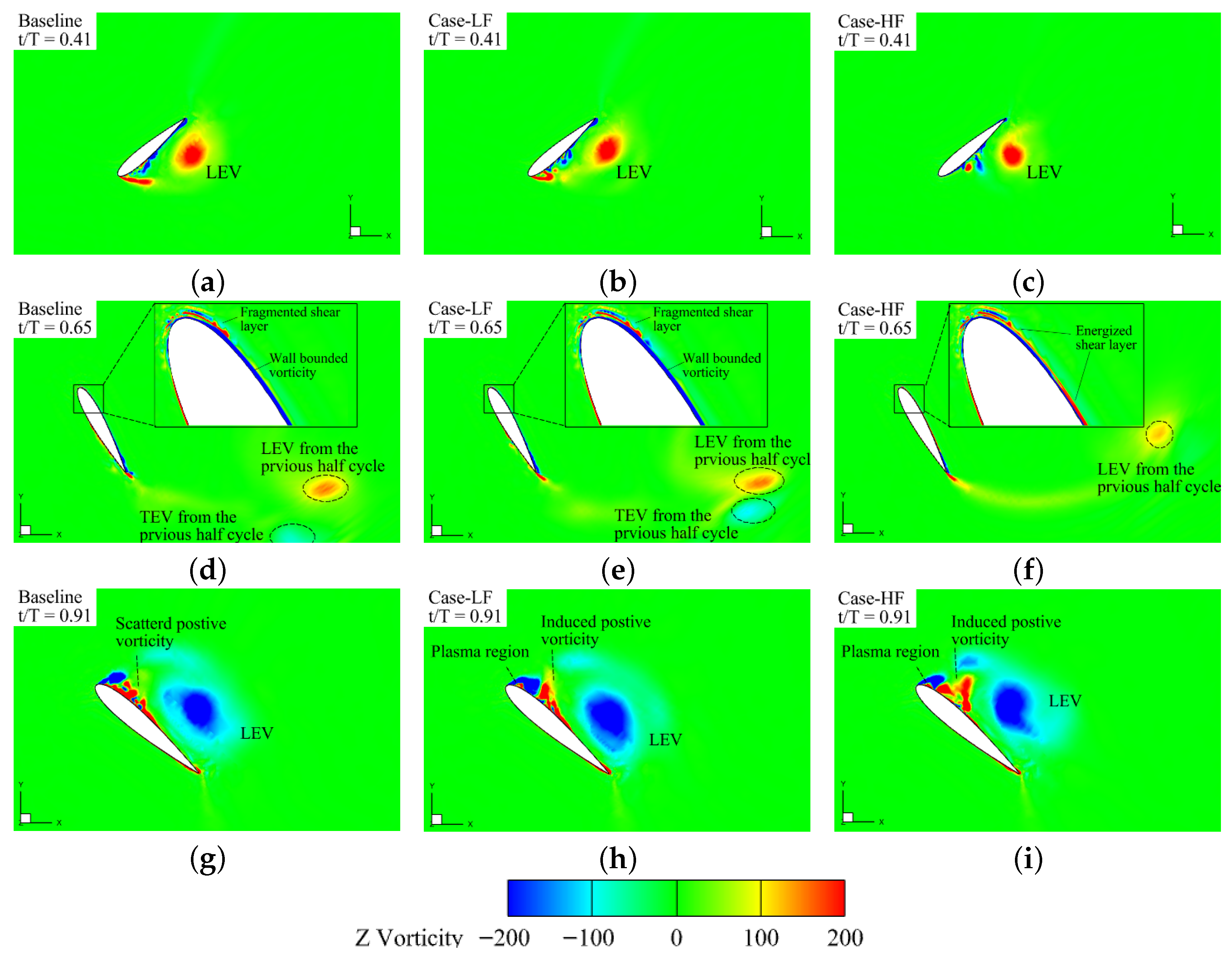
A detailed assessment of the vorticity distribution is shown in Figure 11, which illustrates how plasma actuation at high forces reconfigures the boundary-layer physics to delay stalling and improve recovery. For $t/T=0.41$ in the baseline case in Figure 11a and Case-LF, shown in Figure 11b, a diffuse LEV begins to detach. In contrast, in Case-HF (Figure 11c), the strongest plasma forces created a well-defined and potent LEV core closely associated with the upper surface. The major difference between the two cases is evident in the magnified view of the vortices at $t/T=0.65$. In the baseline (Figure 11d) and Case-LF (Figure 11e), the fragmented nature of the shear layers is apparent, with small-scale and highly irregular vortical structures. In stark contrast, in Case-HF (Figure 11f), the energized nature of the shear layer, with plasma forces eliminating fragmented instabilities, results in a thinner and stable vorticity distribution. This additional energy injection can also be seen in the remnants of the LEV from the previous half-cycle, which, in the higher-force cases, are more compact in the reattachment phase at $t/T=0.91$. The baseline (Figure 11g) struggles with scattered positive vorticity, hindering the flow, whereas Case-HF, shown in Figure 11i, uses the plasma regions to good effect to reenergize the flow with strong positive vorticity, pinning the flow to the surface. This ironing-out of the stalled legacy results in the rapid reformation of the boundary layer and the sharp pressure-suction peaks observed in previous figures.

4.2.4. Three-Dimensional Vortex and Coherence Analysis

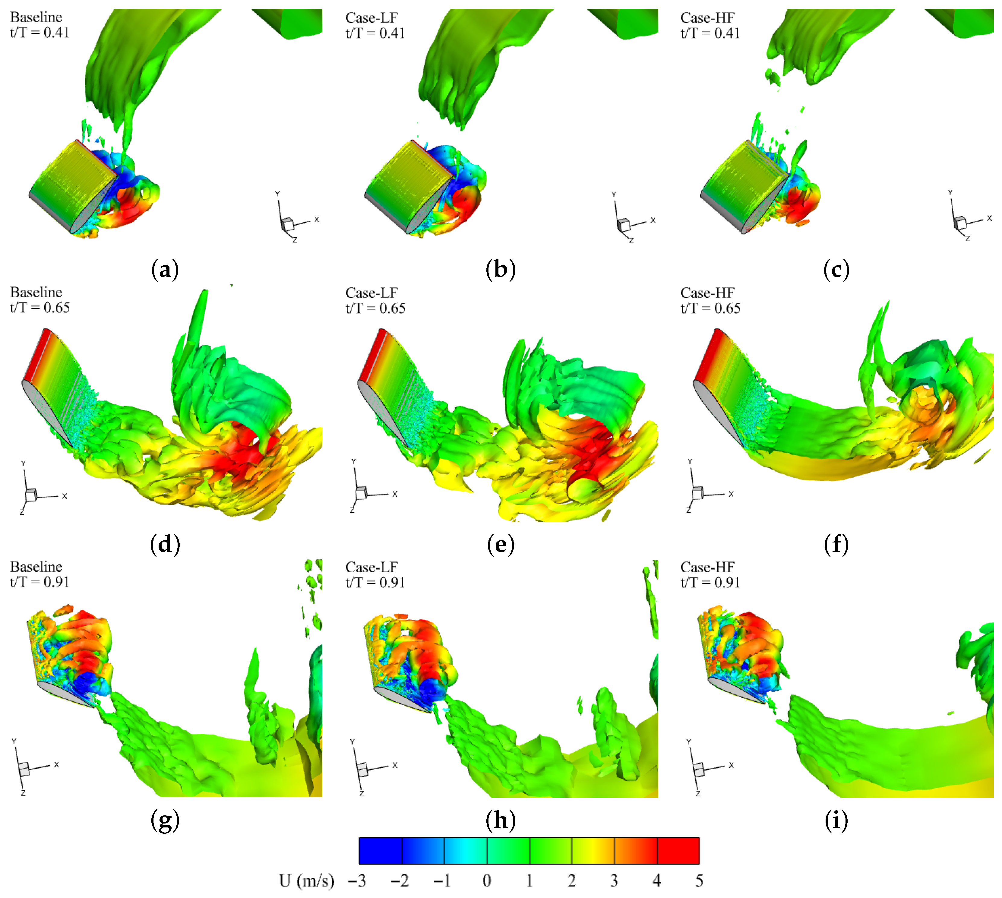
The development of three-dimensional flow structures, visualized using the Q-criterion [33] in Figure 12, provides a definitive explanation for the gains in macroscopic aerodynamic performance observed in the pressure field in Figure 10, and for the boundary-layer recovery observed in Figure 11. As the stall is initiated at $t/T=0.41$, the high-force actuation of Case-HF (Figure 12c) creates a more coherent and high-velocity LEV compared to the diffuse and low-momentum flow of the baseline (Figure 12a) and Case-LF (Figure 12b). As the cycle progresses to the deeper stall condition at $t/T=0.65$, the baseline (Figure 12d) and Case-LF (Figure 12e) show a more locally fragmented, large resurculation of vortex to the airfoil and disordered wakes, which correspond to pressure scattering, as seen in Figure 10d,e. Case-HF (Figure 12f) retains a regularized and elongated LEV. This structural regime suppresses the unorganized energy dissipation associated with uncontrollable stall, thereby enhancing reattachment. More importantly, in the reattachment phase ($t/T=0.91$), Case-HF (Figure 12i) displays a swift confluence of flows to a compact structure with high near-wall momentum ($U\approx 4$), precisely matching the sharp recovery in suction ($Cp=-5$) shown in Figure 9b and the energized velocity profiles in Figure 9a. These 3D structures ultimately reveal that the increased plasma forces resolved unorganized shedding to a streamlined, high-lift state, which cannot be sustained by the low-force case of Case-LF.

4.3. Aerodynamic Performance Enhancement

Table 2 shows an aerodynamic performance analysis of the uncontrolled baseline and the high-force actuation cases. A comparison shows that although both plasma cases improve Cl increments and Cd mitigation, Case-LF offers only a slight improvement in Cl, whereas Case-HF achieves a large $11.65\%$ increase in $C{l}_{rms}$, mainly through LEV dynamics during high-amplitude heave–pitch motions. More importantly, the plasma-induced momentum addition greatly reduces the drag cost of the aggressive flapping motion; $C{d}_{avg}$ of the baseline decreases from $3.02$ to $2.42$ in Case-HF, indicating a $19.87\%$ relative enhancement in aerodynamic performance. The coupling of improved lift and drag performance is best captured by the aerodynamic efficiency ratio ($C{l}_{rms}/C{d}_{avg}$), which increases from a baseline value of $0.68$ to $0.95$. This is a $39.8\%$ relative enhancement in the efficiency index, indicating that high-force plasma actuation not only adds momentum locally but also radically alters the wake structure, promoting thrust production and structural loading. These results clearly indicate that active flow control can enhance the flight effectiveness of flapping wings at $Re=5\times {10}^5$ across different aerodynamic system applications.

5. Conclusions

The integration of active flow control with the complex motion of an airfoil presents one of the most promising research frontiers for aerospace applications, offering a versatile, high-response mechanism for addressing unsteady flight maneuvers. Although previous research has focused on pure pitching motion with 2D airfoil shapes, these do not really capture the real-world problem. The present study employed the high-fidelity LES method to examine the combined effect of the heave–pitch motion of a 3D NACA 0015 airfoil with plasma-based AFC to control the dynamic stall and improve the aerodynamic performance at $Re=5\times {10}^5$. The simulation results indicate that high-force plasma actuation offers a transformative mechanism for regularizing 3D dynamic stall motion. The aggressive injection of momentum into the near-wall region effectively reduces uncontrolled, fragmented, and high-velocity vortical structures. Such structural discipline ensures that a compact, high-intensity wall-bound leading-edge vortex forms and remains attached to the suction surface for significantly longer periods than the baseline and Case-LF cases.

This restriction in wake growth prevented the massive lift-off of vortical structures, and a rapid re-engagement of the flow is forced during the critical reattachment phase at $t/T=0.91$. The restoration of a sharp leading-edge suction peak, in which local pressure values reach the minimum scale value of $-5$, is the physical mechanism behind the significant aerodynamic benefits observed throughout the complex heave–pitch cycle. In detail, the transition from low-force to higher-force actuation yields a dramatic improvement in aerodynamic efficiency, with the $C{l}_{rms}/C{d}_{avg}$ ratio increasing by 39.8% relative to the baseline. There is a critical force threshold that must be exceeded to transition the flow topology from a disordered deep-stall configuration to a controlled, high-lift configuration that maximizes overall aerodynamic performance and lifting efficiency.

Although this 3D LES framework provides a significant understanding of fundamental vortical phenomena, it serves as a bridge to several potential future research trends. Specifically, the current use of a phenomenological plasma model, along with validation discrepancies, suggests that future simulations could include more complex electro-hydrodynamic effects. Ultimately, future extensions of this research will include simulations over a range of different Reynolds numbers. There is also significant potential to explore the experimental use of plasma actuators for multi-degree-of-freedom airfoil motion, enabling the dynamic optimization of actuator output to maximize net energy efficiency in practical aero-structural applications.

References

1. Shyy, W.; Berg, M.; Ljungqvist, D. Flapping and flexible wings for biological and micro air vehicles. Prog. Aerosp. Sci. 1999, 35, 455–505. [Google Scholar] [CrossRef] [Scilit]
2. Mo, W.; He, G.; Wang, J.; Zhang, Z.; Gao, Y.; Zhang, W.; Sun, L.; Ghassemi, H. Hydrodynamic analysis of three oscillating hydrofoils with wing-in-ground effect on power extraction performance. Ocean Eng. 2022, 246, 110642. [Google Scholar] [CrossRef] [Scilit]
3. Ham, N.D.; Garelick, M.S. Dynamic stall considerations in helicopter rotors. J. Am. Helicopter Soc. 1968, 13, 49–55. [Google Scholar] [CrossRef] [Scilit]
4. Young, J.; Lai, J.C.; Platzer, M.F. A review of progress and challenges in flapping foil power generation. Prog. Aerosp. Sci. 2014, 67, 2–28. [Google Scholar] [CrossRef] [Scilit]
5. Kinsey, T.; Dumas, G. Optimal operating parameters for an oscillating foil turbine at Reynolds number 500,000. AIAA J. 2014, 52, 1885–1895. [Google Scholar] [CrossRef] [Scilit]
6. He, G.; Mo, W.; Gao, Y.; Zhang, Z.; Wang, J.; Wang, W.; Liu, P.; Ghassemi, H. Modification of effective angle of attack on hydrofoil power extraction. Ocean Eng. 2021, 240, 109919. [Google Scholar] [CrossRef] [Scilit]
7. Tayebi, A.; Torabi, F. Flow control techniques to improve the aerodynamic performance of Darrieus vertical axis wind turbines: A critical review. J. Wind. Eng. Ind. Aerodyn. 2024, 252, 105820. [Google Scholar] [CrossRef] [Scilit]
8. Tousi, N.; Coma, M.; Bergadà, J.; Pons-Prats, J.; Mellibovsky, F.; Bugeda, G. Active flow control optimisation on SD7003 airfoil at pre and post-stall angles of attack using synthetic jets. Appl. Math. Model. 2021, 98, 435–464. [Google Scholar] [CrossRef] [Scilit]
9. Sato, M.; Nonomura, T.; Okada, K.; Asada, K.; Aono, H.; Yakeno, A.; Abe, Y.; Fujii, K. Mechanisms for laminar separated-flow control using dielectric-barrier-discharge plasma actuator at low Reynolds number. Phys. Fluids 2015, 27, 117101. [Google Scholar] [CrossRef] [Scilit]
10. Omidi, J. Advances and opportunities in wind energy harvesting using plasma actuators: A review. Clean Energy 2024, 8, 197–225. [Google Scholar] [CrossRef] [Scilit]
11. Kong, W.; Guo, K.; Li, Y. Study on the Active Control of the Dynamic Stall of Rotor Airfoils Based on Plasma Excitation. Aerospace 2024, 11, 474. [Google Scholar] [CrossRef] [Scilit]
12. Woo, G.T.; Glezer, A. Transitory control of dynamic stall on a pitching airfoil. In Proceedings of the Active Flow Control II: Papers Contributed to the Conference” Active Flow Control II 2010”, Berlin, Germany, 26–28 May 2010; Springer: Berlin/Heidelberg, Germany, 2010; pp. 3–18. [Google Scholar] [CrossRef] [Scilit]
13. Visbal, M.R. Control of dynamic stall on a pitching airfoil using high-frequency actuation. In Proceedings of the 53rd AIAA Aerospace Sciences Meeting, Kissimmee, FL, USA, 5–9 January 2015; AIAA: Reston, BA, USA, 2015; p. 1267. [Google Scholar] [CrossRef] [Scilit]
14. Xie, C.; Gao, N.; Meng, Y.; Wu, Y.; Yang, C. A review of bird-like flapping wing with high aspect ratio. Chin. J. Aeronaut. 2023, 36, 22–44. [Google Scholar] [CrossRef] [Scilit]
15. Post, M.L.; Corke, T.C. Separation control on high angle of attack airfoil using plasma actuators. AIAA J. 2004, 42, 2177–2184. [Google Scholar] [CrossRef] [Scilit]
16. Corke, T.C.; Enloe, C.L.; Wilkinson, S.P. Dielectric barrier discharge plasma actuators for flow control. Annu. Rev. Fluid Mech. 2010, 42, 505–529. [Google Scholar] [CrossRef] [Scilit]
17. Lee, T.; Gerontakos, P. Investigation of flow over an oscillating airfoil. J. Fluid Mech. 2004, 512, 313–341. [Google Scholar] [CrossRef] [Scilit]
18. Foias, C.; Manley, O.; Rosa, R.; Temam, R. Navier-Stokes Equations and Turbulence; Cambridge University Press: Cambridge, UK, 2001; Volume 83. [Google Scholar]
19. Sagaut, P. Large Eddy Simulation for Incompressible Flows: An Introduction; Springer Science & Business Media: Berlin/Heidelberg, Germany, 2005. [Google Scholar]
20. Pope, S.B. Turbulent flows. Meas. Sci. Technol. 2001, 12, 2020–2021. [Google Scholar] [CrossRef] [Scilit]
21. Weller, H.G.; Tabor, G.; Jasak, H.; Fureby, C. A tensorial approach to computational continuum mechanics using object-oriented techniques. Comput. Phys. 1998, 12, 620–631. [Google Scholar] [CrossRef] [Scilit]
22. Justin, S.; Jonathan, M. Deep learning closure models for large-eddy simulation of flows around bluff bodies. J. Fluid Mech. 2023, 966, A26. [Google Scholar] [CrossRef] [Scilit]
23. Kim, D.H.; Chang, J.W. Low-Reynolds-number effect on the aerodynamic characteristics of a pitching NACA0012 airfoil. Aerosp. Sci. Technol. 2014, 32, 162–168. [Google Scholar] [CrossRef] [Scilit]
24. OpenCFD Ltd. OpenFOAM User Guide; OpenCFD Ltd.: Berkshire, UK, 2016. [Google Scholar]
25. Souli, M.; Zolesio, J. Arbitrary Lagrangian–Eulerian and free surface methods in fluid mechanics. Comput. Methods Appl. Mech. Eng. 2001, 191, 451–466. [Google Scholar] [CrossRef] [Scilit]
26. Singh, K.P.; Roy, S. Force approximation for a plasma actuator operating in atmospheric air. J. Appl. Phys. 2008, 103, 013305. [Google Scholar] [CrossRef] [Scilit]
27. Mukherjee, S.; Roy, S. Enhancement of lift and drag characteristics of an oscillating airfoil in deep dynamic stall using plasma actuation. In Proceedings of the 50th AIAA Aerospace Sciences Meeting Including the New Horizons Forum and Aerospace Exposition, Nashville, TN, USA, 9–12 January 2012; AIAA: Reston, BA, USA, 2012; p. 702. [Google Scholar] [CrossRef] [Scilit]
28. Dolla, D.A.; Wang, C.C. Investigation of plasma actuator configurations for the dynamic heave-pitch motion of an airfoil through large eddy simulations. Phys. Fluids 2026, 38, 025135. [Google Scholar] [CrossRef] [Scilit]
29. Kinsey, T.; Dumas, G. Computational fluid dynamics analysis of a hydrokinetic turbine based on oscillating hydrofoils. J. Fluids Eng. 2012, 134, 021104. [Google Scholar] [CrossRef] [Scilit]
30. Moran, J. An Introduction to Theoretical and Computational Aerodynamics; Courier Corporation: Chelmsford, MA, USA, 2003. [Google Scholar]
31. Seifert, A.; Bachar, T.; Koss, D.; Shepshelovich, M.; Wygnanski, I. Oscillatory blowing: A tool to delay boundary-layer separation. AIAA J. 1993, 31, 2052–2060. [Google Scholar] [CrossRef] [Scilit]
32. Wang, C.C.; Dolla, D.A.; Wang, Y.C. Active Flow Control Analysis Over an Oscillating NACA 0012 Airfoil Using Sinusoidal Energy Deposition. Aerosp. Sci. Technol. 2026, 175, 111928. [Google Scholar] [CrossRef] [Scilit]
33. Chakraborty, P.; Balachandar, S.; Adrian, R.J. On the relationships between local vortex identification schemes. J. Fluid Mech. 2005, 535, 189–214. [Google Scholar] [CrossRef] [Scilit]
Figure 1. Heave–pitch motions of NACA 0015. (a) Schematic of airfoil motion along with flow field. (b) Sinusoidal motion demonstrations.
Actuators 15 00190 g001
Figure 2. Computational model. (a) Boundary condition. (b) Generated mesh profile.
Actuators 15 00190 g002
Figure 3. Grid independence study comparing three grid levels. (a) The time history of C l . (b) C d over one complete heave–pitch cycle.
Actuators 15 00190 g003
Figure 4. Instantaneous eddy viscosity ratio ( ν t / ν ) contours for the Grid 2 (Baseline case) at (a) t / T = 0.41 , (b) t / T = 0.65 , and (c) t / T = 0.91 . The peak levels of ( ν t / ν ) are all quite low (≈0.13), and those near the wall are vanishingly small, which is indicative of a well-resolved LES.
Actuators 15 00190 g004
Figure 5. Validation of instantaneous aerodynamic coefficients for a flapping airfoil at ( R e = 5 × 10 5 , f * = 0.14 , θ 0 = 75 , h 0 = c , x p / c = 1 / 3 ) [2,29]: (a) lift coefficient ( C l ); (b) drag coefficient ( C d ); (c) moment coefficient ( C m ).
Actuators 15 00190 g005
Figure 6. Analysis of the AC-DBD plasma actuator and the horizontal body force distribution after simulation. (a) Schematic of AC-DBD formation. (b) Case-LF. (c) Case-HF at t / T = 0.91 .
Actuators 15 00190 g006
Figure 7. Time history of aerodynamic force coefficients. (a) Cl variation over one motion cycle. (b) Cd.
Actuators 15 00190 g007
Figure 8. Velocity contours with streamlined flow visualization comparing the baseline (a,d,g), Case-LF (b,e,h), and Case-HF (c,f,i) at critical cycle phases.
Actuators 15 00190 g008
Figure 9. Boundary layer characteristics and surface loading during the reattachment phase ( t / T = 0.91 , A O A = 42 ). (a) Velocity profile at x / c = 0.18 ; (b) surface Cp distribution.
Actuators 15 00190 g009
Figure 10. Spatiotemporal static pressure coefficient for the baseline (a,d,g), Case-LF (b,e,h), and Case-HF (c,f,i) at critical cycle phases.
Actuators 15 00190 g010
Figure 11. Z-vorticity evolution for the baseline (a,d,g), Case-LF (b,e,h), and Case-HF (c,f,i) at the critical cycle phases. Insets at t / T = 0.65 provide a magnified view of the leading-edge shear layer stability.
Actuators 15 00190 g011
Figure 12. Iso-surfaces of Q-criterion colored by velocity magnitude (U) for baseline (a,d,g), Case-LF (b,e,h), and Case-HF (c,f,i), at the three critical phases of the cycle.
Actuators 15 00190 g012